Discrete Wigner functions and the phase space representation of quantum computers

Abstract

We show how to represent the state and the evolution of a quantum computer (or any system with an $N$–dimensional Hilbert space) in phase space. For this purpose we use a discrete version of the Wigner function which, for arbitrary $N$, is defined in a phase space grid of $2N\times 2N$ points. We compute such Wigner function for states which are relevant for quantum computation. Finally, we discuss properties of quantum algorithms in phase space and present the phase space representation of Grover’s quantum search algorithm.

2

Wigner functions [1] provide a simple representation of the quantum state of a continuous system in phase space. This is important when analyzing issues related with the classical limit of quantum mechanics [2]. In this letter we study a useful generalization of the Wigner function to systems with $N$–dimensional Hilbert spaces. We use this Wigner function to obtain, for the first time, a phase space representation of both the states and the temporal evolution of a quantum computer. What are the potential advantages of a phase space representation of a quantum computer? It is clear that quantum algorithms can be thought of as quantum maps operating in a finite state space and are therefore amenable to this representation. Whether it will be useful or not will depend on properties of the algorithm. Specifically, algorithms become interesting in the large $N$ limit (i.e. when operating on many qubits). For a quantum map this is the semiclassical limit where many new regularities arise in connection with its classical behaviour in phase space. Thus unraveling these regularities, when they exist, becomes an important issue which can be naturally accomplished in a phase space representation. Moreover, this phase space approach may allow one to establish contact between the vast literature on quantum maps (dealing with their construction, semiclassical properties, etc) and that of quantum algorithms providing hints to develop new algorithms. As a first application of these ideas we show how Grover’s search algorithm [3] can be represented in phase space and interpreted as a simple quantum map.

For a particle in $1$ dimension the Wigner function, [1]

$$W(q,p)=\int{d\lambda\over{2\pi\hbar}}e^{-i\lambda p/\hbar}\langle q-{\lambda\over 2}|\hat{\rho}|q+{\lambda\over 2}\rangle,.$$ (1)

has the following properties: (P1) $W(q,p)$ is real valued, (P2) The inner product between states $\rho_{1}$ and $\rho_{2}$ is $Tr(\rho_{1}\rho_{2})=2\pi\hbar\int dqdpW_{1}(q,p)W_{2}(q,p)$, (P3) The integral of $W(q,p)$ along a line in phase space, defined as $a_{1}q+a_{2}p=a_{3}$, is the probability density that a measurement of the observable $a_{1}\hat{Q}+a_{2}\hat{P}$ has $a_{3}$ as a result. These properties follow directly from the definition (1). However, their origin can be better understood by noticing that $W(q,p)$ is the expectation value of an operator $\hat{A}(q,p)$, known as ”phase space point operator”:

$$W(q,p)=Tr(\hat{\rho}\hat{A}(q,p)).$$ (2)

The operator $\hat{A}(q,p)$, that parametrically depends on $(q,p)$, is a symmetrized product of delta functions:

$$\hat{A}(q,p)=\int\!\!\int{d\lambda d\lambda^{\prime}\over{(2\pi\hbar)^{2}}}\ e^{i{\lambda\over\hbar}(\hat{Q}-q)-i{\lambda^{\prime}\over\hbar}(\hat{P}-p)}$$ (3)

Properties (P1-P3) follow directly from simple properties of $\hat{A}(q,p)$. In fact, reality of $W(q,p)$ is a consequence of the hermiticity of $\hat{A}(q,p)$. The inner product rule follows from the fact that $\hat{A}(q,p)$ are complete in the sense that $Tr(\hat{A}(q,p)\hat{A}(p^{\prime},q^{\prime}))=\delta(q-q^{\prime})\delta(p-p^{\prime})/2\pi\hbar$. Finally, property (P3) is a consequence of the fact that when integrating $\hat{A}(q,p)$ over a line in phase space one gets a projection operator: $\int dpdq\delta(a_{1}q+a_{2}p-a_{3})\hat{A}(q,p)=|a_{3}\rangle\langle a_{3}|$ where $|a_{3}\rangle$ is an eigenstate of the operator $a_{1}\hat{Q}+a_{2}\hat{P}$ with eigenvalue $a_{3}$. Notice that although the above definitions are given in terms of $\hat{P}$ and $\hat{Q}$, only unitary exponentials of such operators (i.e, finite phase space translations) are involved in (3).

To define Wigner functions for discrete systems various attempts can be found in the literature. Most notably, Wooters [4] proposes a definition that has the properties (P1–P3) only when $N$ is a prime number. His phase space is an $N\times N$ grid (if $N$ is prime) and a cartesian product of spaces corresponding to prime factors of $N$ in the general case. Rivas and Ozorio de Almeida [5] define translation and reflection operators relating to the geometry of chords and centers on the phase space torus. Bouzouina and De Bievre [6] give a more abstract derivation relating to geometric quantization. Our approach here follows closely Wooters ideas but combine them with the results in [5] to obtain a Wigner function with all the required properties (including the generalization of (P3)).

Given a basis of Hilbert space (for example, the computational basis of a quantum computer) $B_{x}=\{|n\rangle,n=0,..,N-1\}$ we can think of it as a discretized coordinate basis (with periodic boundary conditions). Its discrete Fourier transform $B_{p}=\{|k\rangle,k=0,..,N-1\}$, related to $B_{x}$ by $|k\rangle=\sum_{n}\exp(i2\pi nk/N)|n\rangle/\sqrt{N}$, can be considered as the corresponding momentum basis (with the same periodicity). For a system with an $N$ dimensional Hilbert space it is not possible to define hermitian position and momentum operators that generate infinitesimal displacements. As Schwinger has shown [7], this shortcoming is overcome by introducing unitary operators that generate finite displacements. The translation operator $\hat{U}$ generates cyclic shifts in the position basis, i.e. $\hat{U}^{m}|n\rangle=|n+m\rangle$. On the other hand, displacement operators in the momentum basis satisfy $\hat{V}^{m}|k\rangle=|k+m\rangle$ and are diagonal in the $B_{x}$ basis: $\hat{V}^{m}|n\rangle=\exp(i2\pi mn/N)|n\rangle$ (analogously, $\hat{U}$ is diagonal in the $B_{p}$ basis: $\hat{U}^{n}|k\rangle=\exp(-i2\pi kn/N)|k\rangle$). The commutation relations between $\hat{U}$ and $\hat{V}$ take the form $\hat{U}\hat{V}=\hat{V}\hat{U}\exp{(-2i\pi/N)}$ [7]. Using this it is easy to show that the operator $\hat{T}(m,k)=\hat{U}^{m}\hat{V}^{k}\exp(i\pi mk/N)$ is the discrete equivalent of the symmetrized displacement $\exp{{i\over\hbar}(q\hat{P}-p\hat{Q})}$ in the continuous case.

With these tools, it is natural to generalize (3) as

$$\hat{\cal A}(q,p)={1\over N^{2}}\sum_{m,k=0}^{N-1}\hat{T}(m,k)\exp{\{-i2\pi{(kq-mp)\over N}\}}.$$

However, one immediately sees that this definition has a serious problem: Thus, for real values of $(q,p)$ the operators defined in this way are not hermitian. This problem comes as no surprise since the use of an integer grid does not allow the half-points needed in (1). As previous works indicate [8], there is an obvious solution to this problem which simply consists of defining Wigner functions in an array of $2N\times 2N$ points (lying at half-integer values of $q,p$). This leads to the following definition of phase space point operators in the discrete case

$$\hat{A}(q,p)={1\over(2N)^{2}}\sum_{\lambda,\lambda^{\prime}=0}^{2N-1}\hat{T}(\lambda,\lambda^{\prime})\exp{\{-i2\pi{(\lambda^{\prime}q-\lambda p)\over 2N}\}}$$ (4)

where now $q,p$ are integers in the range $\{0,...,2N-1\}$

It is simple to show that these operators have all the desired properties and enable us to define the Wigner function exactly as in (2) (i.e., the discrete Wigner function is the expectation value of the discrete phase space point operator (4)). First, the operators $\hat{A}(q,p)$ are Hermitian. Second, they form a complete set. Therefore, one can always invert equation (2) and express $\hat{\rho}$ as a linear combination of $\hat{A}(q,p)$. In fact, the Wigner function are the coefficients of such expansion: i.e.

$$\hat{\rho}=N\sum_{p,q}^{2N-1}W(q,p)\hat{A}(q,p).$$ (5)

Using this, it is simple to show that the inner product between two states is obtained from the corresponding Wigner functions as: $Tr(\rho_{1}\rho_{2})=N\sum_{q,p}W_{1}(q,p)W_{2}(q,p)$. It is worth noticing that the number of phase space point operators is $4N^{2}$ but that there are only $N^{2}$ of them that are linearly independent. A basis set for such operators is formed by the ones corresponding to points with $0\leq q,p\leq N-1$, belonging to the first square subgrid of $N\times N$ points of the original $2N\times 2N$ lattice. Thus, the entire Wigner function is determined by the values it takes on this first square subgrid. In fact, one can show that $W(\sigma_{q}N+q,\sigma_{p}N+p)=(-1)^{\sigma_{q}p+\sigma_{p}q+N\sigma_{p}\sigma_{q}}W(q,p)$, an expression that relates the values of the Wigner function on the four different $N\times N$ subgrids.

Generalizing property (P3) to the discrete case is less trivial. Following Wooters [4], we can define a line $L$ in the phase space grid as the set of points $L(n_{1},n_{2},n_{3})=\{(q,p){\rm\ such\ that\ }n_{1}q+n_{2}p=n_{3}\}$ with $0\leq n_{i}\leq 2N-1$ (two lines are parallel if they are parametrized by the same integers $n_{1}$ and $n_{2}$ but differ in $n_{3}$). It is possible to show that the above Wigner function satisfies the following crucial property: When adding its value over all points belonging to a line $L(n_{1},n_{2},n_{3})$ one always gets a positive number which is nothing but the probability of measuring the eigenstate with eigenvalue $\exp(i2\pi n_{3}/N)$ of the operator $\hat{T}(n_{1},n_{2})$ (if $\hat{T}(n_{1},n_{2})$ does not have $n_{3}$ as one of its eigenphases, the sum of $W(q,p)$ over $L(n_{1},n_{2},n_{3})$ is equal to zero). This is a consequence of the fact that when adding all phase space point operators in the line $L(n_{1},n_{2},n_{3})$ one gets a projection operator. Thus,

$$\hat{A}_{L}=\sum_{(q,p)\in L}\hat{A}(q,p)={1\over N}\sum_{\nu}\delta(2\nu-n_{3})|\nu\rangle\langle\nu|$$

where the states $|\nu\rangle$ are eigenstates of $\hat{T}_{n_{1},n_{2}}$ with eigenvalue $\exp(-i2\pi\nu/N)$. We have shown that (for even values of $N$) the operator $\hat{A}_{L}$ projects onto a subspace whose dimensionality is equal to $d_{L}=D_{L}/N$ where $D_{L}$ is the number of points in the line $L$ for which $p$ and $q$ are even (clearly this implies, for example, that $D_{L}=0$ if $n_{3}$ is odd). As an illustration, let us apply this to the simplest case: For a line $L_{q}$ defined as $q=n_{3}$, the Wigner function summed over all points in $L_{q}$ is $\sum_{(q,p)\in L_{q}}W(q,p)=\sum_{p}W(q,p)=\langle q/2|\hat{\rho}|q/2\rangle$ if $q$ is even (and zero otherwise). Analogously, considering horizontal lines ($L_{p}$ defined as $p=n_{3}$) we get $\sum_{(q,p)\in L_{p}}W(q,p)=\sum_{q}W(q,p)=\langle p/2|\hat{\rho}|p/2\rangle$ if $p$ is even (and zero otherwise). These are just two examples a general result: this Wigner function always generates the correct marginal distributions (this, as in the continuous case, is the defining feature of $W(q,p)$).

Now, let us discuss the properties of the Wigner function of states of a quantum computer. If we consider a computational state with $\hat{\rho}=|n_{0}\rangle\langle n_{0}|$ (a position eigenstate), it is simple to show that $W(q,p)=\delta_{N}(q-2n_{0})(-1)^{p(q-2n_{0})_{N}}/2N$ (where $z_{N}$ denotes $z$ modulo $N$). This function, displayed in Figure 1, is nonvanishing only along two vertical strips located at $q=2n_{0}$ modulo $N$. In one of these two strips ($q=2n_{0}$) $W(q,p)$ is positive while in the other one ($q=2n_{0}\pm N$) it oscillates becoming negative in odd values of $p$. These oscillations are typical of interference patterns and, in fact, can be interpreted here as originating from the interference between the positive strip and its mirror image created by the periodic boundary conditions we are imposing by requiring ciclic behavior modulo $N$. The fact that the Wigner function becomes negative in this interference strip is essential to recover the correct marginal distributions: In fact, adding values of $W(q,p)$ along vertical lines gives the probability of measuring a computational state, which is zero for all states and $1$ for state $|n_{0}\rangle$. The Wigner function of a momentum eigenstate is entirely analogous to the one shown in Figure 1a but rotated $90$ degrees. Another interesting state is shown in Figure 1b where one sees the Wigner function of a superposition of two computational states. A closed analitic expression is easy to write down but the graphic representation is much more eloquent: For the quantum state $|\Psi\rangle=(|n_{0}\rangle+|n_{1}\rangle)/\sqrt{2}$, $W(q,p)$ is non zero on the two positive strips located at $q=2n_{0}$ and $q=2n_{1}$ and also on a strip located in between these two where it oscillates due to interference. The wavelength of these fringes depends on the distance between the two interfering states and is given by $2N/(n_{1}-n_{0})$). On the other hand $W(q,p)$ is also nonzero and oscillatory on the strips obtained from the interference between the above three strips and their corresponding mirror images. Other states have simple Wigner functions: for the identity, $W(q,p)$ is zero everywhere except when $p$ and $q$ are both even where it is equal to $1/N$.

Temporal evolution of a discrete quantum system has also a natural phase space representation. In fact, the evolution of $\rho$ as $\rho^{\prime}={\cal U}\rho{\cal U^{\dagger}}$ implies that the Wigner function transforms as $W^{\prime}(\alpha)=\sum_{\alpha}Z_{\alpha\beta}W(\beta)$, where $Z_{\alpha\beta}=Tr(\hat{A}_{\alpha}{\cal U}\hat{A}_{\beta}{\cal U^{\dagger}})$. The unitarity of ${\cal U}$ implies that $Z_{\alpha\beta}$ is real and orthogonal (here $\alpha$ and $\beta$ denote points in the first $N\times N$ phase space subgrid, i.e. $\alpha=(q_{\alpha},p_{\alpha})$ with $0\leq q_{\alpha},p_{\alpha}<N$). Analyzing quantum evolution in phase space is convenient if one wants to reveal properties of the semiclassical (large $N$) regime. The criterion for an evolution operator ${\cal U}$ to have a classical analog is simple: This happens if the matrix $Z_{\alpha\beta}$ defines a deterministic map in phase space. This is so if, for every point $\beta$ the matrix element $Z_{\alpha\beta}$ is nonzero only if $\beta=M(\alpha)$ (in this case, the present value of the Wigner function in the point $\alpha$ uniquely determines the future value the Wigner function at the point $\beta=M(\alpha)$), This is precisely what happens in a classical dynamical flow. In such case we can say that the quantum evolution is simply associated with the classical map $M$ (i.e., $W(\alpha)=W^{\prime}(M(\alpha))$). Finding unitary operators with this property is simple (but, clearly, generic operators do not satisfy this criterion). In fact, operators proportional to all phase space point operators $\hat{A}(\alpha)$ are classical in that sense as well as all phase space translations $\hat{T}(m,k)$ and all unitary operators associated with linear canonical transformations (quantum cat maps [8]). Thus, it is simple to show that the matrix $Z_{\alpha\beta}$ associated with ${\cal U}=2N\hat{A}(\alpha_{0})$ is $Z_{\alpha\beta}=\delta_{N}(\alpha+\beta-2\alpha_{0})$ (corresponding to a classical map obtained by a reflection followed by a phase space translation). On the other hand, for ${\cal U}=\hat{T}(m,k)$ we have $Z_{\alpha\beta}=\delta_{N}(\alpha-\beta-2\alpha_{0})$ (which is simply a phase space translation by $\alpha_{0}=(m,k)$). Notice that the factor of $2$ in the above translations is a clear indication of the need for introducing a phase space grid of size $2N\times 2N$. To the contrary, nonlocal operations are very common: Products of Pauli operators acting on different qbits are nonlocal in phase space. For example, the matrix corresponding to ${\cal U}=\sigma_{z}^{(0)}$ (where the Pauli operator acts on the least significant qbit) is such that $Z_{0\beta}=2/N$ for even values of $\alpha$ being equal to zero otherwise.

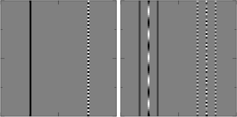
FIG. 1.: Left: Wigner function of a computational state of $5$ qubits –black (white) correspond to positive (negative) values–. The oscillating strip arises from the periodic boundary conditions. Right: Wigner function for a superposition of two computational states has two positive strips, an intermediate oscillating one and three other strips arising from the interference between the above and their mirror images.

Existing quantum algorithms are a complicated combination of classical and quantum operations that, in general, may not have a simple phase space representation. However, there are remarkable exceptions: For example, the discrete Fourier transform ${\cal U}_{FT}$, which plays a major role in quantum algorithms [3], has a very simple phase space representation (this is not surprising since the very notion of conjugate variables relies on ${\cal U}_{FT}$). In fact, the Fourier transform is represented in phase space by a dynamical map whose action is $W^{\prime}(q,p)=W(-p,q)$ (the Wigner function of the state after applying ${\cal U}_{FT}$ is obtained from the original one by changing the phase space point $(q,p)$ into $(-p,q)$, a canonical transformation that corresponds to a $\pi/2$–rotation in phase space). Another important example of a quantum algorithm with a simple phase space representation is Grover’s quantum search whose phase space action is shown in Figure 3. In such Figure we display the Wigner function of the quantum state of a computer after every iteration of Grover’s search algorithm. Our system has an $N=32$–dimensional Hilbert space (i.e., the computer has just $5$ qubits) and the algorithm is designed to search for the marked item which we chose here to be $q=16$ (indicated with an arrow in the plot). The initial state is chosen to be an equally weighted superposition of all computational states which, for the purpose of making the plots more visible, we chose to be a non-zero momentum state (the usual choice for the initial state in Grover’s algorithm is a zero momentum state but the algorithm works as well with an initial state with nonzero momentum).

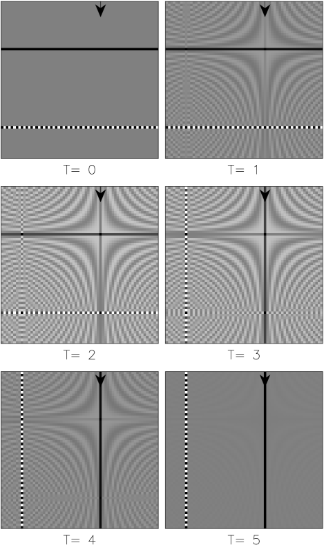
FIG. 2.: Phase space representation of Grover’s algorithm. The computer starts in a pure momentum state and evolves (after only five iterations) into a position eigenstate corresponding to the searched item.

One clearly observes that the algorithm is very simple when seen from a phase space representation. The initial state has a Wigner function which is a horizontal strip (with its oscillatory companion). After each iteration $W(q,p)$ shows a very simple Fourier-like pattern and becomes a pure coordinate state at the end of the search (in our case, the optimal number of iterations is $T\approx\pi\sqrt{N}/4\approx 5$). This representation shows that, as a map, Grover’s algorithm has a fixed phase space point with coordinate equal to the marked item ($q=16$ in our case) and momentum equal to the one of the initial state.

We have presented a method to represent both the states and the evolution of a finite quantum system in phase space. The method has points of contact, and also differences, with previous [5, 6, 8, 9] and more recent approaches [10]. The main difference that arises with respect to the usual continuous infinite dimensional case is the fact that finite dimensionality (and periodic boundary conditions implicit in modulo $N$ arithmetic) produces a characteristic interference pattern between a “fundamental” Wigner function and its periodized images (clearly illustrated in the Figures). Such fringes, that can also be interpreted as arising from the characteristic aliasing implicit in the discrete Fourier transform, are absolutely essential to provide the correct marginal distributions from the Wigner function. Finally, regarding potential applications to study quantum algorithms, we believe that this method provides a novel way to analyze their behaviour both in the computational and the complementary Fourier transformed basis, thus paving the way for a semiclassical analysis of algorithms. This work was supported by grants from Anpcyt (PICT 01014), Ubacyt and Conicet.

REFERENCES

- [1] M. Hillery, R.F. O’Connell, M.O. Scully, E. P. Wigner, Phys. Rep.106 (1984), 121.
- [2] see for example W. H. Zurek, Physics Today 44, (1991) N 10, 36; J. P. Paz, S. Habib and W. H. Zurek, Phys. Rev. D47 (1992) 488.
- [3] ”Quantum Information and Computation”, I. Chuang and M. Nielsen (2000), Cambridge University Prese.
- [4] W. K. Wooters, Ann. Phys. NY 176 (1987), 1
- [5] A. Rivas, A. M. Ozorio de Almeida, Ann.Phys. 276 (1999), 123
- [6] A. Bouzouina, S. De Bievre, Comm. Math. Phys. 178 (1996)83
- [7] J. Schwinger, Proc. Nat. Acad, Sci.46 (1960), 570, 893.
- [8] J. H. Hannay, M. V. Berry, Physica 1D (1980), 267
- [9] D.Galetti, A.F.R. Toledo Piza PhysicaA185 (1993),513
- [10] for some recent work related to discrete Wigner functions see: A. Takami et al hep-lat/0010002 and also D. Gottesman, A. Kitaev and J. Preskill, quant-ph/0008040.