Decoherence in a classically chaotic quantum system: entropy production and quantum–classical correspondence

Abstract

We study the decoherence process for an open quantum system which is classically chaotic (a quartic double well with harmonic driving coupled to a sea of harmonic oscillators). We carefully analyze the time dependence of the rate of entropy production showing that it has two relevant regimes: For short times it is proportional to the diffusion coefficient (fixed by the system–environment coupling strength). For longer times (but before equilibration) it is fixed by dynamical properties of the system (and is related to the Lyapunov exponent). The nature of the transition time between both regimes is investigated and the issue of quantum to classical correspondence is addressed. Finally, the impact of the interaction with the environment on coherent tunneling is analyzed.

2

I Introduction

The process of decoherence has been identified as one of the main ingredients to explain the origin of the classical world from a fundamentally quantum substrate [1, 2]. In fact, according to the decoherence paradigm, classicality is an emergent property imposed upon open systems by the interaction with an external environment. In all realistic situations this interaction, as it became clear in recent years, generates a de facto superselection rule that prevents the stable existence of most of the states in the Hilbert space of the system. Only a small set of states of the system are relatively stable, they are the so–called pointer states[3, 4]. While pointer states are minimally disturbed by the interaction with the environment, coherent superpositions of such states are rapidly destroyed by decoherence. Thus, this process transforms the quantum state of the system into a mixture of pointer states. In recent years the study of the physics of decoherence has helped to clarify many interesting features of this process. For example: the nature of the decoherence timescales is now well understood [5, 6]; the essential features of the process by which the pointer states are dynamically selected by the environment are well understood [7, 8, 9] (see [10] for a recent review). Moreover (and most notably) the study of decoherence became active from the experimental point of view where the first generation of experiments exploring the fuzzy boundary between the quantum and the classical world are already starting to produce interesting results [11, 12, 13].

Over the course of these studies it became clear that the decoherence process has very peculiar features for quantum systems whose classical analogues are chaotic. In fact, for such systems decoherence seems to be absolutely essential to restore the validity of the correspondence principle violated for very short times (the breakup time depends logarithmically on the Planck constant)[14, 15, 16, 17]. The reason for the breakdown of the correspondence principle for chaotic systems (and for its restoration due to decoherence) can be understood as follows: For these type of systems, quantum evolution continuously generates a coherent spreading of the wave function over large scales both in position and momentum. Thus, a classically chaotic Hamiltonian generates a quantum evolution which typically produces “Schrödinger cat” type states, i.e. starting from a state which is well localized both in position and momentum the quantum evolution produces a state which is highly delocalized exhibiting strong interference effects. One may be tempted to argue that this effect, while existing, could not be relevant for large macroscopic systems. But, surprisingly or not, even for as large an object as the components of the solar system which are chaotic, quantum predictions are alarming: On a timescale $t_{\hbar}$ as short as a month for Hyperion, one of the moons of Saturn whose chaotic tumbling motion has been analyzed [18], the initial Gaussian state of this celestial body would spread over distances of the order of the radius of its orbit![15]. Thus, though planetary dynamics appears to be a safe distance away from the quantum regime, as a consequence of the chaotic character of the evolution, a simple application of the Schrödinger equation would tell us that this is not the case. In fact, the macroscopic size of a system (be it a planet or a cat) is not enough to guarantee its classicality. Thus, classicality in such system would emerge only as a consequence of decoherence, as we will later discuss in this paper.

The reason why a classically chaotic Hamiltonian generates highly nonclassical states can be related to the fact that chaotic dynamics is characterized by exponential divergence of neighboring trajectories. To be able to present this argument, based on the notion of trajectories, it is better to formulate quantum mechanics in phase space (a task that can be accomplished by using, for example, the Wigner distribution [19] to represent the quantum state). In fact, if one prepares a quantum system in a classical state, with a Wigner function well localized in phase space and smooth over regions with an area which is large compared with the Planck constant, it will initially evolve following classical trajectories in phase space. Therefore, after some characteristic time the initially smooth wave packet will become stretched in one (unstable) direction and, due to the conservation of volume, squeezed in the other (stable) one. This squeezing and stretching is also accompanied by the folding of classical trajectories which, in the fully chaotic regime, tend to fill all the available phase space. The combination of these three related effects – squeezing, stretching and folding – forces the system to explore the quantum regime. Thus, being stretched in one direction the wavepacket becomes delocalized and, as a consequence of folding, quantum interference between the different pieces of the wavepacket, which remain coherent over long distances, develops. The timescale for the correspondence breakdown can be also estimated via a simple argument: As the wave packet squeezes exponentially fast in one direction (momentum, for example), $\sigma_{p}(t)=\sigma_{p}(0){\rm e}^{-\lambda t}$, it will correspondingly become coherent over a distance that can be estimated from Heisenberg’s principle as $l(t)\geq\frac{\hbar}{\sigma_{p}(0)}{\rm e}^{\lambda t}$. When the spreading is comparable with the scale $\chi$ where the potential is significantly nonlinear, folding will start to appreciatively affect the evolution of the wave packet and long range quantum interference will set in. This time, which corresponds approximately to the time when quantum and classical expectation values start to differ from each other, can therefore be estimated as $t_{\hbar}=\lambda^{-1}{\rm ln}(\frac{\sigma_{p}(0)\chi}{\hbar})$ (note that the quantity $\chi$ can be as large as the size of the orbit of a planet [15, 20] for gravitational potential).

But nothing of this sort is evident in real life: the moon of Saturn does not spread over large distances and the correspondence principle seems to be valid for macroscopic objects that, like Hyperion, behave according to classical laws. So, how can classical mechanics be recovered? Decoherence is a way out of this problem. As the system evolves while continuously interacting with its environment, it may become classical if the interaction is such that it continuously destroys the quantum coherence which are dynamically generated by the chaotic evolution. The role of decoherence in recovering the correspondence principle has been suggested some time ago [15] and numerically analyzed more recently [16].

But, as originally suggested by Zurek and one of us [14], the decoherence process for classically chaotic systems has another very important feature, that comes as a bonus. The interaction with the environment destroys the purity of the system since they become entangled. Thus, information initially stored in the system leaks into the environment and therefore decoherence is always accompanied with entropy production. This is, of course, true both for classically regular and classically chaotic systems. But what distinguishes chaotic systems is the existence of a robust range of parameters for which the rate at which the information flows from the system into the environment (i.e., the rate of entropy production) becomes entirely independent of the strength of the coupling between the system and the environment and is dictated by dynamical properties of the system only (i.e., by averaged Lyapunov exponents). The reason for this can also be understood using a simple (clearly oversimplified) argument. The decoherence process destroys quantum interference between distant pieces of the wave packet of the system and puts a lower bound on the small scale structure that the Wigner function can develop. Thus, the Wigner function can no longer squeeze indefinitely but it stops contracting as a consequence of the interaction with the environment, which can be typically modelled as diffusion [22, 23, 24]. As a consequence of this, and due to the fact that expansion (or folding) is not substantially affected by diffusion, the entropy of the system grows at a rate which is essentially fixed by the average rate of expansion given by the average Lyapunov exponent. In this regime, the entropy production rate becomes independent of the diffusion constant (which, on the other hand, is responsible for the whole process). This result was first conjectured in [14]. More recently, numerical evidence supporting the conjecture was presented [17, 25, 26, 27, 28]. The aim of this paper is to present solid numerical evidence supporting this result and to study other related aspects of decoherence for a particular chaotic system. As will become clear later, our studies show that the time dependence of the entropy production rate has two rather different regimes. First, there is an initial transient where the entropy production rate is proportional to the system–environment coupling strength (i.e., in this initial regime the rate behaves in the same way as in the regular –non chaotic– case). Second, after this initial transient the entropy production rate goes into a regime where its value is fixed as conjectured in [14] by the Lyapunov exponents of the system and is independent of the strength of the coupling to the environment. In our work we show that the transition time $t_{c}$ between both regimes is linearly dependent on the entropy of the initial state, and logarithmically dependent on the system–environment coupling strength.

Our aim in this paper is not to give an extensive list of all relevant references connected to the study of dissipative effects in classically chaotic quantum systems. However, we believe it is worth pointing out that our work is by no means the first attempt to study these effects which, in connection to problems such as the impact of noise on localization, the appearence of classical features in phase space (like strange attractors, etc) were studied in pioneering works several years ago (see for example [29]). As general source of reference in this area we recommend to interesting books where one can find a rather extended compilation of important works [30, 31]. For our numerical study we have chosen as nonlinear system the driven quartic double well, described in detail in Section II. We study the evolution of our system for very simple (Gaussian) initial conditions (i.e., initial conditions that, from a start, do no exhibit any quantum interference effects) so as to focus our attention on the interplay between two competing effects: generation and destruction of dynamically generated interferences. We also present, in Section II, a discussion of the breakdown of correspondence for chaotic systems. Then, on Section III the way in which we model the interaction between our system and an environment is presented with some detail. We do this by using two complementary approaches based on master equations both giving consistent results but one of them enable the study of the evolution for long dynamical times, which is relevant for discussing the impact of decoherence on tunneling. Numerical results concerning the time dependence of the decoherence rate and a discussion of their relevance are presented in Section IV. Finally, we discuss the impact of the interaction with the environment on the tunneling phenomena in Section V and we end with some concluding remarks on Section VI.

II Evolution of the quantum isolated system

In this Section we study the dynamical behaviour of an isolated quantum system with Hamiltonian

$$H_{0}(x,p,t)\,=\,\frac{p^{2}}{2m}\,-\,bx^{2}\,+\,\frac{x^{4}}{64a}\,+\,sx\cos(\omega t),$$ (1)

which corresponds to a harmonically driven quartic double well. This non-linear system has been extensively studied [32, 33] in the literature. For $s=0$ the system is integrable and exhibits the generic phase space of a bistable system. It has two stable fixed points at $x=\pm\sqrt{(}32ba),\ p=0$ (with associated energy $E=-16b^{2}a$) and one unstable fixed point at $x=0,\ p=0$ (with $E=0$). The presence of the driving term introduces an infinite number of primary resonance zones in the phase space of the system. The tori near the separatrix of the non-driven system ($E=0$) and KAM invariant tori in the region between resonance zones are progressively destroyed as the amplitude $s$ of the driving increases. The phase space of the system starts to look chaotic, presenting in general a mixed nature as can be seen (for two sets of parameters) in Figure 1. The regions around the two stable fixed points and the chains of resonant islands form regular regions where the dynamics of the system is nearly integrable. The chaotic layers between regular regions develop from the homoclinic tangles, the intrincated interweaving of the stable and unstable manifolds originated at the hyperbolic fixed points between the resonant islands or the one at the origin. For small values of the driving amplitude, chaotic layers are so thin that only those near the unstable fixed point of the integrable system can be seen in the stroboscopic phase space portrait. As the value of $s$ is increased these chaotic regions gain in relevance while resonances other than the two first ones near the stable fixed points become in turn smaller and are almost invisible to the eye. For large values of the driving amplitude $s$ the different chaotic layers merge into what is called the chaotic sea; the stable islands and two first resonant islands are much reduced (see Figure 1a). In what follows we will choose parameters so that either the majority of the phase space is chaotic, as in Figure 1b, where the stable islands around the stable fixed points of the integrable system have shrunken to invisibility and only the two first resonance islands are seen, or the regular regions coexist with the chaotic sea as shown in Figure 1a.

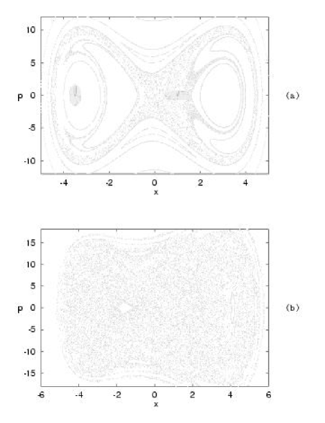
FIG. 1.: Stroboscopic phase space of the driven double well with parameters (a) $m=1$, $b=10$, $a=1/32$, $s=1$, $\omega=5.35$ and (b) $m=1$, $b=10$, $a=1/32$, $s=10$, $\omega=6.07$. The borders of the dark elipses represent contours of minimun uncertainty Gaussian initial conditions at 1/20 of its peak value, for $x_{0}=-3.7$, $p_{0}=0$, $\sigma_{x}=.05$, $\sigma_{p}=1$ on the leftmost island and $x_{0}=1$, $p_{0}=0$, $\sigma_{x}^{2}=.05$, $\sigma_{p}^{2}=.05$ on the chaotic sea.

As we mentioned above, our aim is to follow the quantum evolution of initial states whose Wigner functions are fully contained either in a regular island or in the chaotic sea, as illustrated in Figures 1a and 1b. This requirement forces us to take values of $\hbar$ which are small enough. Indeed, for the parameter set corresponding to Figure 1a, the leftmost regular island has an area which is approximately given by ${\cal A}\sim 6\pi$. If we need states well localized within each region (the regular islands or the chaotic sea) we need to compare this area with the one covered by the dark ellipses appearing in Figure 1, which are given by ${\cal A}_{e}=2\pi\ln(20)\sigma_{x}\sigma_{p}=\pi\ln(20)\hbar$ (i.e., we consider initial states which are pure, minimal uncertainty, coherent states). Thus, a reasonable value for $\hbar$ (the one we choose) is $\hbar=0.1$ for the island to be about 20 times larger than the extent of the initial state (for the parameters corresponding to Figure 1b a larger value of $\hbar$ could also be chosen for our purposes). + We numerically solved the Schrödinger equation for this system evolving the above initial states using two different methods. First, we integrated this equation with a step by step algorithm using a high resolution spectral method [34]. Second, we solved the same equation applying a numerical technique based on the use of Floquet states [35]. This method consists of numerically finding eigenstates of the unitary evolution operator for one period (Floquet states) which form a complete basis of the Hilbert space of the system. By expanding the initial state on this basis, the solution of the Schrödinger equation becomes trivial[36]. Thus, all the difficultly of the method is hidden in finding the Floquet states (the same applies when solving the Schrödinger equation for a time–independent Hamiltonian). We succesfully used this method for some parameter sets but did not apply it for all cases of interest. In fact, the main difficulty of the method is the number of Floquet states required to accurately expand the initial states shown in Figure 1, which rapidly grow as $\hbar$ becomes small (for example, for the parameters of Figure 1b, with $\hbar=0.1$, one needs more than $200$ Floquet states to evolve the wave packet centered in the chaotic sea). In what follows we will discuss the typical results one finds when solving the Schrödinger equation with the above initial states.

A Initial states in a regular island

The time series of the expectation value of the position $x$ of the particle both for classical and quantum evolutions, for the initial Gaussian state located within the leftmost regular island as shown on Figure 1a can be seen in Figure 2. Notice that the state is centered at $x_{0}=-3.7,p_{0}=0$ and that its variances are $\sigma_{x}=.05,\sigma_{p}=1$. Classical and quantum expectation values remain identical within the numerical errors of our calculations, in agreement with previous results [33, 37]. Similar results were found for higher order moments of $x$ and $p$ and for different initial conditions embedded either in the stable or the resonant islands and for different sets of parameters of the system. These results can be understood as follows: When the initial Gaussian function is located within a regular island, its Floquet decomposition is characterized by a small number of states, mostly localized on the regular regions. Thus, only very few frequencies enter into play in the dynamics and the time series of the expectation value of any observable appears as quasi periodic and regular. Moreover, as the Floquet states entering in the decomposition of the initial state are localized on integrable tori, EBK quantization is possible and both classical and quantum expectation values (and distribution functions) look identical for long time scales. Breakdown of correspondence is expected on time scales inversely proportional to some power of $\hbar$ [38], which is sufficiently slow to cause no difficulties with the classical limit of quantum theory.

FIG. 2.: Time series of the classical and quantum expectation value of $x$ for the states drawn on Fig.1a.

Nevertheless, as localized Floquet states come from the superposition of almost degenerate symmetry-related pairs (doublets), each belonging to a different parity class, the quantum particle will eventually tunnel through the chaotic sea into the related regular island [33, 39, 40] while for the classical particle this feature is forbidden. Tunneling times are very long for the parameters we chose (typically they are of the order of $50$–$100$ times the driving period). The accumulation of error makes step by step integration of the Schrödinger equation troublesome to study this tunneling regime. However, a solution based on Floquet states is more convenient since it allows us to compute the state at any time provided we know it within the first period $\tau$, with $\tau=2\pi/\omega$ [40, 41, 42]. We applied this method for several sets of parameters chosen in such a way that the number of Floquet states needed to faithfully represent the Hilbert space doesn’t become too large (still enabling us to keep states well localized within the regular island). One of the parameter sets we used for this purpose is $m=1$, $b=10$, $a=1/32$, $s=4$, $\omega=5.35$ and $\hbar=1$. The stroboscopic phase space looks like something in between Figures 1a and 1b but the value of $\hbar$ is ten times larger than the one used in the above Figure. For this parameter set, Figure 3 shows the evolution of the expectation value of the position for an initial state located in the leftmost regular island, centered at $x_{0}=-3.52$, $p_{0}=0$ (with $\sigma_{x}=0.25$, $\sigma_{p}=2$). This initial state was expanded by 20 Floquet states. In this case we clearly see the system tunnel from one regular island to the other one (deviation from classical behavior is observed for times well below the tunneling time, which in this case of the order of $t=56\tau$).

FIG. 3.: Time series of the quantum (full line) and classical (dotted line) expectation value of $x$ for an initial state located within a regular island (see text).

The evolution of quantum and classical distribution functions is shown in Figure 4 for two different times: a time half way the tunneling ($t=28\tau$) where the wave packet is completely delocalized, and the time for which the state has tunneled to its pair related regular island on the right ($t=56\tau$). Notice that though the state is initially peaked in the leftmost regular island, there is a nonnegligible probability of finding it on the chaotic sea, due to the relatively high value of $\hbar$. For this reason, the tail of the initial Gaussian distribution spreads over the whole chaotic sea as time goes on. For the classical case, this effect is not very important since the state stays within the regular island. On the contrary, for the quantum evolution, one clearly observes the wave packet tunneling through the chaotic sea into the pair related regular island on the right.

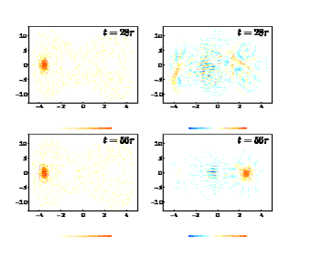
FIG. 4.: The classical (left) and quantum (right) evolution of the phase space distribution function for the tunneling case. Parameters are that of Fig. 3.

B Chaotic states

For Gaussian states initially located within the chaotic sea, as the one corresponding to the ellipse in Figure 1a, the behaviour is quite different from that of the regular initial state. In fact, Figure 2 shows the time series of the quantum and classical expectation values of the position for this initial state. We see that after a time scale much shorter than that of the regular case (our results are consistent with a logarithmic dependence of this time scale on $\hbar$), discrepancies between classical and quantum predictions are evident. For the various different initial conditions and parameters of the system tested, breakdown of correspondence occurs at very early times, and in all cases it is comparable with the dynamical scale $\tau$. Apart from the noticeable deviation between quantum and classical predictions one clearly sees that the expectation values have a much more irregular behavior than in the integrable case. This is expected and, in the quantum regime, can be explained as due to the fact that the number of Floquet states required to expand the initial state is, contrary to the regular case, rather large. Thus, as Floquet states are mostly extended over the whole chaotic sea (all the more in the semiclassical limit) the evolution of the initial Gaussian state will contain many more frequencies (a few hundred, typically) and as a consequence of this the time evolution of any expectation value looks rather irregular. The deviation between classical and quantum expectation values is just a consequence of the fact that the quantum state, described in the phase space by the Wigner function, becomes more and more different from the corresponding classical distribution function [16]. This situation is illustrated in Figure 5 where we show the Wigner distribution function for the above initial Gaussian state (localized in the chaotic sea), compared with the corresponding classical distribution function for four different times. Very quickly – even before classical and quantum expectation values deviate from each other –the quantum distribution function becomes affected by small scale interference effects, and develops into a highly non-classical distribution function. This results are also in agreement with previous ones [33, 37].

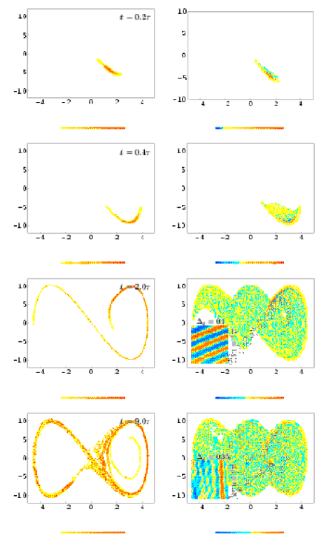
FIG. 5.: Classical (left) and quantum (right) distribution functions for four different times. Already for early times interference effects are observed, but after $t\sim 2\tau$ they sprout over the whole available phase space and go down to very small scales, as shown by the insets of area $\hbar$, which blow-up the tiny rectangles drawn on the Wigner functions for $t=2\tau$ and $t=9\tau$.

For our purposes it is very useful to represent the temporal evolution of quantum states in phase space. The time dependence of the Wigner function (shown in Figure 5), is goverened, in general, by an equation entirely equivalent to Schrödinger equation, which can be written as:

$$\dot{W} = \left\{H_{0},W\right\}_{PB}+$$ (2)

$$+ \sum_{n\geq 1}{(-1)^{n}(\hbar/2)^{2n}\over{(2n+1)!}}\partial_{x}^{(2n+1)}V\partial_{p}^{(2n+1)}W.$$ (3)

In this equation, the first term on the right hand side is the Poisson bracket that generates purely classical evolution. The second term, containing higher odd derivatives, is responsible for the quantum corrections [19, 37]. The fate of the Wigner function can be understood qualitatively by using the following simple argument [14]: If one starts from an initial state which is smooth (as the ones shown in Figure 1), the higher derivatives terms are negligible and the Poisson bracket term dominates. Therefore, the Wigner function will tend to follow initially the Liouville flow, i.e., it will evolve following the classical trajectories. As any point in the chaotic sea is hyperbolic, the initially regular patch will stretch along the unstable manifold and squeeze in the other – stable – direction. As the Wigner function squeezes, its derivative will tend to grow and, consequently, quantum corrections will tend to become more and more important. The time scale for which quantum corrections must be taken into account can be estimated as $t_{\hbar}=\lambda^{-1}\ln(\chi\sigma_{q}(0)/\hbar)$ [14] where $\chi$ is the scale where the nonlinearities of the potential come into play and is usually defined as $\chi=(\partial_{x}V/\partial_{x}^{3}V)^{1/2}$ ($\sigma_{q}(0)$ is the initial spread of the distribution function in the stable manifold and $\lambda$ is the Lyapunov exponent of the system). Moreover, as the motion is bounded, the Wigner function will eventually tend to fold and so different pieces will coherently interfere making the distribution function develop small scale structure as seen in Figure 5. The scale at which structure will tend to develop is typically sub–Planckian: thus, as we will have $\delta p=\hbar/L$ and $\delta x=\hbar/P$ (where $L$ and $P$ are the size of the system in position and momentum), the region over which the Wigner function will tend to oscillate has an area approximately given by ${\cal A}\approx\hbar^{2}/LP=\hbar\times(\hbar/LP)\ll\hbar$ [43]. In our simulations we verified that, after a time consistent with $t_{\hbar}\approx 0.5\tau$, for the set of parameters here considered, the quantum phase-space distribution does not resemble the classical one and the Wigner function oscillates wildly on tiny scales of size $\delta p\approx.01$ and $\delta x\approx.005$ (being the product of the order of ${\cal A}=\delta p\delta x\approx 5\times 10^{-5}\ll\hbar$). The insets on Figure 5 show the development of small scale structure on the Wigner functions for relevant times. There, a detail of the distribution function over a region of area $\hbar$ is shown. The existence of this sub–Planckian structure in the Wigner distribution has been overlooked in the literature and its relevance has only been noticed recently [43].

III Coupling to the environment: master equations

Here we will describe the way in which we analyze the evolution of our system when it is coupled to an environment. The role of such environment will be played in our case by an infinite number of oscillators coupled to the system via an interaction term in the Hamiltonian, which is assumed to be bilinear both in the coordinates of the system and the oscillators. As we are interested in following the evolution of the system solely, we will compute the reduced density matrix $\rho$ obtained from the full density matrix of the Universe (system$+$environment) by taking the partial trace over the environment $\rho=Tr_{E}(\rho_{U})$, where $\rho_{U}$ is the full density matrix of the Universe. This reduced density matrix will obey a master equation which can be obtained from the full von–Neumann equation by tracing out the environment. There is a vast literature dealing with the properties of the master equation obtained under a variety of assumptions. Our purpose here is not to present a review of these results but to sketch the basic method used to obtain the master equations we will use for our studies below (see [10] for a more extensive review on the derivation and properties of master equations in studies of decoherence).

The general approach to obtain the master equation is the following: We model the environment by a set of harmonic oscillators with mass $m_{i}$ and natural frequency $\omega_{i}$, in thermal equilibrium at temperature T. The Hamiltonian is $H_{R}=\sum_{i}\omega_{i}\;(b_{i}^{{\dagger}}b_{i}+1/2)$, where $b_{i}$ and $b_{i}^{{\dagger}}$ are the annihilation and creation operators, respectively, for a boson mode of frequency $\omega_{i}$. We further assume that the interaction Hamiltonian between the system and the environment is $H_{I}=\;x\;\sum_{i}(g_{i}\,b_{i}+g_{i}^{*}\,b_{i}^{{\dagger}})$, where $g_{i}$ are coupling constants.

The evolution of the reduced density matrix of the particle can be obtained by taking the partial trace over the environment of the exact von Neumann equation for the full Hamiltonian, that reads $\rm{i}\,\hbar\,\dot{\rho_{U}}=[\,H(t)\,,\rho_{U}]$. This can be straightforwardly done under a number of standard assumptions (see [10] for more details): First, one assumes that the system and the environment are initially uncorrelated and that the reservoir is in an initial state of thermal equilibrium at some temperature $T$. Second, one assumes that the system and the environment are very weakly coupled. So, solving the von Neumann equation perturbatively in the interaction picture (up to second order in perturbation theory) a master equation for the reduced density operator is obtained, which fully determines the quantum dynamics of our system. It reads:

$$\dot{\rho}(t) = -\int_{0}^{t}{dt^{\prime}\;g_{S}(t-t^{\prime})\;[\,x(t)\,,[\,x(t^{\prime})\,,\rho(t)\,]\,]}\;+$$ (4)

$$+ \imath\,\int_{0}^{t}{dt^{\prime}\;g_{A}(t-t^{\prime})\;[\,x(t)\,,\{\,x(t^{\prime})\,,\rho(t)\,}\,\}]\;,$$ (5)

where the above kernels are

$$g_{S}(t-t^{\prime}) = \;\sum_{i}|g_{i}|^{2}(1+2n(\omega_{i}))\cos(\omega_{i}(t-t^{\prime}))\;,$$ (6)

$$g_{A}(t-t^{\prime}) = \;\sum_{i}|g_{i}|^{2}\sin(\omega_{i}(t-t^{\prime}))\;,$$ (7)

with $n(\omega)=\frac{1}{{\rm e}^{\beta\hbar\omega}-1}$ (and $\beta=1/k_{B}T$). It is worth stressing that the above master equation is derived without appealing to the usual Markovian approximation (see [10, 22]). However, in our studies we restrict ourselves to the Markovian regime where the kernels (6) are local in time. We solved the above master equation for two different regimes and environmental couplings. First, we considered the widely used ohmic–high temperature regime of the Brownian motion model where a simple master equation can be written and solved. Second, we obtained a master equation for the evolution of a coarse grained density matrix obtained from eq. (4) by averaging over one driving period. This can be naturally done by using the Floquet representation and is useful to study some properties of the open system in the long time regime. We will now describe the two methods.

A Ohmic–high temperature environment

The simplest special case of equation (4) follows when assuming the high temperature limit of an Ohmic environment. Defining an spectral density for the environment as $J(\omega)=\lim_{\Delta\omega\rightarrow 0}\frac{\pi}{\Delta\omega}\sum_{\omega<\omega_{i}<\omega+\Delta\omega}|g_{i}|^{2}$, assuming that the spectrum is ohmic, i.e., that $J(\omega)=\gamma m\omega/\hbar$, and going to the high temperature limit, $g_{S}(t-t^{\prime})\,=\,D\,\delta(t-t^{\prime})$ and $g_{A}(t-t^{\prime})=2\gamma\dot{\delta}(t-t^{\prime})$ with $D=2m\gamma k_{B}T$, the following well known equation for the Wigner function of the system is obtained:

$$\dot{W}=\left\{H_{0},W\right\}_{PB} + \sum_{n\geq 1}{(-1)^{n}\hbar^{2n}\over{2^{2n}(2n+1)!}}\partial_{x}^{(2n+1)}V\partial_{p}^{(2n+1)}W$$ (8)

$$+ 2\gamma\partial_{p}\left(pW\right)+D\partial_{pp}^{2}W.$$ (9)

The physical effects included in this equation are well understood: The first term on the right hand side is the Poisson bracket generating the classical evolution for the Wigner distribution function $W$; the terms in $\hbar$ add the quantum corrections. The environmental effects are contained in the last two terms generating, dissipation and diffusion, respectively. In the high-$T$ limit here considered dissipation can be ignored and only the diffusive contributions need be kept (doing this we are taking the $\gamma\rightarrow 0$ limit while keeping $D$ constant). The diffusion constant was chosen small enough so that energy is nearly conserved over the time scales of interest. Equation (9) was integrated by means of a high resolution spectral algorithm [34]. Results were stable against changes both in the resolution of phase space and the time accuracy required on each integration step. They will be presented on Section 4.

B Coarse grained master equation in the Floquet basis:

It is interesting to write equation (4) in the Floquet basis $|\psi_{\mu}(t)\rangle=\exp^{-\imath\varepsilon_{\mu}t}\;|\phi_{\mu}(t)\rangle$, where the $|\phi_{\mu}(t)\rangle$ are $\tau$-periodic, taking advantage of the $\tau$-symmetry of our system $H_{0}$. There are in the literature several approaches of the kind [39, 40, 41, 42]. Ours is similar to that of Kohler et. al. [44], though in that reference the authors have restricted the use of the equation to the study of chaotic tunneling near a quasienergy crossing. When one writes the master equation in the Floquet basis and takes the Markovian high temperature limit, the resulting equation has $\tau$–periodic coefficients. Therefore, one can derive a temporal coarse–grained equation by taking the average of such equation over one oscillation period. The resulting equation for the average density matrix in one period $\sigma$ turns out to be

$$\dot{\sigma}_{\mu,\nu}=\sum_{\alpha,\beta}M_{\mu,\nu,\alpha,\beta}\sigma_{\alpha,\beta},$$ (10)

where the coefficients $M_{\mu,\nu,\alpha,\beta}$ are defined as

$$M_{\mu,\nu,\alpha,\beta} = -\frac{\imath}{\hbar}(\varepsilon_{\mu}-\varepsilon_{\nu})\,\delta_{\alpha,\mu}\delta_{\beta,\nu}-D\,\{\delta_{\beta,\nu}\langle\langle x^{2}\rangle\rangle_{\mu,\alpha}$$ (11)

$$+ \delta_{\alpha,\mu}\langle\langle x^{2}\rangle\rangle_{\beta,\nu}-2\,\langle\langle x\rangle\rangle_{\mu,\alpha}\;\langle\langle x\rangle\rangle_{\beta,\nu}\}$$ (12)

where the notation $\langle\langle A\rangle\rangle_{\mu,\nu}=\frac{1}{\tau}\int_{t}^{t+\tau}dt^{\prime}\langle\phi_{\mu}(t^{\prime})|A|\phi_{\nu}(t^{\prime})\rangle$ is used to denote time averages of matrix elements of operators in the Floquet basis. As this is an equation with constant coefficients, once these coefficients are numerically calculated, the solution is formally obtained for all times as $\sigma_{\mu,\nu}(t)=\sum_{\alpha,\beta}\left({\rm e}^{Mt}\right)_{\mu,\nu,\alpha,\beta}\sigma_{\alpha,\beta}(0)$. The difficulty in solving this equation resides on the large number $n$ of Floquet states one typically needs to accurately represent a state located in the chaotic sea (as we mentioned above, a semiclassical argument to estimate the number of such states is given by the ratio ${\cal A}/(2\pi\hbar)$, where ${\cal A}$ is the area of the chaotic sea, which might quickly become a very large number). As $M$ has dimension $n^{4}$, numerical limitations spring up at this point. However, for some parameter values it was still possible to manage the numerical problem. The results will be presented on Section V.

IV Results

Before going into a detailed description of our model for the open system it is instructive to analyze equation (9) so as to have an intuitive idea of what is going on. When the diffusion term is absent –that means, states evolve simply according to Schrödinger equation– for a smooth initial state the dominant term is the Poisson bracket. As we already discussed in Section 2, the Wigner function initially evolves following nonlinear classical trajectories, looses its Gaussian shape and develops tendrils while folding. If the initial state is located in the chaotic sea, this happens exponentially fast. Due to the combination of squeezing-stretching and folding the gradients increase and quantum corrections in equation (9) become important, so discrepancies between quantum and classical predictions begin to be relevant. Also, quantum interferences among different pieces of the wave packet develop and generate oscillations in the Wigner function.

The effect of the decoherence producing term in equation (9) can be understood as being responsible of two interrelated effects: On the one hand, the diffusion term tends to wash out the oscillations in the Wigner function suppressing quantum interferences. Thus, for this system decoherence is the dynamical suppression of the interference fringes that are dynamically produced by nonlinearities. The time–scale characterizing the disappearance of the fringes can be estimated easily using previous results [6]: Fringes with a characteristic wave vector (along the $p$–axis of phase space) $k_{p}$ decay exponentially with a rate given by $\Gamma_{D}=Dk_{p}^{2}$. Noting that a wave packet spread over a distance $\Delta x$ with two coherently interfering pieces generate fringes with $k_{p}=\Delta x/\hbar$ one concludes that the decoherence rate is $\Gamma_{D}=D\Delta_{x}^{2}/\hbar^{2}$. This rate depends linearly on the diffusion constant. When the Wigner function is coherently spread over the whole available phase space one expects fringes with wavelength of the order of $1/L$ where $L$ is the size of the system (these are responsible for the existence of sub–Planck structure in the Wigner function, as mentioned in Section 2). The rate at which these fringes disappear due to decoherence is then $\tilde{\Gamma}_{D}=DL^{2}/\hbar^{2}$. Thus, we can derive a condition that should be satisfied in order for these fringes to be efficiently destroyed by decoherence: the destruction of the fringes, that takes place at a rate $\tilde{\Gamma}_{D}$, should be faster than their regeneration, that takes place at a rate $\Omega_{f}$ fixed by the system’s dynamics and related both to the Lyapunov time and the folding rate. Thus, if $\Omega_{f}\ll\tilde{\Gamma}_{D}$ the small scale fringes will be efficiently washed out and the Wigner function would remain essentially positive. It is worth mentioning that the destruction of fringes would generate entropy at a rate which, provided the condition $\Omega_{f}\ll\tilde{\Gamma}_{D}$ is satisfied, should be independent of the diffusion constant, and should be fixed by $\Omega_{f}$. Thus, one could argue that every time the Wigner function stretches and folds, becoming an approximate coherent superposition of two approximately orthogonal states, the destruction of the corresponding fringes should generate about one bit of entropy. If the timescale for the fringe disappearance ($\tilde{\Gamma}_{D}$) is much smaller than the one for producing the above superposition (fixed by $\Omega_{f}$) then the entropy production rate would be simply equal to $\Omega_{f}$ (ideally, one would expect one bit of entropy created after a time $1/\Omega_{f}$).

However, the disappearance of the interference fringes is not the only effect produced by decoherence. There is a second related consequence of this process (which is also present in the classical case): While interference fringes are being washed out by decoherence, the diffusion term also tends to spread the regions where the Wigner function is possitive, contributing in this way to the entropy growth. But, as discussed in [14, 28], the rate of entropy production distinguishes regular and chaotic cases. For regular states, decoherence should produce entropy at a rate which depends on the diffusion constant $D$. However, for chaotic states the rate should become independent of $D$ and should be fixed by the Lyapunov exponent. The origin of this $D$-independent phase can be understood using a simple minded argument (presented first in [14] and later discussed in a more elaborated way in [28]): Chaotic dynamics tends to contract the Wigner function along some directions in phase space competing against diffusion. These two effects balance each other giving rise to a critical width below which the Wigner function cannot contract. This local width should be approximately $\sigma_{c}^{2}=2D/\lambda$ (being $\lambda$ the local Lyapunov exponent). Once the critical size has been reached, the contraction stops along the stable direction while the expansion continues along the unstable one. Therefore, in this regime the area covered by the Wigner function grows exponentially in time and, as a consequence, entropy grows linearly with a rate fixed by the Lyapunov exponent. Moreover, the appearance of a lower bound for the squeezing of the Wigner function make quantum corrections unimportant and so the Wigner function will evolve classically (following Liouville flow plus diffusive effects), and the correspondence will be reestablished.

In this Section we present solid numerical evidence supporting the existence of this $D$-independent phase. For simplicity, instead of looking at the von Neumann entropy ${\cal H}_{VN}=-Tr\left(\rho_{r}\log\rho_{r}\right)$ we examine the linear entropy, defined as ${\cal H}=-\log(Tr\left(\rho_{r}^{2}\right))$, which is a good measure of the degree of mixing of the system and sets a lower bound on ${\cal H}_{VN}$ (i.e, one can show that ${\cal H}_{VN}\geq{\cal H}$). The above argument concerning the role of the critical width $\sigma_{c}$ may appear as too simple but captures the essential aspects of the dynamical process. We can present a more elaborate argument using the master equation (9) to show that the rate of linear entropy production can always be written as:

$$\dot{\cal H}=2D\langle(\partial_{p}W)^{2}\rangle/\langle W^{2}\rangle,$$ (13)

where the bracket denotes an integral over phase space. The right hand side of this equation is proportional to the mean square wave–number computed with the square of the Fourier transform of the Wigner function. This implies that the entropy production rate is closely related to the phase space structure present in the Wigner distribution. Thus, the $D$–independent phase begins at the time when the mean square wave–length along the momentum axis scales with diffusion as $\sqrt{D}$ (as $\sigma_{c}$ does). This behavior cancels the diffusion dependence of $\dot{\cal H}$ which becomes entirely determined by the dynamics.

Appart from analyzing the $D$–independent phase of entropy production we analyze the nature of the the transition between the diffusion dominated to the chaotic regime. This time $t_{c}$ can also be estimated along the lines of the previous argument: The time for which the spread of the Wigner function approches the critical one is $t_{c}\approx\lambda^{-1}\log(\sigma_{p}(0)/\sigma_{c})$. According to this estimate $t_{c}$ should depend logarithmically on the diffusion constant and on the initial spread of the Wigner function (for Gaussian initial states the spread depends exponentially on the initial entropy, therefore $t_{c}$ should vary as a linear function of the initial entropy). Our numerical work is devoted to testing these intuitive ideas.

In the following subsections we present our results. First, we will show (for completeness of our presentation) how decoherence restores classicality washing out interference fringes. Then, we focus on our main goal: the study of the entropy production rate of the system as a function of time.

A Correspondence principle restored: disappearance of interference fringes

In Section 2B we showed how classical and quantum expectation values of the position observable become different from each other after a relatively short time when the initial state is located within the chaotic sea. In Figure 6 we show how this result is affected by decoherence. There one observes the time dependence of the expectation value of position obtained by solving the master equation (9) (i.e., considering the decoherence effect) as compared with the corresponding classical time series. It is clear that, in accordance with results previously obtained in [16], the correspondence principle has been restored.

FIG. 6.: Time series of the classical and quantum expectation value of $x$ for the states drawn on Figure 1a, for the open system ($D=0.01$)

With respect to the behaviour of the Wigner function (shown for the case of pure Schrödinger evolution in Figure 3), the impact of decoherence on this distribution is seen in Figure 7 where we compare the decohered Wigner function with the classical distribution at three different times. It is clearly seen that decoherence in this case is strong enough to induce classicality, which is reflected at the level of the Wigner function and, consequently, at the level of any expectation value. It is worth mentioning that the condition for classicality discussed above [14, 15], i.e. $\sigma_{c}\chi\gg\hbar$, is satisfied in our case: For the parameters we are using here we have that $\sigma_{c}\approx 0.2$, $\chi\approx 4$ and therefore we are in a (not so highly) classical regime (remember that we are using $\hbar=0.1$). The small scale structure developed by the distribution fuction on the isolated evolution (Figure 5) is stopped when it reaches the lower bound $\sigma_{c}$ imposed by the environment. The insets on Figure 7 shows the portion of area ${\cal A}=3\hbar$ of the decohered Wigner function marked by the tiny rectangle for $t=9\tau$. The sub-Planckian structure observed for the isolated evolution is now absent: the interference fringes have a typical size which is above $\sigma_{c}=0.2$.

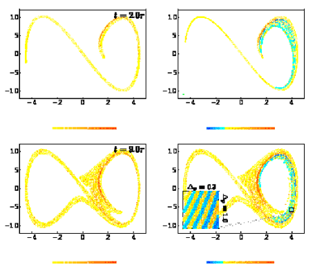
FIG. 7.: Classical (left) and quantum (right) distribution functions for the same initial condition as on Fig.5, at $t=2\tau$ and $t=9\tau$, when the system is opened to the action of the environment ($D=0.01$).

B Entropy Production

Here we study the time dependence of the entropy production rate. In Figure 8 we plot the time dependence of $\log(\frac{d\cal H}{dt})$ both for the initial condition centered in the regular island and for the one centered in the chaotic sea (the initial states are the ones corresponding to those shown in Figure 1a). Figure 8 illustrates one of the main points we want to establish in this paper. First of all one notices a drastic difference between the behaviour of the entropy production rate for regular or chaotic cases . For regular initial conditions, the entropy is always produced at a rate which is linearly dependent on the diffusion coefficient $D$ as it is clearly seen in the plot at the top of Figure 8. On the other hand, for chaotic initial conditions the behavior is completely different. For early times the rate depends linearly on $D$ but this initial regime is rapidly followed by one where the entropy production rate is independent of the value of the diffusion coefficient. The existence of the initial $D$ dependent transient for the chaotic case comes as no surprise. Indeed, this is what is expected if the entropy is coming from: (i) the destruction of interference fringes (which are initially generated at a relatively slow rate), (ii) the slow increase in the area covered by the possitive part of the Wigner function. The oscillations evident in both regular and chaotic evolution of the rate have the frecuency of the driving force and are related both to changes in orientation of the fringes (decoherence is more effective when fringes are aligned along momenta) and, more importantly, to the change in spread of the Wigner function in the momentum direction induced by the dynamics.

FIG. 8.: Entropy production rate (in logarithmic scale) vs. time (in units of the driving period). The bold curve is the (time dependent) Lyapunov exponent. The linear dependence of the rate on $D$ appears in the graph at the top (regular initial state) and during the initial transient in the lower plot. In this case (initial state in the chaotic sea) the rate becomes independent on diffusion and is equal to the Lyapunov exponent (if $D$ is not too small, see text).

Contrasting with this initial behaviour described above, initial conditions on the chaotic sea undergo a second, very different regime, where the entropy production rate is independent of the value of the diffusion coefficient $D$. Moreover, the numerical value of the rate oscillates around the average local Lyapunov exponent of the system. This is the bold curve shown in Figure 8 that is simply computed as the average Lyapunov over an ensemble of trajectories weighted by the initial distribution. For each trajectory the time dependent local Lyapunov exponent was calculated using the method proposed in [45]. This result, which is robust under changes on initial conditions and on the parameters characterizing the dynamics, confirms the conjecture first presented in [14].

It is interesting to remark that while the simple picture presented in [14] is in good qualitative agreement with our results, the arguments presented in that paper are too simple to include some important effects we found here. In particular the oscillatory nature of the rate was completely overlooked in [14]. However, having said this, it is still possible to test some important results obtained in [14] for the transition time $t_{c}$ between both regimes. First, we analyzed the dependence of the transition time on the diffusion coefficient $D$. Due to the oscillatory nature of the rate, there is some ambiguity in the definition of $t_{c}$. Here, we defined it as the time for which the rate reaches some value after the initial transient. As the rate goes through a jump of two orders of magnitude when changing from one regime to the other, this definition is a reasonable one. Thus, we found a logarithmic dependence of the transition time on the diffusion coefficient, as can be seen on Figure 9. Second, we investigated the behaviour of the rate as a function of the entropy of the initial state. Our definition of $t_{c}$ is the same as before. Parameters of the system for these studies where those that would allow states with initial entropy up to $H(0)=4$ be easily located within the chaotic sea. We obtained thus the results shown on Figure 9, where a linear dependence of the transition time $t_{c}$ on $H(0)$ is clearly seen. Both results confirm the naive expectation concerning the nature of $t_{c}$ that we discussed above.

It is remarkable that for long times the entropy production rate is indeed fixed just by the dynamics, becoming independent of $D$ (after all, the entropy production is itself a consecuence of the coupling to the environment but the value of the rate becomes independent of it!). The results presented in Figures 8 and 9 were shown to be robust under changes of initial conditions and other parameters characterizing the classical dynamics.

FIG. 9.: The transition time between the diffusion dominated regime and the one where the entropy production rate is set by the Lyapunov exponent is shown to depend linearly on entropy (top) and logarithmically on the diffusion constant (bottom). Numerical results were obtained using the parameters: $B=10,C=0.5,E=10,\omega=6.16$, $D=10^{-3}$ (top), ${\cal H}(0)=0$ (bottom)

There are two limitations for the above results to be obtained. On the one hand the diffusion constant cannot be too strong: In that case the system heats up too fast and the entropy saturates, making the numerical simulations unreliable. On the other hand, diffusion cannot be too small either: If that is the case decoherence may become too weak and the interference fringes could persist over many oscillations; the minimal value of $D$ required for efficient decoherence could be estimated as described above: If the Wigner function is coherently spread over a region of size $\Delta_{x}\sim L$, we would need a diffusion constant larger than $D_{min}\approx\hbar^{2}/L^{2}\sim 10^{-4}$ for the environment to be able to wash out the smallest fringes in one driving period (this is nothing but the above condition $\Omega_{f}\ll\tilde{\Gamma}_{D}$). In fact, Figure 8 shows that when $D=10^{-5}$ the entropy production rate is one order of magnitude smaller than the one corresponding to $D=10^{-4}$. Thus, for values of $D$ that are too small,the condition for classicality is not satisfied and the $D$ independent phase of the evolution is never attained: the Wigner function always retain a significant negative part and decoherence is not effective.

V Decoherence and the suppression of tunnelling

For initial states localized in the regular islands correspondence is broken for long times when tunnelling becomes effective, as pointed in Section 2A. Here, we investigate the influence of decoherence on this process by using our coarsed-grained master equation (10). In doing this we should be carefull to choose a number of Floquet states which is large enough. Thus, decoherence couples these states and the expected quasi–equilibrium state one gets from the master equation should be approximately diagonal in the Floquet basis. One expects that using $n$ Floquet states to expand our Hilbert space, the master equation would tend to mix the state in such a way that the entropy would grow up to a level where all states become occupied with equal probability. At this point the numerical simulation done in this way becomes clearly unreliable. We solved the master equation computing the Von Neumann entropy ${\cal H}_{VN}=-Tr(\sigma\log\sigma)$ checking that its value is kept well below saturation. For the same parameters we described in Section 2A (and using Floquet 40 states instead) we were able to accurately study the tunnelling process from an initial state localized in the leftmost regular island. We analized the evolution of the expectation value of position $\langle x\rangle=Tr[x\sigma]$ which is shown in Figure 11. Suppression of tunneling is clearly observed. Notice that the asymptotic value $x_{\it a}$ of $\langle x\rangle$, though small, is not zero. This value can be estimated as $x_{\it a}=\lim_{t\rightarrow\infty}\int_{(x,p)\subseteq\Omega}dxdpxW(x,p,t)$ where $\Omega$ is the region of the phase space within the leftmost regular island where the state is initially located. The numerical result shown in the above Figure is consistent with this estimate, meaning that the final state $\sigma$ has a significant part which remains trapped in the left of the well. The evolution of the Wigner distribution function, shown on Figure 10 for $t=28\tau$ and $t=56\tau$, illustrates the described behaviour of the state of the system. It is also noticeable that the state is trapped in the leftmost island as a result of the interaction with the environment.

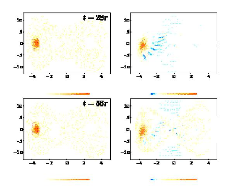
FIG. 10.: Classical (left) and quantum (right) evolution of the Gaussian state initially localized at the leftmost regular island (see Section 2A) when the system is opened to the action of the environment environment ($D=0.01$), for the tunneling case.

FIG. 11.: Time series of the quantum expectation value of $x$ for the state of Fig.3

It is interesting to notice that this picture would drastically change if the coupling to the environment is switched on at a time $t_{0}>0$ (i.e., if we let the system to evolve freely, with its own Hamiltonian, before coupling it to the environment). This is very easy to do using the above master equation. The results obtained in this way are simple and intuitive: If we switch on the coupling to the environment at a time when the system has already tunneled to the pair related island on the right ($t=56\tau$), the environment will simply stop the state from tunnelling back to the initial island. Figure 12 (right) shows the evolution of the Wigner function in this case. Contrariwise, if we turn on the coupling to the environment when the state is half way through the tunnelling (in an intermediate, delocalized, state at time $t_{0}=28\tau$), decoherence yields an asymptotic state which has approximately half of the probability in each side of the well (this is seen on the left column of Figure 12).

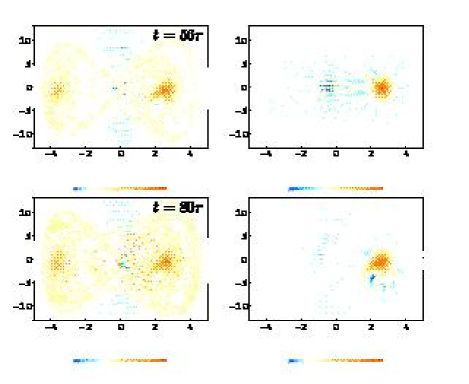
FIG. 12.: Evolution of the Gaussian state initially localized at the leftmost regular island (see Section 2A) when the environment ($D=0.01$) is connected at $t_{0}=28\tau$ (on the left) or at $t_{0}=56\tau$ (on the right).

VI conclusion

Quantum open systems become entangled with the environments as a consequence of their interaction. For this reason, information initially stored in the state of the system irreversibly leaks into the environment. The results we presented here support the point of view stating [14] that for classically chaotic systems the rate at which information flows from the system to the environment (the rate of von Neuman entropy production) is independent of the strength of the coupling to the environment (provided the coupling strength is above some threshold). Thus, our results show that for chaotic quantum systems, the classical limit enforced by environment induced decoherence is quite different from the one corresponding to regular systems. Thus, we showed that this limit exhibits an unavoidable source of unpredictability, being the rate at which information is lost into the environment entirely fixed by the chaotic nature of the Hamiltonian of the system. To the contrary, for regular systems the entropy production rate is proportional to the strength of the coupling to the environment. Therefore, the existence of this phase of coupling–independent entropy production could be used as a diagnostic for quantum chaos. Our results also confirm previous estimations [14, 17] for the transition time $t_{c}$ between the two regimes: the one where the entropy production rate is diffusion-dominated and the one set by the chaotic dynamics, that is, a linear dependence of $t_{c}$ on the initial entropy (initial spread) and a logarithmic dependence on the diffusion constant.

From our results it is possible to develop an intuitive picture for the reason why entropy production rate becomes dominated by the chaotic dynamic. As we described in the paper, there are two interrelated processes contributing to the growth of entropy. First, the destruction of the interference fringes which are dynamically produced in phase space by the streaching and folding of the chaotic evolution. The entropy production rate associated with this process is obviously determined by the slowest of the two timescales corresponding to the proceses of creation and anihillation of fringes. Therefore, when decoherence is effective, and the fringes dissappear in a short timescale, the entropy production rate is of dynamical origin (and independent of the coupling strength between the system and the environment). On the other hand the spread of the possitive peaks of the Wigner function also contributes to the entropy growth. In this case, the rate becomes independent of the coupling strength once the phase space distribution approaches a critical width. Both of these processes are present in a general case (only it is possible to study them separately in idealized cases such as in the baker’s map [46]). The results of this paper confirm this intuitive view, which can be made more precise when formulated in terms of equation (13).

This work was partially supported by Ubacyt (TW23), Anpcyt, Conicet and Fundación Antorchas. JPP thanks W. Zurek for many useful discussions and hospitality during his visits to Los Alamos.

REFERENCES

- [1] Zurek, W. H., Physics Today 44, 36 (1991).
- [2] Giulini, D., Joos, E., Kiefer, C., Kupsch, J., Stamatescu, I.-O., and Zeh, H. D., Decoherence and the Appearance of a Classical World in Quantum Theory, (Springer, Berlin, 1996).
- [3] Zurek, W. H., Phys. Rev. D 24, 1516-1524 (1981).
- [4] Zurek, W. H., Phys. Rev. D 26, 1862-1880 (1982).
- [5] Zurek, W. H., pp. 145-149 in Frontiers of Non-equilibrium Statistical Mechanics, G. T. Moore and M. O. Scully, eds. (Plenum, New York, 1986).
- [6] Paz, J. P., Habib, S., and Zurek, W. H., Phys. Rev. D 47, 488 (1993).
- [7] Zurek, W. H., Progr. Theor. Phys. 89, 281-302 (1993).
- [8] Zurek, W. H., Habib, S., and Paz, J. P., Phys. Rev. Lett., 70, 1187, (1993).
- [9] Paz, J. P. and Zurek, W. H., Phys. Rev. Lett. 82, 5181 (1999).
- [10] Paz, J. P. and Zurek, W. H., quant-ph/0010011, to appear in the “Proceedings of the 72nd. Les Houches Summer School”, Springer Verlag (2001), in press.
- [11] Brune, M., Hagley, E., Dreyer, J., Maître, X., Maali, A., Wunderlich, C., Raimond, J-M., and Haroche, S., Phys. Rev. Lett. 77, 4887-4890 (1996).
- [12] Cheng, C. C., and Raymer, M. G., Phys. Rev. Lett, 82, 4802 (1999)
- [13] Myatt, C. J., et al., Nature, 403, 269 (2000).
- [14] Zurek, W. H., and Paz, J. P., Phys. Rev. Lett. 72, 2508-2511 (1994); ibid. 75, 351 (1995).
- [15] Zurek, W. H. and Paz, J. P., Physica D83, 300 (1995).
- [16] Habib, S., Shizume, K., and Zurek, W. H., Phys. Rev. Lett, 80, 4361 (1998).
- [17] Monteoliva, D., and Paz, J. P., Phys. Rev. Lett. 87 (2000) 3373.
- [18] Wisdom, J., Peale, S. J., and Maignard, F. Icarus 58, 137 (1984); see also Wisdom, J., Icarus 63, 272 (1985); Laskar, J., Nature 338, 237 (1989); Sussman, G. J., and Wisdom, J., Science 257, 56-62 (1992).
- [19] Wigner, E. P., Phys. Rev. 40, 749 (1932). For a review, see Hillery, M., O’Connell, R. F., Scully, M. O., and Wigner, E. P., Phys. Rep. 106, 121 (1984).
- [20] Zurek, W. H., Physica Scripta T76, 186 (1998), also available at quant-ph/9802054.
- [21] Karkuszewski Z., Zakrezewski J. and Zurek, W. H. Breakdown of correspondence in chaotic systems: Ehrenfest versus localization times, preprint available at nlin.CD/0012048.
- [22] Hu, B. L., Paz, J. P., and Zhang, Y., Phys. Rev. D 45, 2843 (1992).
- [23] Caldeira, A. O., and Leggett, A. J., Physica 121A, 587-616 (1983); Phys. Rev. A 31, 1059 (1985).
- [24] Unruh, W. G., and Zurek, W. H., Phys. Rev. D 40, 1071-1094 (1989).
- [25] Shiokawa, K., and Hu, B. L., Phys. Rev E 52, 2497 (1995).
- [26] Miller, P. A., and Sarkar, S. Phys. Rev. E 58, 4217 (1998); E 60, 1542 (1999).
- [27] Jalabert R. and Pastawski, H., Phys. Rev. Lett. 86, 2490 (2001) and references therein.
- [28] Pattanayak, A. K., Phys. Rev. Lett. 83, 4526 (2000).
- [29] Graham R., Z. Phys. B59, 75 (1985); Graham R. and Tel T., Z. Phys. B60, 127 (1985); Dittrich T. and Graham R., Z. Phys. B62, 515 (1986).
- [30] F. Haake, Quantum signatures of chaos, Springer Series in Synergetics, edited by H. Haken, vol 54, Springer (Berlin, 1991).
- [31] Dittrich T., Hänggi P., Ingold G.-L., Kramer B., Shön G. and Zwerger W., Quantum transport and dissipation, Wiley–VCH (1998).
- [32] L. E. Reichl and W. Zheng, Phys. Rev. A 29 (1984) 2186.
- [33] W. A. Lin and L. E. Ballentine, Phys. Rev. A 45 (1992) 3637; Phys. Rev. Lett 65 (1990) 2927.
- [34] M. Feit J. Fleck Jr. and A. Steiger, J. Comp. Phys. 47 (1992) 412.
- [35] J. Shirley, Phys. Rev. A 138 B (1965) 979.
- [36] K. F. Milfeld and R. Wyatt, Phys. Rev. A 27 (1983) 72.
- [37] K Takahashi, Prog. Theor. Phys. Supp. bf 98 (1989) 109.
- [38] M. Berry and N. L. Balazs, J. Phys. A 12 (1979) 625.
- [39] R. Utermann, T. Dittrich and P. Hánggi, Phys. Rev. E 49 (1994) 273.
- [40] F. Grossmann, T. Dittrich, P. Jung and P. Hánggi, J. Stat. Phys. 70 (1993) 229.
- [41] T. Dittrich, B. Oelschlägel and P. Hánggi, Europhys. Lett. 22 (1993) 5.
- [42] R.Blümel, A.Buchleitner, R. Graham, L. Sirko, U. Smilansky and H. Walther, Phys. Rev. A44 (1991) 4521.
- [43] Zurek, W. H. (2000) private communication.
- [44] P. Hänggi, S. Kohler and T. Dittrich, in Proc. 1999 LNP 547, edited by D. Regera et al; (1999) 125–157, Springer Verlag (Berlin); S. Kohler, R. Utermann, P. Hänggi and T. Dittich, Phys. Rev. E58 (1998) 7219 (also quant-ph/9804041).
- [45] S. Habib and R. Ryne, Phys. Rev. Lett 74 (1995) 70.
- [46] P. Bianucci, J.P. Paz and M. Saraceno, Decoherence for classically chaotic quantum maps, (2001) to be published.