Entanglement-Assisted Capacity of a Quantum Channel and the Reverse Shannon Theorem

Abstract

The entanglement-assisted classical capacity of a noisy quantum channel ($C_{E}$) is the amount of information per channel use that can be sent over the channel in the limit of many uses of the channel, assuming that the sender and receiver have access to the resource of shared quantum entanglement, which may be used up by the communication protocol. We show that the capacity $C_{E}$ is given by an expression parallel to that for the capacity of a purely classical channel: i.e., the maximum, over channel inputs $\rho$, of the entropy of the channel input plus the entropy of the channel output minus their joint entropy, the latter being defined as the entropy of an entangled purification of $\rho$ after half of it has passed through the channel. We calculate entanglement-assisted capacities for two interesting quantum channels, the qubit amplitude damping channel and the bosonic channel with amplification/attenuation and Gaussian noise. We discuss how many independent parameters are required to completely characterize the asymptotic behavior of a general quantum channel, alone or in the presence of ancillary resources such as prior entanglement. In the classical analog of entanglement assisted communication—communication over a discrete memoryless channel (DMC) between parties who share prior random information—we show that one parameter is sufficient, i.e., that in the presence of prior shared random information, all DMC’s of equal capacity can simulate one another with unit asymptotic efficiency.

I. Introduction

The formula for the capacity of a classical channel was derived in 1948 by Shannon. It has long been known that this formula is not directly applicable to channels with significant quantum effects. Extending this theorem to take quantum effects into account has been harder than might have been anticipated; despite much recent effort, we do not yet have a comprehensive theory for the capacity of quantum channels. The book of Nielsen and Chuang [28] and the survey paper [8] are two sources giving good overviews of quantum information theory. In this paper, we advance quantum information theory by proving a capacity formula for quantum channels which holds when the sender and receiver have access to shared quantum entangled states which can be used in the communication protocol. We also present a conjecture that would imply that, in the presence of shared entanglement, to first order this entanglement-assisted capacity is the only quantity determining the asymptotic behavior of a quantum channel.

A (memoryless) quantum communications channel can be viewed physically as a process wherein a quantum system interacts with an environment (which may be taken to initially be in a standard state) on its way from a sender to a receiver; it may be defined mathematically as a completely positive, trace-preserving linear map on density operators. The theory of quantum channels is richer and less well understood than that of classical channels. For example, quantum channels have several distinct capacities, depending on what one is trying to use them for, and what additional resources are brought into play. These include

• The ordinary classical capacity $C$, defined as the maximum asymptotic rate at which classical bits can be transmitted reliably through the channel, with the help of a quantum encoder and decoder.

• The ordinary quantum capacity $Q$, which is the maximum asymptotic rate at which qubits can be transmitted under similar circumstances.

• The classically assisted quantum capacity $Q_{2}$, which is the maximum asymptotic rate of reliable qubit transmission with the help of unlimited use of a 2-way classical side channel between sender and receiver.

• The entanglement assisted classical capacity $C_{E}$, which is the maximum asymptotic rate of reliable bit transmission with the help of unlimited prior entanglement between the sender and receiver.

Somewhat unexpectedly, the last of these has turned out to be the simplest to calculate, because, as we show in section II, it is given by an expression analogous to the formula expressing the classical capacity of a classical channel as the maximum, over input distributions, of the input:output mutual information. Section III calculates entanglement assisted capacities of the amplitude damping channel and of amplifying and attenuating bosonic channels with Gaussian noise.

We return now to a general discussion of quantum channels and capacities, in order to provide motivation for section IV of the paper, on what we call the reverse Shannon theorem.

Aside from the constraints $Q\!\leq\!C\!\leq\!C_{E}$, and $Q\!\leq\!Q_{2}$, which are obvious consequences of the definitions, the four capacities appear to vary rather independently. It is conjectured that $Q_{2}\!\leq\!C$, but this has not been proved to date. Except in special cases, it is not possible, without knowing the parameters of a channel, to infer any one of its four capacities from the other three. This independence is illustrated in Table 1, which compares the capacities of several simple channels for which they are known exactly. The channels incidentally illustrate four different degrees of qualitative quantumness: the first can carry qubits unassisted, the second requires classical assistance to do so, the third has no quantum capacity at all but still exhibits quantum behavior in that its capacity is increased by entanglement, while the fourth is completely classical, and so unaffected by entanglement.

Table 1: Capacities of several quantum channels.

Channel	$Q$	$Q_{2}$	$C$	$C_{E}$
Noiseless qubit channel	1	1	1	2
50% erasure qubit channel	0	1/2	1/2	1
2/3 depolarizing qubit channel	0	0	0.0817∗	0.2075
Noiseless bit channel =	0	0	1	1
100% dephasing qubit channel

^∗Proved in [24].

Contrary to an earlier conjecture of ours, we have found channels for which $Q\!>\!0$ but $C\!=\!C_{E}$. One example is a channel mapping three qubits to two qubits which is switched between two different behaviors by the first input qubit. The channel operates as follows: The first qubit is measured in the ${|0\rangle},\,{|1\rangle}$ basis. If the result is ${|0\rangle}$, then the other two qubits are dephased (i.e., measured in the ${|0\rangle}$, ${|1\rangle}$ basis) and transmitted as classical bits; if the result is ${|1\rangle}$, the first qubit is transmitted intact and the second qubit is replaced by the completely mixed state. This channel has $Q\!=\!Q_{2}\!=\!1$ (achieved by setting the first qubit to ${|1\rangle}$) and $C\!=\!C_{E}\!=\!2$.

This complex situation naturally raises the question of how many independent parameters are needed to characterize the important asymptotic, capacity-like properties of a general quantum channel. A full understanding of quantum channels would enable us to calculate not only their capacities, but more generally, for any two channels ${\cal M}$ and ${\cal N}$, the asymptotic efficiency (possibly zero) with which ${\cal M}$ can simulate ${\cal N}$, both alone and in the presence of ancillary resources such as classical communication or shared entanglement.

One motivation for studying communication in the presence of ancillary resources is that it can simplify the classification of channels’ capacities to simulate one another. This is so because if a simulation is possible without the ancillary resource, then the simulation remains possible with it, though not necessarily vice versa. For example, $Q$ and $C$ represent a channel’s asymptotic efficiencies of simulating, respectively, a noiseless qubit channel and a noiseless classical bit channel. In the absence of ancillary resources these two capacities can vary independently, subject to the constraint $Q\leq C$, but in the presence of unlimited prior shared entanglement, the relation between them becomes fixed: $C_{E}=2Q_{E}$, because shared entanglement allows a noiseless 2-bit classical channel to simulate a noiseless 1-qubit channel and vice versa (via teleportation [6] and superdense coding [9]).

We conjecture that prior entanglement so simplifies the complex landscape of quantum channels that only a single free parameter remains. Specifically, we conjecture that in the presence of unlimited prior entanglement, any two quantum channels of equal $C_{E}$ could simulate one another with unit asymptotic efficiency. Section IV proves a classical analog of this conjecture, namely that in the presence of prior random information shared between sender and receiver, any two discrete memoryless classical channels (DMC’s) of equal capacity can simulate one another with unit asymptotic efficiency. We call this the classical reverse Shannon theorem because it establishes the ability of a noiseless classical DMC to simulate noisy ones of equal capacity, whereas the ordinary Shannon theorem establishes that noisy DMC’s can simulate noiseless ones of equal capacity.

Another ancillary resource—classical communication—also simplifies the landscape of quantum channels, but probably not so much. The presence of unlimited classical communication does allow certain otherwise inequivalent pairs of channels to simulate one another (for example, a noiseless qubit channel and a 50% erasure channel on 4-dimensional Hilbert space), but it does not render all channels of equal $Q_{2}$ asymptotically equivalent. So-called bound-entangled channels [21, 15] have $Q_{2}\!=\!0$, but unlike classical channels (which also have $Q_{2}\!=\!0$) they can be used to prepare bound entangled states, which are entangled but cannot be used to prepare any pure entangled states. Because the distinction between bound entangled and unentangled states does not vanish asymptotically, even in the presence of unlimited classical communication [32], bound-entangled and classical channels must be asymptotically inequivalent, despite having the same $Q_{2}$.

The various capacities of a quantum channel ${\cal N}$ may be defined within a common framework,

$$C_{X}({\cal N})=\lim_{\epsilon\rightarrow 0}\limsup_{n\rightarrow\infty}\;\{\frac{m}{n}:\exists_{{\cal A}}\exists_{{\cal B}}\forall_{\psi\in\Gamma_{m}}\;F(\psi,{\cal A},{\cal B},{\cal N})\;>1\!-\!\epsilon\;\;\}.$$ (1)

Here $C_{X}$ is a generalized capacity; ${\cal A}$ is an encoding subprotocol, to be performed by Alice, which receives an $m$-qubit state $\psi$ belonging to some set $\Gamma_{m}$ of allowable inputs to the entire protocol, and produces $n$ possibly entangled inputs to the channel ${\cal N}$; ${\cal B}$ is a decoding subprotocol, to be performed by Bob, which receives $n$ (possibly entangled) channel outputs and produces an $m$-qubit output for the entire protocol; finally $F(\psi,{\cal A},{\cal B},{\cal N})$ is the fidelity of this output relative to the input $\psi$, i.e., the probability that the output state would pass a test determining whether it is equal to the input (more generally, the fidelity of one mixed state $\rho$ relative to another $\sigma$ is $F=({\rm tr}(\sqrt{\rho}\;\sigma\sqrt{\rho}))^{2}$). Different capacities are defined depending on the specification of $\Gamma$, ${\cal A}$ and ${\cal B}$. The classical capacities $C$ and $C_{E}$ are defined by restricting $\psi$ to a standard orthonormal set of states, without loss of generality the “Boolean” states labelled by bit strings $\Gamma_{m}=\{{|0\rangle},{|1\rangle}\}^{\otimes m}$; for the quantum capacities $Q$ and $Q_{2}$, $\Gamma_{m}$ is the entire $2^{m}$ dimensional Hilbert space ${\cal H}_{2}^{\otimes m}$. For the simple capacities $Q$ and $C$, the Alice and Bob subprotocols are completely-positive trace-preserving maps from ${\cal H}_{2}^{\otimes m}$ to the input space of ${\cal N}^{\otimes n}$, and from the output space of ${\cal N}^{\otimes n}$ back to ${\cal H}_{2}^{\otimes m}$. For $C_{E}$ and $Q_{2}$, the subprotocols are more complicated, in the first case drawing on a supply of ebits (maximally entangled pairs of qubits) shared beforehand between Alice and Bob, and in the latter case making use of a 2-way classical channel between Alice and Bob. The definition of $Q_{2}$ thus includes interactive protocols, in which the $n$ channel uses do not take place all at once, but may be interspersed with rounds of classical communication.

The classical capacity of a classical discrete memoryless channel is also given by an expression of the same form, with $\psi$ restricted to Boolean values; the encoder ${\cal A}$, decoder ${\cal B}$, and channel ${\cal N}$ all being restricted to be classical stochastic maps; and the fidelity $F$ being defined as the probability that the (Boolean) output of ${\cal B}({\cal N}^{\otimes n}({\cal A}(\psi)))$ is equal to the input $\psi$. We will sometimes indicate these restrictions implicitly by using upper case italic letters (e.g. $N$) for classical stochastic maps, and lower case italic letters (e.g. $x$) for classical discrete data. The definition of classical capacity would then be

$$C(N)=\lim_{\epsilon\rightarrow 0}\limsup_{n\rightarrow\infty}\;\{\frac{m}{n}:\exists_{A}\exists_{B}\;\forall_{x\in\{0,1\}^{m}}F(x,A,B,N)\;>1\!-\!\epsilon\;\;\}.$$ (2)

A classical stochastic map, or classical channel, may be defined in quantum terms as one that is completely dephasing in the Boolean basis both with regard to its inputs and its outputs. A channel, in other words, is classical if and only if it can be represented as a composition

$$N={\cal D^{\prime}GD}$$ (3)

of the completely dephasing channel ${\cal D}$ on the input Hilbert space, followed by a general quantum channel ${\cal G}$, followed by the completely dephasing channel ${\cal D^{\prime}}$ on the output Hilbert space (a completely dephasing channel is one that makes a von Neumann measurement in the Boolean basis and resends the result of the measurement). Dephasing only the inputs, or only the outputs, is in general insufficient to abolish all quantum properties of a quantum channel ${\cal G}$.

The notion of capacity may be further generalized to define a capacity of one channel ${\cal N}$ to simulate another channel ${\cal M}$. This may be defined as

$$C_{X}({\cal N,M})=\lim_{\epsilon\rightarrow 0}\limsup_{n\rightarrow\infty}\{\frac{m}{n}:\exists_{\cal A,B}\forall_{\psi\in H_{M}^{\otimes m}}\;F({\cal M}^{\otimes m}(\psi),{\cal A},{\cal B},{\cal N})\;>1\!-\!\epsilon\;\;\},$$ (4)

where ${\cal A}$ and ${\cal B}$ are respectively Alice’s and Bob’s subprotocols which together enable Alice to receive an input $\psi$ in $H_{M}^{\otimes m}$ (the tensor product of $m$ copies of the input Hilbert space $H_{M}$ of the channel ${\cal M}$ to be simulated) and, making $n$ forward uses of the simulating channel ${\cal N}$, allow Bob to produce some output state, and $F({\cal M}^{\otimes m}(\psi),{\cal A},{\cal B},{\cal N})$ is the fidelity of this output state with respect to the state that would have been generated by sending the input $\psi$ through ${\cal M}^{\otimes m}$.

These definitions of capacity are all asymptotic, depending on the properties of ${\cal N}^{\otimes n}$ in the limit $n\!\rightarrow\!\infty$. However, several of the capacities are given by, or closely related to, non-asymptotic expressions involving input and output entropies for a single use of the channel. Figure 1 shows a scenario in which a quantum system $Q$, initially in mixed state $\rho$, is sent through the channel, emerging in a mixed state ${\cal N}(\rho)$. It is useful to think of the initial mixed state as being part of an entangled pure state $\Phi_{\rho}^{QR}$ where $R$ is some reference system that is never operated upon physically. Similarly the channel can be thought of as a unitary interaction $U$ between the quantum system $Q$ and some environment subsystem $E$, which is initially supplied in a standard pure state $0^{E}$, and leaves the interaction in a mixed state ${\cal E}(\rho)^{E}$. Thus ${\cal N}$ and ${\cal E}$ are completely positive maps relating the final states of the channel output and environment, respectively, to the initial state of the channel input, when the initial state of the environment is held fixed. The mnemonic superscripts $Q,R,E$ indicate, when necessary, to what system a density operator refers.

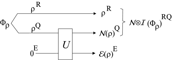
Figure 1: A quantum system Q in mixed state $\rho$ is sent through the noisy channel ${\cal N}$, which may be viewed as a unitary interaction $U$ with an environment E. Meanwhile a purifying reference system R is sent through the identity channel ${\cal I}$. The final joint state of RQ has the same entropy as the final state ${\cal E}(\rho)$ of the environment.

Under these circumstances three useful von Neumann entropies may be defined, the input entropy

$$H(\rho^{Q})=-{\rm tr}\rho^{Q}\log_{2}\rho^{Q},$$

the output entropy

$$H({\cal N}(\rho)^{Q}),$$

and the entropy exchange

$$H(({\cal N}\otimes{\cal I})\Phi_{\rho}^{QR})=H({\cal E}(\rho)^{E}).$$

The complicated left side of the last equation represents the entropy of the joint state of the subsystem $Q$ which has been through the channel, and the reference system $R$, which has not, but may still be more or less entangled with it. The density operator $({\cal N}\otimes{\cal I})\Phi_{\rho}$ is the quantum analog of a joint input:output probability distribution, because it has ${\cal N}(\rho)$ and $\rho$ as its partial traces. Without the reference system, the notion of a joint input:output mixed state would be problematic, because the input and output are not present at the same time, and the no-cloning theorem prevents Alice from retaining a spare copy of the input to be compared with the one sent through the channel. The entropy exchange is also equal to the final entropy of the environment $H({\cal E}(\rho))$, because the tripartite system $QRE$ remains throughout in a pure state; making its two complementary subsystems $E$ and $QR$ always isospectral. The relations between these entropies and quantum channels have been well reviewed by Schumacher and Nielsen  [30] and by Holevo and Werner [18].

By Shannon’s theorem, the capacity of a classical channel $N$ is the maximum, over input distributions, of the input:output mutual information, in other words the input entropy plus the output entropy less the joint entropy of input and output. The quantum generalization of mutual information for a bipartite mixed state $\rho^{AB}$, which reduces to classical mutual information when $\rho^{AB}$ is diagonal in a product basis of the two subsystems, is

$$H(\rho^{A})+H(\rho^{B})-H(\rho^{AB}).$$

where

$$\rho^{A}\!={\rm tr}_{B}\rho^{AB}\qquad\hbox{and}\qquad\rho^{B}\!={\rm tr}_{A}\rho^{AB}.$$

In terms of Figure 1, the classical capacity of a classical channel (cf. eq. (3)) can be expressed as

$$C(N)=\max_{\rho\in\Delta}H(\rho)+H(N(\rho))-H((N\otimes{\cal I})(\Phi_{\rho}))$$ (5)

where $\Delta$ is the class of density operators on the channel’s input Hilbert space that are diagonal in the Boolean basis. The third term (entropy exchange), for a classical channel $N$, is just the joint Shannon entropy of the classically correlated Boolean input and output, because the von Neumann entropies reduce to Shannon entropies when evaluated in the Schmidt basis of $\Phi_{\rho}$, with respect to which all states are diagonal. The restriction to classical inputs $\rho\in\Delta$ can be removed, because any non-diagonal elements in $\rho$ would only reduce the first term, while leaving the other two terms unchanged, by virtue of the diagonality-enforcing properties of the channel.

Thus, the expression

$$\max_{\rho\in{\cal H}_{\rm{in}}}H(\rho)+H({\cal N}(\rho))-H(({\cal N}\otimes{\cal I})\Phi_{\rho}),$$ (6)

is a natural generalization to quantum channels ${\cal N}$ of a classical channel’s maximal input:output mutual information, and it is equal to the classical capacity whenever ${\cal N}$ is classical, as defined previously in this section.

One might hope that this expression continues to give the classical capacity of a general quantum channel ${\cal N}$, but that is not so, as can be seen by considering the simple case ${\cal N=I}$ of a noiseless qubit channel. Here the maximum is attained on a uniform input mixed state $\rho=I/2$, causing the first two terms each to have the value 1 bit, while the last term is zero, giving a total of 2 bits. This is not the ordinary classical capacity of the noiseless qubit channel, which is equal to 1 bit, but rather its entanglement-assisted capacity $C_{E}({\cal N})$. In the next section we show that this is true of quantum channels in general, as stated by the following theorem.

Theorem 1

Given a quantum channel ${\cal N}$, then the entanglement-assisted capacity of the quantum channel $C_{E}$ is equal to the maximal quantum mutual information

$$C_{E}=\max_{\rho\in{\cal H}_{\rm{in}}}H(\rho)+H({\cal N}(\rho))-H(({\cal N}\otimes{\cal I})\Phi_{\rho}).$$ (7)

Here the capacity $C_{E}$ is defined as the supremum of Eq. (1) when $\psi$ ranges over Boolean states and ${\cal A}$, ${\cal B}$ over all protocols where Alice and Bob start with an arbitrarily large number of shared EPR pairs, but have no access to any communication channels other than ${\cal N}$.

Another capacity theorem which has been proven for quantum channels is the Holevo-Schumacher-Westmoreland theorem [19, 31], which says that if the signals that Bob receives are constrained to lie in a set of quantum states $\rho^{\prime}_{i}$, where Alice chooses $i$ (for example, by supplying input state $\rho_{i}$ to the channel ${\cal N}$) then the capacity is given by

$$C_{H}(\{\rho^{\prime}_{i}\})=H(\sum_{i}p_{i}\rho^{\prime}_{i})-\sum_{i}p_{i}H(\rho^{\prime}_{i}).$$ (8)

This gives a means to calculate a constrained classical capacity for a quantum channel ${\cal N}$ if the sender is not allowed to use entangled inputs: the channel’s Holevo capacity $C_{H}({\cal N})$ being defined as the maximum of $C_{H}(\{{\cal N}(\rho_{i})\})$ over all possible sets of input states $\{\rho_{i}\}$. We will be using this theorem extensively in the proof of our entanglement-assisted capacity bound.

In our original paper [7], we proved the formula (6) for certain special cases, including the depolarizing channel and the erasure channel. We did this by sandwiching the entanglement-assisted capacity between two other capacities, which for certain channels turned out to be equal. The higher of these two capacities we called the forward classical communication cost via teleportation, ($FCCC_{Tp}$), which is the amount of forward classical communication needed to simulate the channel ${\cal N}$ by teleporting over a noisy classical channel. The lower of these two bounds we called $C_{Sd}$, which is the capacity obtained by using the noisy quantum channel ${\cal N}$ in the superdense coding protocol. We have that $C_{Sd}\leq C_{E}\leq FCCC_{Tp}$. Thus, if $C_{Sd}=FCCC_{Tp}$ for a channel, we have obtained the entanglement-assisted capacity of the channel. In order for this argument to work, we needed the classical reverse Shannon theorem, which says that a noisy classical channel can be simulated by a noiseless classical channel of the same capacity, as long as the sender and receiver have access to shared random bits. We needed this theorem because the causality argument showing that EPR pairs do not add to the capacity of a classical channel appears to work only for noiseless channels. We sketched the proof of the classical reverse Shannon theorem in our previous paper, and give it in full in this paper.

In our previous paper, the bounds $C_{Sd}$ and $FCCC_{Tp}$ are both computed using single-symbol protocols; that is, both the superdense coding protocol and the simulation of the channel by teleportation via a noisy classical channel are carried out with a single use of the channel. The capacity is then obtained using the classical Shannon formula for a classical channel associated with these protocols. In this paper, we obtain bounds using multiple-symbol protocols, which perform entangled operations on many uses of the channel. We then perform the capacity computations using the Holevo-Schumacher-Westmoreland formula (8).

II. Formula for Entanglement Assisted Classical Capacity

Assume we have a quantum channel ${\cal N}$ which maps a Hilbert space ${\cal H}_{\rm{in}}$ to another Hilbert space ${\cal H}_{\rm{out}}$. Let $C_{E}$ be the classical capacity of the channel when the sender and receiver have an unbounded supply of EPR pairs to use in the communication protocol. This section proves that the entanglement-assisted capacity of a channel is the maximum quantum mutual information attainable between the two parts of an entangled quantum state, one part of which has been passed through the channel. That is,

$$C_{E}({\cal N})=\max_{\rho\in{\cal H}_{\rm{in}}}\ \ H(\rho)+H({\cal N}(\rho))-H(({\cal N}\otimes{\cal I})\Phi_{\rho}),$$ (9)

where $H(\rho)$ denotes the von Neumann entropy of a density matrix $\rho\in{\cal H}_{\mathrm{in}}$, $H({\cal N}(\rho))$ denotes the von Neumann entropy of the output when $\rho$ is input into the channel, and $H(({\cal N}\otimes{\cal I})\Phi_{\rho})$ denotes the von Neumann entropy of a purification $\Phi_{\rho}$ of $\rho$ over a reference system ${\cal H}_{\mathrm{ref}}$, half of which (${\cal H}_{\mathrm{in}}$) has been sent through the channel ${\cal N}$ while the other half (${\cal H}_{\mathrm{ref}}$) has been sent through the identity channel ${\cal I}$ (this corresponds to the portion of the entangled state that Bob holds at the start of the protocol). Here, we have $\Phi_{\rho}\in{\cal H}_{\rm{in}}\otimes{\cal H}_{\rm{ref}}$ and ${\rm Tr}_{\rm{ref}}\Phi_{\rho}=\rho$. All purifications of $\rho$ give the same entropy in this formula, so we need not specify which one we use. As pointed out earlier, the right hand side of Eq. (9) parallels the expression for capacity of a classical channel as the maximum, over input distributions, of the input:output mutual information.

Lindblad [26], Barnum et al. [3], and Adami and Cerf [12] characterized several important properties of the quantum mutual information, including positivity, additivity and the data processing inequality. Adami and Cerf argued that the right side of Eq. (9) represents an important channel property, calling it the channel’s “von Neumann capacity”, but they did not indicate what kind of communication task this capacity represented the channel’s asymptotic efficiency for doing. Now we know that it is the channel’s efficiency for transmitting classical information when the sender and receiver share prior entanglement.

In our demonstration that Eq. (9) is indeed the correct expression for entanglement assisted classical capacity, the first subsection gives an entanglement assisted classical communication protocol which can asymptotically achieve the rate ${\mathrm{RHS}}-\epsilon$ for any $\epsilon$. The second subsection gives a proof of a crucial lemma on typical subspaces needed in the first subsection. The third subsection shows that the right hand side of Eq. (9) is indeed an upper bound for $C_{E}({\cal N})$. The fourth subsection proves several entropy inequalities that are used in the third subsection.

A. Proof of the Lower Bound

In this section, we will prove the inequality

$$C_{E}({\cal N})\geq\max_{\rho\in{\cal H}_{\rm{in}}}\ \ H(\rho)+H({\cal N}(\rho))-H({\cal N}\!\!\otimes\!{\cal I}\;(\Phi_{\rho})).$$ (10)

We first show the inequality

$$C_{E}({\cal N})\geq H(\rho)+H({\cal N}(\rho))-H({\cal N}\!\!\otimes\!{\cal I}\;(\Phi_{\rho}))$$ (11)

for the special case where $\rho=\frac{1}{d}I$, where $d=\dim{\cal H}_{\rm{in}}$, $I$ is the identity matrix, and $\Phi_{\rho}$ is a maximally entangled state. We then use this special case to show that the inequality (11) still holds when $\rho$ is any projection matrix. We finally use the case where $\rho$ is a projection matrix to prove the inequality in the general case of arbitrary $\rho$, showing (10); we do this by taking $\rho^{\prime}$ to be the projection onto the typical subspace of $\rho^{\otimes n}$, and using $\rho^{\prime}$ and ${\cal N}^{\otimes n}$ in the inequality (11).

The coding protocol we use for the special case given above, where $\rho=\frac{1}{d}I$, is essentially the same as the protocol used for quantum superdense coding [9], which procedure yields the entanglement-assisted capacity in the case of a noiseless quantum channel. The proof that the formula (11) holds for $\rho=I/d$, however, is quite different from and somewhat more complicated than the proof that superdense coding works. Our proof uses Holevo’s formula (8) for quantum capacity to compute the capacity achieved by our protocol. This protocol is the same as that given in our earlier paper on $C_{E}$ [7], although our proof is different; the earlier proof only applied to certain quantum channels, such as those that commute with teleportation.

We need to use the generalization of the Pauli matrices to $d$ dimensions. These are the matrices used in the $d$-dimensional quantum teleportation scheme [6]. There are $d^{2}$ of these matrices, which are given by $U_{j,k}=T^{j}R^{k}$, for the matrices $T$ and $R$ defined by their entries as

$$T_{a,b}=\delta_{a,\,b-1{\rm{\,mod\,}}d}{\rm{\ \ and\ \ }}R_{a,b}=e^{2\pi ia/d}\delta_{a,b}$$ (12)

as in [2]. To achieve the capacity given by the above formula (11) with $\rho=I/d$, Alice and Bob start by sharing a $d$-dimensional maximally entangled state $\phi$. Alice applies one of the $d^{2}$ transformations $U_{j,k}$ to her part of $\phi$, and then sends it through the channel ${\cal N}$. Bob gets one of the $d^{2}$ quantum states $({\cal N}\otimes{\cal I})(U_{j,k}\otimes{\cal I})\phi$. It is straightforward to show that averaging over the matrices $U_{j,k}$ effectively disentangles Alice’s and Bob’s pieces, so we obtain

$$\sum_{j,k=1}^{d}({\cal N}\otimes{\cal I})(U_{j,k}\otimes{\cal I})\phi = {\cal N}({\rm Tr}_{B}\phi)\otimes{\rm Tr}_{A}\phi$$ (13)

$$= {\cal N}(\rho)\otimes\rho$$

where $\rho=\frac{1}{d}I$. The entropy of this quantity is the first term of Holevo’s formula 8, and gives the first two terms of (11). The entropy of each of the $d^{2}$ states $({\cal N}\otimes{\cal I})(U_{j,k}\otimes{\cal I})\phi$ is $H(({\cal N}\otimes{\cal I})(\Phi_{\rho}))$, since each of the $(U_{j,k}\otimes{\cal I})(\phi)$ is a purification of $\rho$. This entropy is the second term of Holevo’s formula 8, and gives the third term of (11). We thus obtain the formula when $\rho=\frac{1}{d}I$.

The next step is to note that the inequality (11) also holds if the density matrix $\rho$ is a projection onto any subspace of ${\cal H}_{\rm{in}}$. The proof is exactly the same as for $\rho=\frac{1}{d}I$. In fact, one can prove this case by using the above result. By restricting ${\cal H}_{\rm{in}}$ to the support of $\rho$, which we can denote by ${\cal H}^{\prime}$, and by restricting ${\cal N}$ to act only on ${\cal H}^{\prime}$, we obtain a channel ${\cal N}^{\prime}$ for which $\rho^{\prime}=\frac{1}{d_{\mathrm{in}}^{\prime}}I$.

We now must show that (11) holds for arbitrary $\rho$. This is the most difficult part of the proof. For this step we need a little more notation. Recall that we can assume that any quantum map ${\cal N}$ can be implemented via a unitary transformation ${\cal U}$ acting on the system ${\cal H}_{\rm{in}}$ and some environment system ${\cal H}_{\rm{env}}$, where ${\cal H}_{\rm{env}}$ starts in some fixed initial state. We introduce ${\cal E}$, which is the completely positive map taking ${\cal H}_{\rm{in}}$ to ${\cal H}_{\rm{env}}$ by first applying ${\cal U}$ and tracing out everything but ${\cal H}_{\rm{env}}$. We then have

$$H({\cal E}(\rho))=H(({\cal N}\otimes{\cal I})\Phi_{\rho})$$ (14)

where $\rho$ is a density matrix over ${\cal H}_{\rm{in}}$ and $\Phi_{\rho}$ is a purification of $\rho$. Recall (from footnote 2) that this does not depend on which purification $\Phi_{\rho}$ of $\rho$ is used.

As our argument involves typical subspaces, we first give some facts about typical subspaces. For technical reasons, we use frequency-typical subspaces. For any $\epsilon$ and $\delta$ there is a large enough $n$ such the Hilbert space ${\cal H}^{\otimes n}$ contains a typical subspace $T$ (which is the span of typical eigenvectors of $\rho$) such that

1. ${\rm Tr}\,\Pi_{T}\,\rho^{\otimes n}\,\Pi_{T}>1-\epsilon$,

2. The eigenvalues $\lambda$ of $\Pi_{T}\,\rho^{\otimes n}\,\Pi_{T}$ satisfy

   $$2^{-n(H(\rho)+\delta)}\leq\lambda\leq 2^{-n(H(\rho)-\delta)}\ ,$$

3. $(1-\epsilon)2^{n(H(\rho)-\delta)}\leq\dim T\leq 2^{n(H(\rho)+\delta)}$.

Let $T_{n}\subset{\cal H}^{\otimes n}$ be the typical subspace corresponding to $\rho^{\otimes n}$, and let $\pi_{T_{n}}$ be the normalized density matrix proportional to the projection onto $T_{n}$. It follows from well-known facts about typical subspaces that

$$\lim_{n\rightarrow\infty}\frac{1}{n}H(\pi_{T_{n}})=H(\rho).$$

We can also show the following lemma. We delay giving the proof of this lemma until after the proof of the theorem.

Lemma 1

Let ${\cal N}$ be a noisy quantum channel and $\rho$ a density matrix on the input space of this channel. Then we can find a sequence of frequency typical subspaces $T_{n}$ corresponding to $\rho^{\otimes n}$, such that if $\pi_{T_{n}}$ is the unit trace density matrix proportional to the projection onto $T_{n}$, then

$$\lim_{n\rightarrow\infty}\frac{1}{n}H({\cal N}^{\otimes n}(\pi_{T_{n}}))=H({\cal N}(\rho)).$$ (15)

Applying the lemma to the map onto the environment similarly gives

$$\lim_{n\rightarrow\infty}\frac{1}{n}H({\cal E}^{\otimes n}(\pi_{T_{n}}))=H({\cal E}(\rho)).$$ (16)

Thus, if we consider the quantity

$$\frac{1}{n}\left[H(\pi_{T_{n}})+H({\cal N}^{\otimes n}(\pi_{T_{n}}))-H({\cal E}^{\otimes n}(\pi_{T_{n}}))\right]$$ (17)

we see that it converges to

$$H(\rho)+H({\cal N}(\rho))-H({\cal E}(\rho)),$$ (18)

which the identity (14) shows is equal to the desired quantity (9). This concludes the proof of the lower bound.

One more matter to be cleared up is the form of the prior entanglement to be shared by Alice and Bob. The most standard form of entanglement is maximally entangled pairs of qubits (“ebits”), and it is natural to use them as the entanglement resource in defining $C_{E}$. However, Eq. (9) involves the entangled state $\Phi_{\rho}$, which is typically not a product of ebits. This is no problem, because, as Lo and Popescu [27] showed, many copies of two entangled pure states having an equal entropy of entanglement can be interconverted not only with unit asymptotic efficiency, but in a way that requires an asymptotically negligible amount of (one-way) classical communication, compared to the amount of entanglement processed. Thus the definition of $C_{E}$ is independent of the form of the entanglement resource, so long as it is a pure state. As it turns out, the lower bound proof does not actually require construction of $\Phi_{\rho}$ itself, but merely a sequence of maximally entangled states on high-dimensional typical subspaces $T_{n}$ of tensor powers of $\Phi_{\rho}$. These maximally entangled states can be prepared from standard ebits with arbitrarily high fidelity and no classical communication [5].

B. Proof of Lemma 1

In this section, we prove

Lemma 1

Suppose $\rho$ is a density matrix over a Hilbert space ${\cal H}$ of dimension $d$, and $\cal N$, $\cal E$, are two trace-preserving completely positive maps. Then there is a sequence of frequency-typical subspaces $T_{n}\subset{\cal H}^{\otimes n}$ corresponding to $\rho^{\otimes n}$ such that

$$\lim_{n\rightarrow\infty}\frac{1}{n}\dim T_{n}=H(\rho),$$ (19)

$$\lim_{n\rightarrow\infty}\frac{1}{n}H({\cal N}^{\otimes n}(\pi_{T_{n}}))=H({\cal N}(\rho)),$$ (20)

and

$$\lim_{n\rightarrow\infty}\frac{1}{n}H({\cal E}^{\otimes n}(\pi_{T_{n}}))=H({\cal E}(\rho)),$$ (21)

where $\pi_{T_{n}}$ is the projection matrix onto $T_{n}$ normalized to have trace 1.

For simplicity, we will prove this lemma with only the conditions (19) and (20). Altering the proof to also obtain the condition (21) is straightforward, as we treat the map ${\cal E}$ in exactly the same manner as the map ${\cal N}$, and need only make sure that both formulas (20) and (21) converge.

Our proof is based on several previous results in quantum information theory. For the proof of the $\leq$ direction in Eq. (20), we show that a source producing states with average density matrix ${\cal N}^{\otimes n}(\pi_{T_{n}})$ can be compressed into $nH({\cal N}(\rho))+o(n)$ qubits per state, with the property that the original source output can be recovered with high fidelity. Schumacher’s theorem [23, 29] shows that the dimension needed for asymptotically faithful encoding of a quantum source is equal to the entropy of the density matrix of the source; this gives the upper bound on $H({\cal N}^{\otimes n}(\pi_{T_{n}}))$ For the proof of the $\geq$ direction of Eq. (20), we need the theorem of Hausladen et al. [17] that the classical capacity of signals transmitting pure quantum states is the entropy of the density matrix of the average state transmitted (this is a special case of Holevo’s formula (8)). We give a communication protocol which transmits a classical message containing $nH({\cal N}(\rho))-o(n)$ bits using pure states. By applying the theorem of Hausladen et al. to this communication protocol, we deduce a lower bound on the entropy ${\cal N}^{\otimes n}(\pi_{T_{n}})$.

Proof: We first need some notation. Let the eigenvalues and eigenvectors of $\rho$ be $\lambda_{j}$ and ${|v_{j}\rangle}$, with $1\leq j\leq d$. Let the noisy channel $\cal N$ map a $d$-dimensional space to a $d_{\mathrm{out}}$-dimensional space. Choose a Krauss representation for ${\cal N}$, so that

$${\cal N}(\sigma)=\sum_{k=1}^{c}A_{k}\sigma A_{k}^{\dagger}\,,$$

where $c\leq d^{2}$ and $\sum_{k=1}^{c}A_{k}^{\dagger}A_{k}=I$. Then we have

$${\cal N}(\rho)=\sum_{j=1}^{d}\sum_{k=1}^{c}\lambda_{j}A_{k}{|v_{j}\rangle\!\langle v_{j}|}A_{k}^{\dagger}.$$

We let

$${|u_{j,k}\rangle}=\frac{1}{\Big{|}A_{k}{|v_{j}\rangle}\Big{|}}A_{k}{|v_{j}\rangle}$$ (22)

and

$$\mu_{j,k}=\Big{|}A_{k}{|v_{j}\rangle}\Big{|}^{2}$$ (23)

so that

$${\cal N}(\rho)=\sum_{j=1}^{d}\sum_{k=1}^{c}\lambda_{j}\mu_{j,k}{|u_{j,k}\rangle\!\langle u_{j,k}|}\,.$$ (24)

We need notation for the eigenstates and eigenvalues of ${\cal N}(\rho)$. Let these be ${|w_{k}\rangle}$ and $\omega_{k}$, $1\leq k\leq d_{\mathrm{out}}$. Finally, we define the probability $p_{jk}$, $1\leq j\leq d$, $1\leq k\leq d_{\mathrm{out}}$, by

$$p_{jk}={\langle w_{k}|}\,{\cal N}\big{(}{|v_{j}\rangle}{\langle v_{j}|}\big{)}\,{|w_{k}\rangle}.$$ (25)

This is the probability that if the eigenstate ${|v_{j}\rangle}$ of $\rho$ is sent through the channel ${\cal N}$ and measured in the eigenbasis of ${\cal N}(\rho)$, that the eigenstate ${|w_{k}\rangle}$ will be observed. Note that

$$\sum_{j}\lambda_{j}p_{jk} = {\langle w_{k}|}\,{\cal N}\Big{(}\sum_{j}\lambda_{j}{|v_{j}\rangle}{\langle v_{j}|}\Big{)}\,{|w_{k}\rangle}$$

$$= {\langle w_{k}|}\,{\cal N}(\rho)\,{|w_{k}\rangle}$$

$$= \omega_{k}$$

We now define the typical subspace $T_{n,\delta,\rho}$. Most previous papers on quantum information theory have dealt with entropy typical subspaces. We use frequency typical subspaces, which are similar, but have properties that make the proof of this lemma somewhat simpler.

A frequency typical subspace of ${\cal H}^{\otimes n}$ associated with the density matrix $\rho\in{\cal H}$ is defined as the subspace spanned by certain eigenstates of $\rho^{\otimes n}$. We assume that $\rho$ has all positive eigenvalues. (If it has some zero eigenvalues, we restrict to the support of $\rho$, and find the corresponding typical subspace of ${\rm supp}(\rho)^{\otimes n}$, which will now have all positive eigenvalues.) The eigenstates of $\rho^{\otimes n}$ are tensor product sequences of eigenvectors of $\rho$, that is, ${|v_{\alpha_{1}}\rangle}\otimes{|v_{\alpha_{2}}\rangle}\otimes\ldots\otimes{|v_{\alpha_{n}}\rangle}$. Let ${|s\rangle}$ be one of these eigenstates of $\rho^{\otimes n}$. We will say ${|s\rangle}$ is frequency typical if each eigenvector ${|v_{j}\rangle}$ appears in the sequence ${|s\rangle}$ approximately $n\lambda_{j}$ times. Specifically, an eigenstate ${|s\rangle}$ is $\delta$-typical if

$$\Big{|}{\rm N}_{{|v_{j}\rangle}}({|s\rangle})-\lambda_{j}n\Big{|}<\delta n$$ (27)

for all $j$; here ${\rm N}_{{|v_{j}\rangle}}({|s\rangle})$ is the number of times that ${|v_{j}\rangle}$ appears in ${|s\rangle}$. The frequency typical subspace $T_{n,\delta,\rho}$ is the subspace of ${\cal H}^{\otimes n}$ that is spanned by all $\delta$-typical eigenvectors ${|s\rangle}$ of $\rho^{\otimes n}$.

We define $\Pi_{T}$ to be the projection onto the subspace $T$, and $\pi_{T}$ to be this projection normalized to have trace $1$, that is, $\pi_{T}=\frac{1}{\dim T}\Pi_{T}$.

From the theory of typical sequences [14], for any density matrix $\sigma$, any $\epsilon>0$ and $\delta>0$, one can choose $n$ large enough so that

1. ${\rm Tr}\ \Pi_{T_{n,\delta,\sigma}}\,\sigma^{\otimes n}\,\Pi_{T_{n,\delta,\sigma}}>1-\epsilon$.

2. The eigenvalues $\lambda$ of $\Pi_{T_{n,\delta,\sigma}}\,\sigma^{\otimes n}\,\Pi_{T_{n,\delta,\sigma}}$ satisfy

   $$2^{-n(H(\sigma)+\delta^{\prime})}\leq\lambda\leq 2^{-n(H(\sigma)-\delta^{\prime})}\ ,$$

   where $\delta^{\prime}=\delta d\log(\lambda_{\max}/\lambda_{\min})$, and $\lambda_{\max}$ ($\lambda_{\max}$) is the maximum (minimum) eigenvalue of $\sigma$.

3. $(1-\epsilon)2^{n(H(\sigma)-\delta^{\prime})}\leq\dim T_{n,\delta,\sigma}\leq 2^{n(H(\sigma)+\delta^{\prime})}$.

The property (1) follows from the law of large numbers, and (2), (3) are straightforward consequences of (1) and the definition of typical subspace.

We first prove an upper bound that for all $\delta_{1}$, and for sufficiently large $n$,

$$\frac{1}{n}H({\cal N}^{\otimes n}(\pi_{T_{n,\delta_{1},\rho}}))<H({\cal N}(\rho))+C\delta_{1}\,.$$ (28)

for some constant $C$. We will do this by showing that for any $\epsilon$, there is an $n$ sufficiently large such that we can take a typical subspace $T_{mn,{\delta_{2}},{\cal N}(\rho)}$ in ${\cal H}_{\mathrm{out}}^{\otimes n}$ and project $m$ signals from a source with density matrix ${\cal N}^{\otimes n}(\pi_{T_{n,\delta_{1},\rho}})$ onto it, such that the projection has fidelity $1-\epsilon$ with the original output of the source. Here, $\delta_{2}$ (and $\delta_{3}$, $\delta_{4}$) will be a linear function of $\delta_{1}$ (with the constant depending on $\sigma$, ${\cal N}$). By projecting the source on $T_{mn,\delta_{2},{\cal N}(\rho)}$, we are performing Schumacher compression of the source. From the theorem on possible rates for Schumacher compression (quantum source coding) [23, 29], this implies that

$$H({\cal N}^{\otimes n}(T_{n,\delta_{1},\rho}))\leq\lim_{m\rightarrow\infty}\frac{1}{m}\log\dim T_{nm,{\delta_{2}},{\cal N}(\rho)}\,.$$ (29)

The property (3) above for typical subspaces then implies the result.

Consider the following process. Take a typical eigenstate

$${|s\rangle}={|v_{\alpha_{1}}\rangle}\otimes{|v_{\alpha_{2}}\rangle}\otimes\ldots\otimes{|v_{\alpha_{n}}\rangle}$$

of $T_{n,\delta,\rho}$. Now, apply a Krauss element $A_{k}$ to each symbol ${|v_{\alpha_{j}}\rangle}$ of ${|s\rangle}$, with element $A_{k}$ applied with probability $\big{|}A_{k}{|v_{\alpha_{j}}\rangle}\big{|}^{2}$. This takes

$${|s\rangle}=\bigotimes^{n}_{j=1}{|v_{\alpha_{j}}\rangle}$$ (30)

to one of $c^{n}$ possible states ${|t\rangle}$. Each state is associated with a probability of reaching it; in particular, the state

$${|t\rangle}=\bigotimes^{n}_{j=1}{|u_{\alpha_{j},\beta_{j}}\rangle}$$ (31)

is produced with probability

$$\tau=\prod_{j=1}^{n}\mu_{\alpha_{j},\beta_{j}}.$$ (32)

Notice that, for any ${|s\rangle}$, if the ${|t_{z}\rangle}$ and $\tau_{z}$ are defined as in Eqs. (31) and (32), then

$${\cal N}^{\otimes n}({|s\rangle\!\langle s|})=\sum_{z=1}^{c^{n}}\tau_{z}{|t_{z}\rangle\!\langle t_{z}|},$$ (33)

where the sum is over all ${|t\rangle}$ in Eq. (31).

We will now see what happens when ${|t_{z}\rangle}$ is projected onto a typical subspace $T_{n,{\delta_{2}},{\cal N}(\rho)}$ associated with ${\cal N}(\rho)^{\otimes n}$. We get that the fidelity of this projection is

$${\langle t_{z}|}\Pi_{T_{n,{\delta_{2}},{\cal N}(\rho)}}{|t_{z}\rangle}=\sum_{{|r\rangle}\in T_{n,{\delta_{2}},{\cal N}(\rho)}}{\langle r|t_{z}\rangle}{\langle t_{z}|r\rangle},$$ (34)

where the sum is taken over all $\delta_{2}$-typical eigenstates ${|r\rangle}$ of ${\cal N}(\rho)^{\otimes n}$. Now, we compute the average fidelity (using the probability distribution $\tau$) over all states ${|t_{z}\rangle}$ produced from a given $\delta_{1}$-typical eigenstate ${|s\rangle}=\otimes_{j}{|v_{\alpha_{j}}\rangle}$:

$$\sum_{z}\tau_{z}{\langle t_{z}|}\Pi_{T_{n,{\delta_{2}},{\cal N}(\rho)}}{|t_{z}\rangle} = \sum_{z=1}^{c^{n}}\sum_{{|r\rangle}\in T_{n,{\delta_{2}},{\cal N}(\rho)}}\tau_{z}{\langle r|t_{z}\rangle}{\langle t_{z}|r\rangle}$$ (35)

$$= \sum_{{|r\rangle}\in T_{n,{\delta_{2}},{\cal N}(\rho)}}{\langle r|}\,{\cal N}^{\otimes n}({|s\rangle\!\langle s|})\,{|r\rangle}$$

$$= \sum_{{|r_{z}\rangle}=\bigotimes_{j=1}^{n}{|w_{\gamma_{z,j}}\rangle}\atop{|r_{z}\rangle}\in T_{n,{\delta_{2}},{\cal N}(\rho)}\ \ \ \ }\ \prod_{j=1}^{n}p_{\alpha_{j},\gamma_{z,j}}.$$

Here the last step is an application of Eq. (25). The above quantity has a completely classical interpretation; it is the probability that if we start with the $\delta_{1}$-typical sequence ${|s\rangle}=\otimes{|v_{\alpha_{j}}\rangle}$, and take ${|v_{\alpha}\rangle}$ to ${|w_{\gamma}\rangle}$ with probability $p_{\alpha\gamma}$, that we end up with a ${\delta_{2}}$-typical sequence of the ${|w_{\gamma}\rangle}$.

We will now show that the projection onto $T_{n,\delta_{2},{\cal N}(\rho)}$ of the average state ${|t_{z}\rangle}$ generated from a $\delta_{1}$-typical eigenstate ${|s\rangle}$ of $\rho^{\otimes n}$ has expected trace at least $1-\epsilon$. This will be needed for the lower bound, and a similar result, using the same calculations, will be used for the upper bound. We know that the original sequence ${|s\rangle}$ is $\delta_{1}$-typical, that is, each of the eigenvectors ${|v_{j}\rangle}$ appears approximately $n\lambda_{j}$ times. Now, the process of first applying $A_{k}$ to each of the symbols, and then projecting the result onto the eigenvectors of ${\cal N}(\rho)^{\otimes mn}$, takes ${|v_{j}\rangle}$ to ${|w_{k}\rangle}$ with probability $p_{jk}$. We start with a $\delta_{1}$-typical sequence ${|s\rangle}$, so we have

$${\rm N}_{{|v_{j}\rangle}}({|s\rangle})=(\lambda_{j}+\Delta_{j})mn$$ (36)

where $|\Delta_{j}|<\delta_{1}$. Taking the state ${|s\rangle}=\bigotimes_{j}{|v_{j}\rangle}$ to ${|r\rangle}=\bigotimes_{k}{|w_{k}\rangle}$, and using Eq. (B.), we get

$${\rm E}\left({\rm N}_{{|w_{k}\rangle}}({|r\rangle})\right) = (\omega_{k}+\sum_{j}\Delta_{j}p_{jk})mn$$ (37)

$$= (\omega_{k}+\Delta_{k}^{\prime})mn$$

where $\Delta_{k}^{\prime}\leq d\delta_{1}$. The quantity ${\rm N}_{{|w_{k}\rangle}}({|r\rangle})$ is determined by the sum of $mn$ independent random variables whose values are either $0$ or $1$. Let the expected average of these variables be $\mu_{k}=\omega_{k}+\Delta_{k}^{\prime}$. Chernoff’s bound [1] says that for such a variable $X$ which is the sum of $N$ independent trials, and $\mu N$ is the expected value of $X$,

$$\Pr[X-\mu N<-a] < e^{-2a^{2}/N},$$

$$\Pr[X-\mu N>a] < e^{-2a^{2}/N}.$$

Together, these bounds show that

$$\Pr[\,|{\rm N}_{{|w_{k}\rangle}}({|r\rangle})-(\omega_{k}+\Delta_{k}^{\prime})mn|\,<\delta mn]<2e^{-2\delta^{2}mn}.$$ (38)

If we take $\delta_{2}=(d+1)\delta_{1}$, then by Chernoff’s bound, for every $\epsilon$ there are sufficiently large $mn$ so that ${|r\rangle}$ is $\delta_{2}$-typical with probability $1-\epsilon$.

Now, we are ready to complete the upper bound argument. We will be using the theorem about Schumacher compression [23, 29] that if, for all sufficiently large $m$, we can compress $m$ states from a memoryless source emitting an ensemble of pure states with density matrix $\sigma$ onto a Hilbert space of dimension $mH$, and recover them with fidelity $1-\epsilon$, then $H(\sigma)\leq H$.

We first need to specify a source with density matrix ${\cal N}^{\otimes n}(\pi_{T_{n,\delta_{1},\rho}})$. Taking a random $\delta_{1}$-typical eigenstate ${|s\rangle}$ of $\rho^{\otimes n}$ (chosen uniformly from all $\delta_{1}$-typical eigenstates), and premultiplying each of the tensor factors ${|v_{\alpha_{j}}\rangle}$ by $A_{k}$ with the probability $\big{|}A_{k}{|v_{\alpha_{j}}\rangle}\big{|}$ to obtain a vector ${|t\rangle}$, gives us the desired source with density matrix ${\cal N}^{\otimes n}(\pi_{T_{n,\delta_{1},\rho}})$. We next project a sequence of $m$ outputs from this source onto the typical subspace $T_{mn,{\delta_{2}},{\cal N}(\rho)}$. Let us analyze this process. First, we will specify a sequence ${|\bar{s}\rangle}$ of $m$ particular $\delta_{1}$-typical eigenstates ${|\bar{s}\rangle}={|s_{1}\rangle}{|s_{2}\rangle}\cdots{|s_{m}\rangle}$. Because each of the components ${|s_{i}\rangle}$ of this state ${|\bar{s}\rangle}$ is $\delta_{1}$-typical, ${|\bar{s}\rangle}$ is a $\delta_{1}$-typical eigenstate of $\rho^{\otimes mn}$. Consider the ensemble of states ${|t\rangle}$ generated from any particular $\delta_{1}$-typical ${|\bar{s}\rangle}$ by applying the $A_{k}$ matrices to ${|\bar{s}\rangle}$. It suffices to show that this ensemble can be projected onto $T_{mn,{\delta_{2}},{\cal N}(\rho)}$ with fidelity $1-\epsilon$; that is, that

$$\sum_{k}{\langle\bar{s}|}\otimes_{k}A_{k}^{\dagger}\Pi_{T_{n,\delta_{1},\rho}}\otimes_{k}A_{k}{|\bar{s}\rangle}\geq 1-\epsilon.$$ (39)

This will prove the theorem, as by averaging over all $\delta_{1}$-typical states ${|\bar{s}\rangle}$ we obtain a source with density matrix ${\cal N}^{\otimes n}(\pi_{T_{n,\delta_{1},\rho}})$ whose projection has average fidelity $1-\epsilon$. This implies, via the theorems on Schumacher compression, that

$$H({\cal N}^{\otimes n}(\pi_{T_{n,\delta_{1},\rho}})) \leq \lim_{m\rightarrow\infty}\frac{1}{m}\dim\,T_{mn,{\delta_{2}},{\cal N}(\rho)}$$ (40)

$$\leq n(H({\cal N}(\rho))+\delta_{3})$$

where $\delta_{3}=\delta_{2}d_{\mathrm{out}}\log(\omega_{\max}/\omega_{\min})$; here $\omega_{\max}$ ($\omega_{\min}$) is the maximum (minimum) non-zero eigenvalue of ${\cal N}(\rho)$. If we let $\delta_{1}$ go to 0 as $n$ goes to $\infty$, we obtain the desired bound. For this argument to work, we need to make sure that $\epsilon$ is bounded independently of ${|\bar{s}\rangle}$; this follows from the Chernoff bound.

We need now only show that the projection of the states ${|t\rangle}$ generated from ${|s_{1}\rangle}\cdots{|s_{m}\rangle}$ onto the typical subspace $T_{mn,{\delta_{2}},{\cal N}(\rho)}$ has trace at least $1-\epsilon$. We know that the original sequence ${|\bar{s}\rangle}$ is $\delta_{1}$-typical, that is, each of the eigenvectors ${|v_{i}\rangle}$ appears approximately $mn\lambda_{i}$ times. Thus, the same argument using the law of large numbers that applied to Eq. (35) also holds here, and we have shown the upper bound for Lemma 1.

We now give the proof of the lower bound. We use the same notation and some of the same ideas and machinery as in our proof of the upper bound. Consider the distribution of ${|t_{z}\rangle}$ obtained by first picking a random typical eigenstate ${|s\rangle}$ of $\rho^{\otimes n}$, and applying a matrix $A_{k}$ to each symbol of ${|s\rangle}$, with $A_{k}$ applied to ${|v_{j}\rangle}$ with probability $\big{|}A_{k}{|v_{j}\rangle}\big{|}^{2}$. This gives an ensemble of quantum states ${|t_{z}\rangle}$ with associated probabilities $\tau_{z}$ such that

$${\cal N}^{\otimes n}(\pi_{T_{n,\delta_{1},\rho}})=\sum_{z=1}^{c^{n}}\tau_{z}{|t_{z}\rangle\!\langle t_{z}|}.$$ (41)

The idea for the lower bound is to choose randomly a set $T$ of size $W=n(H(\rho)-\delta_{4})$ from the vectors ${|t_{z}\rangle}$, according to the probability distribution $\tau_{z}$. We take $\delta_{4}=C\delta_{1}$ for some constant $C$ to be determined later. We will show that with high probability (say, $1-\epsilon_{2}$) the selected set $T$ of ${|t_{z}\rangle}$ vectors satisfy the criteria of Hausladen et al [17] for having a decoding observable that correctly identifies a state ${|t_{z}\rangle}$ selected at random with probability $1-\epsilon$. This means that these states can be used to send messages with rate $n(H(\rho)-\delta_{4})(1-2\epsilon)$, showing that the density matrix of their equal mixture $\pi_{T}=\frac{1}{|T|}\sum_{z\in T}{|t_{z}\rangle\!\langle t_{z}|}$ has entropy at least $n(H(\rho)-\delta_{4}))(1-2\epsilon)$. However, the weighted average of these density matrices $\pi_{T}$ over all sets $T$ is ${\cal N}^{\otimes n}(\pi_{T_{n,\delta_{1},\rho}})=\sum_{z}\tau_{z}{|t_{z}\rangle\!\langle t_{z}|}$, where each $\pi_{T}$ is weighted according to its probability of appearing. By concavity of von Neumann entropy, $H({\cal N}^{\otimes n}(\pi_{T_{n,\delta_{1},\rho}}))\geq n(H(\rho)-\delta_{4})(1-2\epsilon)(1-\epsilon_{2})$. By amking $n$ sufficiently large, we can make $\epsilon$, $\epsilon_{2}$, and $\delta_{4}$ arbitrarily small, and so we are done.

The remaining step is to give the proof that with high probability a randomly chosen set of size $W$ of the ${|t_{z}\rangle}$ obeys the criterion of Hausladen et al. The Hausladen et al. protocol for decoding [17] is first to project onto a subspace, for which we will use the typical subspace $T_{n,\delta_{2},{\cal N}(\rho)}$, and then use the square root measurement on the projected vectors. Here, the square root measurement corresponding to vectors ${|v_{1}\rangle}$, ${|v_{2}\rangle}$, $\cdots$ is the POVM with elements

$$\phi^{-1/2}{|v_{i}\rangle\!\langle v_{i}|}\phi^{-1/2}$$

where

$$\phi=\sum_{i}{|v_{i}\rangle\!\langle v_{i}|}.$$

Here, we use ${|v_{i}\rangle}=\Pi_{T_{n,\delta_{w},{\cal N}(\rho)}}{|t_{i}\rangle}$. Hausladen et al. [17] give a criterion for the projection onto a subspace followed by the square root measurement to correctly identify a state chosen at random from the states ${|t_{z}\rangle}\in T$. Their theorem only gives the expected probability of error, but the proof can easily be modified to show that the probability of error $P_{E,i}$ in decoding the $i$’th vector, ${|t_{i}\rangle}$, is at most

$$P_{E,i}\leq 2(1-S_{ii})+\sum_{j\neq i}S_{ij}S_{ji},$$ (42)

where $S_{ii}={\langle t_{i}|}\Pi_{T_{n,\delta_{2},{\cal N}(\rho)}}{|t_{i}\rangle}$ and $S_{ij}={\langle t_{i}|}\Pi_{T_{n,\delta_{2},{\cal N}(\rho)}}{|t_{j}\rangle}$.

We have already shown that the expectation of the first term of (42), $1-S_{ii}$, is small, for ${|t_{i}\rangle}$ obtained from any typical eigenstate ${|s\rangle}$ of $\rho^{\otimes n}$. We need to give an estimate for the second term of (42). Taking expectations over all the ${|t_{z}\rangle}$, $z\neq i$, we obtain, since all the ${|t_{z}\rangle}$ are chosen independently,

$${\rm E}\Big{(}\sum_{j\neq i}S_{ij}S_{ji}\Big{)}=(W-1)\,\sum_{z=1}^{c^{n}}\tau_{z}\Big{|}{\langle t_{i}|}\Pi_{T_{n,\delta_{2},{\cal N}(\rho)}}{|t_{z}\rangle}\Big{|}^{2}$$ (43)

where $W$ is the number of random codewords ${|t_{z}\rangle}$ we choose randomly. We now consider a different probability distribution on the ${|t_{z}\rangle}$, which we call $\tau_{z}^{\prime}$. This distribution is obtained by first choosing an eigenstate ${|s\rangle}$ of $\rho^{\otimes n}$ with probability proportional to its eigenvalue (rather than choosing uniformly among $\delta$-typical eigenstates of $\rho^{\otimes n})$, and then applying a Krauss element $A_{k}$ to each of its symbols to obtain a word ${|t\rangle}$ (as before, $A_{k}$ is applied to ${|v_{j}\rangle}$ with probability $\big{|}A_{k}{|v_{j}\rangle}\big{|}^{2}$). Observe that $\tau_{z}<2^{2\delta^{\prime}n}\tau_{z}^{\prime}$, where $\delta^{\prime}=d\delta\log(\lambda_{\max}/\lambda_{\min})$. This holds because the difference between the two distributions $\tau$ and $\tau^{\prime}$ stems from the probability with which an eigenstate ${|s\rangle}$ of $\rho^{\otimes n}$ is chosen; from the properties of typical subspaces, the eigenvalue of every typical eigenstate ${|s\rangle}$ of $\rho^{\otimes n}$ is no more than $2^{-n(H(\rho)-\delta^{\prime})}$, and the number of such eigenstates is at most $2^{n(H(\rho)+\delta^{\prime})}$. Thus, we have

$${\rm E}\left(\sum_{j\neq i}S_{ij}S_{ji}\right) \leq W\sum_{z}\tau_{z}{\langle t_{i}|}\Pi_{T_{n,\delta_{2},{\cal N}(\rho)}}{|t_{z}\rangle}{\langle t_{z}|}\Pi_{T_{n,\delta_{2},{\cal N}(\rho)}}{|t_{i}\rangle}$$ (44)

$$\leq W2^{2\delta^{\prime}n}\sum_{z}\tau_{z}^{\prime}{\langle t_{i}|}\Pi_{T_{n,\delta_{2},{\cal N}(\rho)}}{|t_{z}\rangle}{\langle t_{z}|}\Pi_{T_{n,\delta_{2},{\cal N}(\rho)}}{|t_{i}\rangle}$$

$$= W2^{2\delta^{\prime}n}{\langle t_{i}|}\Pi_{T_{n,\delta_{2},{\cal N}(\rho)}}{\cal N}(\rho)^{\otimes n}\Pi_{T_{n,\delta_{2},{\cal N}(\rho)}}{|t_{i}\rangle}$$

$$\leq W2^{2\delta^{\prime}n}2^{-n(H(\rho)-\delta_{3})}$$

where the last inequality follows from property (2) of typical subspaces, which gives a bound on the maximum eigenvalue of $\Pi_{T_{n,\delta_{2},{\cal N}(\rho)}}{\cal N}(\rho)^{\otimes n}\Pi_{T_{n,\delta_{2},{\cal N}(\rho)}}$. Thus, if we make $W=2^{n(H(\rho)-2\delta^{\prime}-\delta_{3}-\delta)}$, we have the desired inequality (42), and the proof of Lemma 1 is complete.

We used frequency-typical subspaces rather than entropy-typical subspaces in the proof of Lemma 1; this appears to be the most natural method of proof. Holevo [20] has found a more direct proof of Lemma 1, which also uses frequency-typical subspaces. Frequency-typical sequences are commonly used in classical information theory, although they have not yet seen much use in quantum information theory, possibly because the quantum information community has not had much exposure to them. One can ask whether Lemma 1 still holds for entropy-typical subspaces. This is not only a natural question, but might also be a method of extending Lemma 1 to the case where ${\rm supp}(\rho)$ is a countable-dimension Hilbert space, a case where the method of frequency-typical subspaces does not apply. The difficulty with using entropy-typical subspaces in our current proof is that an eigenstate ${|s\rangle}$ of $\rho^{\otimes n}$ which is entropy-typical but not frequency-typical will in general not be mapped to a mixed state ${\cal N}({|s\rangle\!\langle s|})$ having most of its mass close to the typical eigenspace of ${\cal N}(\rho)^{\otimes n}$. This means that the Schumacher compression argument is no longer valid. One way to fix the problem is to require an extra condition on the eigenvectors of the typical subspace which implies that most of their mass is indeed mapped somewhere close to the typical eigenspace of ${\cal N}(\rho)^{\otimes n}$. We have found such a condition (automatically satisfied by frequency-typical eigenvectors), and believe this may indeed be useful for studying the countable-dimensional case.

C. Proof of the Upper Bound

We prove an upper bound of

$$C_{E}\leq\max_{\rho\in{\cal H}_{\rm{in}}}\ \ H(\rho)+H({\cal N}(\rho))-H({\cal N}\otimes{\cal I}(\Phi_{\rho}))$$ (45)

where $\Phi_{\rho}$ is a purification of $\rho$.

As in the proof of the lower bound, this proof works by first proving the result in a special case and then using this special case to obtain the general result. Here, the special case is when Alice’s protocol is restricted to encode the signal using a unitary transformation of her half of the entangled state $\phi$. This special case is proved by analyzing the possible protocols, applying the capacity formula (8) of Holevo and Schumacher and Westmoreland [19, 31], and then applying several entropy inequalities.

First, consider a channel ${\cal N}$ with entanglement-assisted capacity $C_{E}$. By the definition of entanglement-assisted capacity, for every $\epsilon$, there is a protocol that uses the channel ${\cal N}$ and some block length $n$, that achieves capacity $C_{E}-\epsilon$, and that does the following:

Alice and Bob start by sharing a pure entangled state $\phi$, independent of the classical data Alice wishes to send. (Protocols where they start with a mixed entangled state can easily be simulated by ones starting with a pure state, although possibly at the cost of additional entanglement.) Alice then performs some superoperator ${\cal A}_{x}$ on her half of $\phi$ to get $({\cal A}_{x}\otimes{\cal I})(\phi)$, where ${\cal A}_{x}$ depends on the classical data $x$ she wants to send. She then sends her half of ${\cal A}_{x}(\phi)$ through the channel ${\cal N}^{\otimes n}$ formed by the tensor product of $n$ uses of the channel ${\cal N}$. Bob then possibly waits until he receives many of these states $({\cal N}^{\otimes n}\otimes{\cal I})({\cal A}_{x}\otimes{\cal I})(\phi)$, and applies some decoding procedure to them.

This follows from the definition of entanglement-assisted capacity (1) using only forward communication. Without feedback from Bob to Alice, Alice can do no better than encode all her classical information at once, by applying a single classically-chosen completely positive map ${\cal A}_{x}$ to her half of the entangled state $\phi$, and then send it to Bob through the noisy channel ${\cal N}^{\otimes n}$. (If, on the contrary, feedback were allowed, it might be advantageous to use a protocol requiring several rounds of communication.) Note that the present formalism includes situations where Alice doesn’t use the entangled state $\phi$ at all, because the map ${\cal A}_{x}$ can completely discard all the information in $\phi$.

In this section, we assume that ${\cal A}_{x}$ is a unitary transformation ${\cal U}_{x}$. Once we have derived an upper bound assuming that Alice’s transformations are unitary, we will use this upper bound to show that allowing her to use non-unitary transformations does not help her. This is proved using the strong subadditivity property of von Neumann entropy; the proof (Lemma 2) will be deferred to the next section.

The next step in our proof is to apply the Holevo formula, Eq. (8), to the tensor product channel ${\cal N}^{\otimes n}$. Let $\hat{\cal N}={\cal N}^{\otimes n}$ denote the tensor product of many uses of the channel. For the $x$th signal state, Alice sends her half of $({\cal U}_{x}\otimes{\cal I})(\phi)$ through the channel $\hat{\cal N}$, and Bob receives $(\hat{\cal N}\otimes{\cal I})({\cal U}_{x}\otimes{\cal I})(\phi)$. Bob’s state can be divided into two parts. The first of these is his half of $\phi$, which, after Alice’s part is traced out, is always in state ${\rm Tr}_{A}(\phi)$. The second part is the state Alice sent through the channel, which, after Bob’s part is traced out, is in state $\hat{\cal N}(\rho_{x})$ where $\rho_{x}={\rm Tr}_{B}({\cal U}_{x}(\phi))$. Bob is trying to decode information from the output of many blocks, each containing $n$ uses of the channel, together with his half of the associated entangled states, i.e., from many blocks of the form $(\hat{\cal N}\otimes{\cal I})({\cal U}_{x}\otimes{\cal I})(\phi)$. Since these blocks are not entangled each other, the Holevo-Schumacher-Westmoreland theorem [19, 31] applies, and the capacity is given by formula (8), considering these blocks to be the signal states. The first term of formula (8) is the entropy of the average block, and this is bounded by

$$H(\hat{\cal N}(\sum_{x}p_{x}\rho_{x}))+H(\rho_{x}).$$ (46)

The first term in (46) is the entropy of the average state that Bob receives through the channel, i.e., $\hat{\cal N}({\cal U}_{x}({\rm Tr}_{B}\phi))$, and the second term is the entropy of the state that Bob retained all the time, i.e., ${\rm Tr}_{A}\phi$. That the sum of the two terms is a bound for the entropy follows from the subadditivity property of von Neumann entropy that the entropy of a joint system is bounded from above by the sum of the entropies of the two systems [28]. We can use $H(\rho_{x})$ for the second term because Alice is using a unitary transformation to produce $\rho_{x}$ from her half of the entangled state $\phi$ she shares with Bob, so the entropy $H(\rho_{x})=H({\rm Tr}_{A}\phi)$ is the same for all $x$. Since we assume that Alice and Bob share a pure quantum state, the entropy of Bob’s half is the same as the entropy of Alice’s half. Although this is not the most obvious expression for this second term of (46), it will facilitate later manipulations.

The second term of formula (8) is the average entropy of the state Bob receives, and this is

$$\sum_{x}p_{x}H((\hat{\cal N}\otimes{\cal I})(\Phi_{\rho_{x}}))$$ (47)

where $\Phi_{\rho_{x}}$ is a purification of $\rho_{x}$. This formula holds because Alice’s and Bob’s joint state after Alice’s unitary transformation ${\cal A}_{x}$ is still a pure state, and so their joint state is a purification of $\rho_{x}$.

We thus get

$$n(C_{E}-\epsilon)\leq H\left(\hat{\cal N}(\sum_{x}p_{x}\rho_{x})\right)+\sum_{x}p_{x}H(\rho_{x})-\sum_{x}p_{x}H(\hat{\cal N}\otimes{\cal I}(\Phi_{\rho_{x}})).$$ (48)

However, by Lemma 3, that we prove in the next section, the last two terms in this formula are a concave function of $\rho_{x}$, so we can move the sum inside these terms, and we get

$$C_{E}-\epsilon\leq\frac{1}{n}\left(H(\hat{\cal N}(\rho))+H(\rho)-H(\hat{\cal N}\otimes{\cal I}(\Phi_{\rho}))\right)$$ (49)

where

$$\rho=\sum_{x}p_{x}\rho_{x}.$$

Finally, the expression (9) for $C_{E}$ is additive (this will be discussed in the next section), so that

$$C_{E}({\cal N}_{1}\otimes{\cal N}_{2})=C_{E}({\cal N}_{1})+C_{E}({\cal N}_{2}).$$ (50)

Using this, we can set $n=1$ in Eq. (49), thus replacing $\hat{\cal N}={\cal N}^{\otimes n}$ by ${\cal N}$. Since this equation holds for any $\epsilon>0$, we obtain the desired formula (45).

D. Proofs of the Lemmas

This section discusses three lemmas needed for the previous section. The first of these shows that without loss of capacity, Alice can use a unitary transform for encoding. The next shows that the last two terms of the formula for $C_{E}$ in Eq. (9) are a convex function of $\rho$. The last lemma shows that the formula for $C_{E}$ is additive. The first two lemmas use the property of strong subadditivity for von Neumann entropy. Originally, we also had a fairly complicated proof for the third lemma. However, Prof. Holevo has pointed out that a much simpler proof (also using strong subadditivity) was already in the literature, and so we will merely cite it.

For the proofs of the first two lemmas in this section, we need the strong subadditivity property of von Neumann entropy [25, 28]. This property says that if $A$, $B$, and $C$ are quantum systems, then

$$H(\rho_{AB})+H(\rho_{AC})\geq H(\rho_{ABC})+H(\rho_{A}).$$ (51)

It turns out to be a surprisingly strong property.

We need to show that if Alice uses non-unitary transformations ${\cal A}_{x}$, then she can never do better than the upper bound Eq. (45) we derived by assuming that she uses only unitary transformations ${\cal U}_{x}$. Recall that any non-unitary transformation ${\cal A}_{x}$ on a Hilbert space ${\cal H}_{\rm{in}}$ can be performed by using a unitary transformation ${\cal U}_{x}$ acting on the Hilbert space ${\cal H}_{\rm{in}}$ augmented by an ancilla space ${\cal H}_{\rm{anc}}$, and then tracing out the ancilla space [28]. We can assume that $\dim{\cal H}_{\rm{anc}}\leq(\dim{\cal H}_{\rm{in}})^{2}$.

What we will do is take the channel ${\cal N}$ we were given, that acts on a Hilbert space ${\cal H}_{\rm{in}}$ and simulate it by a channel ${\cal N}^{\prime}$ that acts on a Hilbert space ${\cal H}_{\rm{in}}\otimes{\cal H}_{\rm{anc}}$ where ${\cal N}^{\prime}$ first traces out ${\cal H}_{\rm{anc}}$ and then applies ${\cal N}$ to the residual state on ${\cal H}_{\rm{in}}$. We can then perform any transformation $S_{x}$ by performing a unitary operation ${\cal U}_{x}$ on ${\cal H}_{\rm{in}}\otimes{\cal H}_{\rm{anc}}$ and tracing out ${\cal H}_{\rm{anc}}$. Since we proved the formula Eq. (45) for unitary transformations in the previous section, we can calculate $C_{E}$ by applying this formula to the channel ${\cal N}^{\prime}$. What we show below is that the same formula applied to ${\cal N}$ gives a quantity at least as large.

Lemma 2

Suppose that ${{\cal N}}$ and ${{\cal N}}^{\prime}$ are related as described above. Let us define

$$C=\max_{\rho\in{\cal H_{\rm{in}}}}H(\rho)+H({\cal N}(\rho))-H({\cal N}\otimes{\cal I}(\Phi_{\rho}))$$ (52)

and

$$C^{\prime}=\max_{\rho^{\prime}\in{\cal H}_{\rm{in}}\otimes{\cal H}_{\rm{anc}}}H(\rho^{\prime})+H({\cal N}^{\prime}(\rho^{\prime}))-H({\cal N}^{\prime}\otimes{\cal I}(\Phi_{\rho^{\prime}})).$$ (53)

Then $C\geq C^{\prime}$.

Proof: To avoid double subscripts in the following calculations, we now rename our Hilbert spaces as follows. Let $A={\cal H}_{\rm{in}}$; $A^{\prime}={\cal H}_{\rm{anc}}$; $B={\cal H}_{\rm{out}}$; and $E={\cal H}_{\rm{env}}$. Let $\rho^{\prime}$ maximize $C^{\prime}$ in the above formula. We let $\rho={\rm Tr}_{A^{\prime}}\rho^{\prime}$. Since the channel ${\cal N}^{\prime}$ was defined by first tracing out $A^{\prime}$ and then sending the resulting state through the channel ${\cal N}$, $\rho$ is the density matrix of the state input to the channel ${\cal N}$ in the protocol.

Clearly, the middle terms in the above two formulae (52) and (53) are equal, since ${\cal N}(\rho)={\cal N}^{\prime}(\rho^{\prime})$. We need to show that inequality holds for the first and last terms in $C$ and $C^{\prime}$; that is, we need to show

$$H(\rho)-H(({\cal N}\otimes{\cal I})(\Phi_{\rho}))\geq H(\rho^{\prime})-H(({\cal N^{\prime}}\otimes{\cal I})(\Phi_{\rho^{\prime}})).$$ (54)

Recall, we have a noisy channel ${\cal N}$ that acts on Hilbert space $A$, and a channel ${\cal N}^{\prime}$ that acts on Hilbert space $A\otimes A^{\prime}$ by tracing out $A^{\prime}$ and then sending the resulting state through ${\cal N}$. We need to give purifications $\Phi_{\rho}$ and $\Phi_{\rho^{\prime}}$ of $\rho$ and $\rho^{\prime}$, respectively. Note that we can take $\Phi_{\rho}=\Phi_{\rho^{\prime}}$, since any purification of $\rho^{\prime}$ is also a purification of $\rho$ (see footnote 2). Let us take these purifications over a reference system ${\cal H_{\mathrm{ref}}}$ that we call $R$. Consider the diagram in Figure 2.

Figure 2: In Lemma 2, $A$ is the input space for the original map ${\cal N}$. $A\cup A^{\prime}$ is the input space for the map ${\cal N}^{\prime}$. The output space for both maps is $B$. The space $R$ is a reference system used to purify states in $A$ and $A^{\prime}$.

In this figure, $\rho_{A}=\rho$, $\rho_{AA^{\prime}}=\rho^{\prime}$ and $\rho_{AA^{\prime}R}={|\Phi_{\rho}\rangle}{\langle\Phi_{\rho}|}={|\Phi_{\rho^{\prime}}\rangle}{\langle\Phi_{\rho^{\prime}}|}$. Then ${\cal N}$ maps the space $A$ to the space $B$ and ${\cal N}^{\prime}$ maps the space $AA^{\prime}$ to the space $B$ by tracing out $A^{\prime}$ and performing ${\cal N}$.

We have $H(\rho)=H(\rho_{A})=H(\rho_{A^{\prime}R})$, and $H(\rho^{\prime})=H(\rho_{AA^{\prime}})=H(\rho_{R})$. We also have $H(({\cal N}\otimes{\cal I})(\Phi_{\rho}))=H(\rho_{A^{\prime}RB})$ and $H(({\cal N}^{\prime}\otimes{\cal I})(\Phi_{\rho^{\prime}}))=H(\rho_{RB})$.

Thus,

$$C-C^{\prime} = H(\rho)-H(({\cal N}\otimes{\cal I})(\Phi_{\rho}))-H(\rho^{\prime})+H(({\cal N}^{\prime}\otimes{\cal I})(\Phi_{\rho^{\prime}}))$$

$$= H(\rho_{A^{\prime}R})-H(\rho_{A^{\prime}RB})-H(\rho_{R})+H(\rho_{RB})$$

$$\geq 0$$

by strong subadditivity, and we have the desired inequality.

For the next lemma, we need to prove that the function

$$H(\rho)-H((\hat{\cal N}\otimes{\cal I})(\Phi_{\rho}))$$

is concave in $\rho$.

Lemma 3

Let $\rho_{0}$ and $\rho_{1}$ be two density matrices, and let $\rho=p_{0}\rho_{0}+p_{1}\rho_{1}$ be their weighted average. Then

$$H(\rho)-H((\hat{\cal N}\otimes{\cal I})(\Phi_{\rho})) \geq \!\!\phantom{+\ }p_{0}(H(\rho_{0})-H((\hat{\cal N}\otimes{\cal I})(\Phi_{\rho_{0}})))$$ (56)

$$\!\!+\ p_{1}(H(\rho_{1})-H((\hat{\cal N}\otimes{\cal I})(\Phi_{\rho_{1}}))).$$

Proof: We again give a diagram; see Figure 3.

Figure 3: For Lemma 3, $A$ is a Hilbert space we send through the channel ${\hat{\cal N}}$, and $B$ is the output space. This mapping $\hat{\cal N}$ can be made unitary by adding an environment space $E$. We let $R$ be a reference system which purifies the systems $\rho_{0}$ and $\rho_{1}$ in $A$, and $C_{1}$ and $C_{2}$ be two qubits purifying $AR$ as described in the text.

Here we let the states be as follows: $\rho_{A}=\rho=p_{0}\rho_{0}+p_{1}\rho_{1}$, so $A$ is in the state $\rho$. We let $R$ be a reference system with which we purify the states $\rho_{0}$ and $\rho_{1}$. Consider purifications $\Phi_{0}={|\phi_{0}\rangle\!\langle\phi_{0}|}$ and $\Phi_{1}={|\phi_{1}\rangle\!\langle\phi_{1}|}$ of $\rho_{0}$, $\rho_{1}$, respectively. Then we have

$$\rho_{AR}=p_{0}{|\phi_{0}\rangle}{\langle\phi_{0}|}+p_{1}{|\phi_{1}\rangle}{\langle\phi_{1}|}.$$ (57)

We now let $C_{1}$ and $C_{2}$ be qubits which tell whether the system $A$ is in state $\rho_{0}$ or $\rho_{1}$, and we will purify the system $\rho_{AR}$ in the system $ARC_{1}C_{2}$ in the following way:

$$\phi_{ARC_{1}C_{2}}=\sqrt{p_{0}}{|\phi_{0}\rangle}{|0\rangle}{|0\rangle}+\sqrt{p_{1}}{|\phi_{1}\rangle}{|1\rangle}{|1\rangle}.$$ (58)

Tracing out $C_{2}$, we get that the state of $ARC_{1}$ is

$$\rho_{ARC_{1}}=p_{0}{|\phi_{0}\rangle}{\langle\phi_{0}|}\otimes{|0\rangle}{\langle 0|}+p_{1}{|\phi_{1}\rangle}{\langle\phi_{1}|}\otimes{|1\rangle}{\langle 1|},$$ (59)

so now $C_{1}$ can be thought of as a classical bit telling which of $\Phi_{0}$ or $\Phi_{1}$ is the state of the system $AR$. Note that we have the same expression after tracing out $C_{2}$.

Now, it’s time for our analysis. We want to show equation (56) above. Notice that

$$H(\rho)=H(\rho_{A})=H(\rho_{RC_{1}C_{2}}),$$

since $\rho_{ARC_{1}C_{2}}$ is in a pure state, and

$$H((\hat{\cal N}\otimes{\cal I})(\Phi_{\rho}))=H(\rho_{BRC_{1}C_{2}}).$$

Now, suppose we have a classical bit $C$ which tells whether a quantum system $X$ is in state $\rho_{0}$ or $\rho_{1}$, with probability $p_{0}$ and $p_{1}$ respectively. The following formula gives the expectation of the entropy of $X$ [28, 34] (this is analogous to the chain rule for the entropy of classical systems):

$$E(\rho_{X}) = p_{0}H(\rho_{0})+p_{1}H(\rho_{1})$$ (60)

$$= H(\rho_{XC})-H(\rho_{C}).$$

Using this formula (60), we see that

$$\sum_{j=0}^{1}p_{j}H((\hat{\cal N}\otimes{\cal I})(\Phi_{\rho_{j}}))=H(\rho_{BRC_{1}})-H(\rho_{C_{1}})$$ (61)

and

$$\sum_{j=0}^{1}p_{j}H(\rho_{j}) = H(\rho_{AC_{2}})-H(\rho_{C_{2}})$$ (62)

$$= H(\rho_{RC_{1}})-H(\rho_{C_{2}}).$$

Putting everything together, we get

$$H(\rho)-H((\hat{\cal N}\otimes{\cal I})(\Phi_{\rho}))-\sum_{j=0}^{1}p_{j}\left(H(\rho_{j})-H((\hat{\cal N}\otimes{\cal I})(\Phi_{\rho_{j}}))\right)$$ (63)

$$= H(\rho_{RC_{1}C_{2}})-H(\rho_{BRC_{1}C_{2}})-H(\rho_{RC_{1}})+H(\rho_{BRC_{1}})$$

which is positive by strong subadditivity. To obtain (63), we used the equality $H(\rho_{C_{1}})=H(\rho_{C_{2}})$, which holds by symmetry. This concludes the proof of Lemma 3.

The final lemma we need shows that we can set $n=1$ and replace $\hat{\cal N}={\cal N}^{\otimes n}$ by ${\cal N}$ in Eq. (49). This follows from the fact that $C_{E}$ is additive, that is, if $C_{E}$ is taken to be defined by Eq. (9), then

$$C_{E}({\cal N}_{1}\otimes{\cal N}_{2})=C_{E}({\cal N}_{1})+C_{E}({\cal N}_{2}).$$ (64)

The $\geq$ direction is easy. We originally had a rather unwieldy proof for the $\leq$ direction based on explicitly expanding the formula for $C_{E}$ and differentiating; However, A. Holevo has pointed out to us that a much simpler proof is given in [12], so we will spare the readers our proof.

III. Examples of $C_{E}$ for Specific Channels

In this section, we discuss the capacity of two specific channels: the first is the bosonic channel with attenuation/amplification and Gaussian noise, given a bound on the average signal energy, and the second is the qubit amplitude damping channel. Strictly speaking, we have not yet shown that the formula (9) holds for the Gaussian bosonic channel, as we have not proved that it holds either given an average energy constraint or for continuous channels. For channels with a linear constraint on the average density matrix $\rho$, our proof applies unchanged, and yields the result that the density matrix $\rho$ of (9) must be optimized over all density matrices satisfying this linear constraint. We make no claims as to having proven the formula (9) for continuous channels. In fact, we suspect that there may be continuous quantum channels which have a finite entanglement-assisted capacity, but where each of the terms of the formula (9) is infinite for the optimal density matrix for signaling. The theory of entanglement-assisted capacity for continuous channels is thus currently incomplete.

For the Gaussian channel with an average energy constraint, all three terms of (9) must be finite, since any bosonic state with finite energy has a finite entropy. For this channel, (9) can be proven by approximating the channel with a sequence of finite-dimensional channels whose capacity we can show converges to the capacity of the Gaussian channel. We do this approximation by firstly restricting the input to the channel a finite subspace, and secondly projecting the output of the channel onto a finite subspace. (In these cases, the finite subspace can be taken to be that generated by the first $k+1$ number basis states ${|n=0\rangle}$, ${|n=1\rangle}$, $\ldots$, ${|n=k\rangle}$ defined later in this section.)

A. Gaussian Channels

The Gaussian channel is one of the most important continuous alphabet classical channels, and we briefly review it here. We describe the classical complex Gaussian channel, as this is most analogous to the quantum Gaussian channel. For a detailed discussion of this channel see an information theory text such as [13, 14].

A classical complex Gaussian channel $\rm{N}$ of noise $N$ is defined by the mapping in the complex plane

$${\rm N}:z\mapsto z^{\prime}\,,\ \ \ z^{\prime}\sim G_{N}(z^{\prime}-z)\enspace,$$ (65)

where the noise $G_{N}$ is a Gaussian of mean 0 and variance $N$, i.e.,

$$G_{N}(z)=\frac{1}{{\pi N}}e^{-|z|^{2}/N}.$$ (66)

Without any further conditions, the capacity of this channel would be unlimited, because we could choose an infinite subset of inputs arbitrarily far apart so that the corresponding outputs are distinguishable with arbitrarily small probability of error. We add an additional constraint on average input signal power or energy, say $S$. That is, we require that the input distribution $W(x)$ satisfy

$$\int|z|^{2}W(z)\,d^{2}z\leq S.$$ (67)

This complex Gaussian channel is equivalent to two parallel real Gaussian channels. It follows that the capacity of the complex Gaussian channel with average input energy $S$ and noise $N$ is

$$C_{\mathrm{Shan}}=\log\left(1+\frac{S}{N}\right),$$ (68)

which is twice the capacity of a real Gaussian channel with average input energy $S$ and noise $N$.

Before we proceed to discuss the quantum Gaussian channel, let us first review some basic results from quantum optics. In the quantum theory of light, each mode of the electromagnetic field is treated as a quantum harmonic oscillator whose commutation relations are the same as those of $SU(1,1)$. A detailed treatment of these concepts is available in the book [33]. The Hilbert space corresponding to a mode is countably infinite. A countable orthonormal basis for this space is the number basis of states ${|n=j\rangle}$, $j=0,1,2,\ldots$, where the state ${|n=j\rangle}$ corresponds to $j$ photons being present in the mode.

Another useful basis is that of the coherent states of light. Coherent states are defined for complex numbers $\alpha$ as

$${|\alpha\rangle} = D(\alpha){|0\rangle}$$ (69)

$$= e^{-|\alpha|^{2}/2}\sum_{j=0}^{\infty}\frac{\alpha^{j}}{\sqrt{j!}}{|n=j\rangle}$$ (70)

where $D(\alpha)$ is the unitary displacement operator and ${|0\rangle}={|n=0\rangle}$ is the vacuum state containing no photons. The complex number $\alpha$ corresponds to the complex field vector of a mode in the classical theory of light. If $\alpha=x+ip$, then $x$ is generally called the position coordinate and $p$ the momentum coordinate. The displacement operator corresponds to displacing the complex number labeling the coherent state, and multiplying by an associated phase, i.e.,

$$D(\alpha){|\beta\rangle}={|\alpha+\beta\rangle}e^{i\,{\rm Im}(\alpha\beta^{*})}$$ (71)

where ${\rm Im}$ takes the imaginary part of a complex number, i.e., ${\rm Im}(x+iy)=y$.

We also need thermal states, which are the equilibrium distribution of the harmonic oscillator for a fixed temperature. The thermal state with average energy $S$ is the state

$$T_{S} = \frac{1}{S+1}\sum_{j=0}^{\infty}\left(\frac{S}{S+1}\right)^{j}{|n=j\rangle\!\langle n=j|}$$ (72)

$$= \frac{1}{\pi S}\int e^{-|z|^{2}/S}{|z\rangle\!\langle z|}\,d^{2}z.$$

The entropy of the thermal state $T_{S}$ is

$$g(S)=(S+1)\log(S+1)-S\log(S)\,.$$ (73)

We are now ready to define the quantum analog of the classical Gaussian channel. (See [18] for a much more detailed treatment of quantum Gaussian channels.) Coherent states are an overcomplete basis, and a quantum channel may be defined by its action on coherent states. We restrict our discussion to quantum Gaussian channels with one mode and no squeezing, which are those most analogous to classical Gaussian channels. These channels have an attenuation/amplification parameter $k$, and a noise parameter $N$. The channel amplifies the signal (necessarily introducing noise) if $k>1$, and attenuates the signal if $k<1$. Amplification/attenuation of the quantum state intuitively corresponds to multiplying the average position and momentum coordinates by the number $k^{2}$. If this were possible for $k>1$ without introducing any extra noise, it would enable one to violate the Heisenberg uncertainty principle and measure the position and momentum coordinates simultaneously to any degree of accuracy by first amplifying the signal and then simultaneously measuring these coordinates with optimal quantum uncertainty. To ensure that the channel is a completely positive map, amplification thus must necessarily entail introduce extra quantum noise. The channel ${\cal N}$ with noise $N$ and attenuation/amplification parameter $k$ acts on coherent states as

$${\cal N}({|\alpha\rangle\!\langle\alpha|}) = D_{k^{2}\alpha}T_{N}D^{\dagger}_{k^{2}\alpha\phantom{{}+k^{2}-1}}{\rm{\ \ \ \ for\ }}k\leq 1$$

$${\cal N}({|\alpha\rangle\!\langle\alpha|}) = D_{k^{2}\alpha}T_{N+k^{2}-1}D^{\dagger}_{k^{2}\alpha}{\rm{\ \ \ \ for\ }}k\geq 1.$$ (74)

The entanglement-assisted capacity of Gaussian channels was calculated in [18]. The density matrix $\rho$ maximizing $C_{E}$ is a thermal state of average energy $S$, and the entanglement-assisted capacity is given by

$$C_{E}=g(S)+g(S^{\prime})-g(\frac{D+S^{\prime}-S-1}{2})-g(\frac{D-S^{\prime}+S-1}{2}).$$ (75)

Here $S$ is the average input energy; $S^{\prime}$ is the average output energy:

$$S^{\prime} = k^{2}S+N\phantom{+k^{2}-1}\,\ \mathrm{\,\ \ \ \ for\ }k\leq 1$$

$$S^{\prime} = k^{2}S+N+k^{2}-1\,\ \mathrm{\ \ \ for\ }k\geq 1;$$ (76)

and

$$D=\sqrt{(S+S^{\prime}+1)^{2}-4k^{2}S(S+1)}.$$ (77)

The first term of (75), $g(S)$, is the entropy of the input; the second term, $g(S^{\prime})$, is the entropy of the output; and the remaining two terms of (75) are the entropy of a purification of the thermal state $T_{S}$ after half of it has passed through the channel.

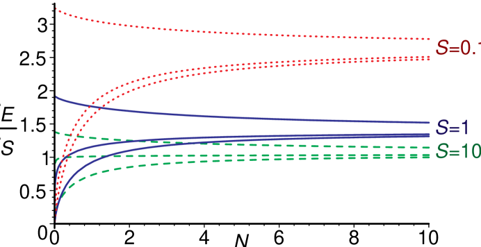
Figure 4: This figure shows the curves given by the ratio of capacities $C_{E}/C_{\rm{Shan}}$ for the quantum Gaussian channel with noise $N$ and the nine combinations of values: amplification/attenuation parameter $k=0.1$, $1$, or $3$; and signal strength $S=0.1$, $1$, or $10$. The dotted curves have $S=0.1$; the solid curves have $S=1$; and the dashed curves have $S=10$. Within each set, the curves have the values $k=0.1$, $k=1$, and $k=3$ from bottom to top.

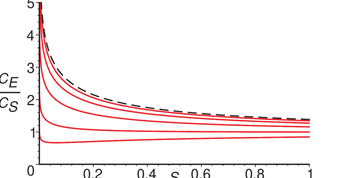
Figure 5: The solid curves show the ratio of capacities $C_{E}/C_{\mathrm{Shan}}$ for the quantum Gaussian channel with signal strength $S$, amplification/attenuation paramter $k=1$ and noise $N=0.1$, $0.3$, $1$, $3$, and $10$ (from bottom to top). The dashed curve is the limit of the solid curves as $N$ goes to $\infty$; namely, $C_{E}/C_{\mathrm{Shan}}=(S+1)\log(1+1/S)$. These curves approach $\infty$ as $S$ goes to $0$, and approach $1$ as $S$ goes to $\infty$.

The asymptotics of this formula are interesting. Let us hold the signal strength $S$ fixed, and let the noise $N$ go to infinity. Then,

$$\lim_{N\rightarrow\infty}\frac{C_{E}}{C_{\rm Shan}}=(S+1)\log\left(1+\frac{1}{S}\right),$$ (78)

which is independent of the attenuation/amplification parameter $k$. This ratio shows that the entanglement-assisted capacity can exceed the Shannon formula by an arbitrarily large factor, albeit when the signal strength $S$ is very small. We have plotted $C_{E}/C_{\rm{Shan}}$ for some parameters in Figs. 4 and 5.

Possibly a better comparison than that of $C_{E}$ to $C_{\mathrm{Shan}}$ would be that of $C_{E}$ to $C_{H}$, as $C_{H}$ is the best rate known for sending classical information over a quantum channel without use of shared entanglement, However, the optimal set of signal states to maximize $C_{H}$ for Gaussian channels is not known. For one-mode Gaussian channels with no squeezing, it is conjectured to be a thermal distribution of coherent states [18]; if this conjecture is correct, then $C_{H}\leq C_{\mathrm{Shan}}$ for these channels, so the ratio $C_{E}/C_{\mathrm{Shan}}$ underestimates $C_{E}/C_{H}$; see Fig. 6.

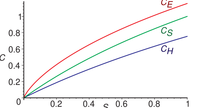
Figure 6: The values of the capacities $C_{E}$, $C_{\mathrm{Shan}}$, and the conjectured $C_{H}$ (in units of bits) are plotted for the Gaussian channel with signal strength $S$, noise $N=1$, and no amplification or attenuation ($k=1$). As the curves approach $0$, their leading-order behavior is as follows: $C_{H}\approx S$, $C_{\mathrm{Shan}}\approx(\log_{2}e)S$, and $C_{E}\approx-\frac{1}{2}S\log_{2}S$, so the ratios $C_{E}/C_{\mathrm{Shan}}$ and $C_{E}/C_{H}$ approach $\infty$ as $S$ goes to 0.

Some simple bounds on $C_{E}$ for the quantum Gaussian channel can be obtained using the techniques of [7]. Suppose that Alice takes a complex number $\alpha$, encodes it as the state ${|\alpha\rangle}$, and sends this through a quantum Gaussian channel. Bob then measures it in the coherent state basis. Here, the measurement step adds 1 to the noise, and this channel is thus equivalent to a classical Gaussian channel with average received signal strength $k^{2}S$, and average noise $N+1$ if $k\leq 1$, $N+k^{2}$ if $k\geq 1$. The quantum Gaussian channel must then have capacity greater than the capacity of this classical Gaussian channel. Conversely, Alice and Bob can simulate a quantum Gaussian channel by using a classical complex Gaussian channel: Alice measures her state (in the coherent state basis), sends the result through the classical channel, and Bob prepares a coherent state that depends on the signal he receives. If Alice starts with a state ${|\alpha\rangle}$, when she measures it, she obtains a complex number $\alpha+\epsilon$ where $\epsilon$ is a Gaussian with mean 0 and variance $1$. She can then multiply by $k^{2}$ to get $k^{2}\alpha+k^{2}\epsilon$. To simulate the quantum Gaussian channel, she must send this state through a classical channel with noise $N-k^{2}$ if $k\leq 1$, and $N-1$ if $k\geq 1$. This classical channel must then have classical capacity greater than $C_{E}$ for the quantum Gaussian channel it is simulating. The arguments in this paragraph thus give bounds of

$$\log\left(1+\frac{k^{2}S}{N+1}\right)\leq C_{E}\leq\log\left(1+\frac{S+1}{N/k^{2}-1}\right)$$ (79)

for $k\geq 1$, and of

$$\log\left(1+\frac{S}{N/k^{2}+1}\right)\leq C_{E}\leq\log\left(1+\frac{k^{2}(S+1)}{N-1}\right)$$ (80)

for $k\leq 1$. If we hold $S/N$ fixed, and let both these variables go to infinity, we find that these bounds all go to $\log(1+k^{2}S/N)$, which corresponds to the classical Shannon bound (since the signal strength at the receiver is $k^{2}S$).

If $k=1$, we can compute better bounds than these based on continuous-variable quantum teleportation and superdense coding. Alice and Bob can use a shared entangled squeezed state to teleport a continuous quantum variable [10], and can also use such a state for a superdense coding protocol involving one channel use per shared state that increases the classical capacity of a quantum channel [11]. The squeezed state used, with squeezing parameter $r\geq 0$, is expressed in the number basis as

$${|s_{r}\rangle}=\frac{1}{\cosh r}\sum_{j=0}^{\infty}(\tanh r)^{j}{|n_{A}=j\rangle}{|n_{B}=j\rangle},$$ (81)

where $n_{A}$ and $n_{B}$ are the photon numbers in Alice’s and Bob’s modes, respectively. This state is squeezed, which means that it cannot be represented as a mixture of coherent states with positive coefficients. In this state, the uncertainty in the difference of Alice and Bob’s position coordinates, $x_{A}-x_{B}$, is reduced, as is the uncertainty in the sum of their momentum coordinates $p_{A}+p_{B}$. The conjugate variables, $x_{A}+x_{B}$ and $p_{A}-p_{B}$, have increased uncertainty. If Alice and Bob measure their position coordinates, the difference of these coordinates is a Gaussian variable with mean $0$ and variance $e^{-2r}$, while the sum is a Gaussian with mean $0$ and variance $e^{2r}$. Similarly, if they measure their momentum coordinates, the sum has variance $e^{-2r}$ while the difference has variance $e^{2r}$. Further, if either Alice’s or Bob’s state is considered separately, it is a thermal state with average energy $\sinh^{2}r$.

In continuous-variable teleportation [10], Alice holds a state ${|t\rangle}$ she wishes to send to Bob, and one half of the shared state ${|s_{r}\rangle}$. She measures the difference of position coordinates of these states, $x_{m}=x_{t}-x_{A}$, and the sum of momentum coordinates, $p_{m}=p_{t}+p_{A}$. These are commuting observables, and so can be simultaneously determined. She sends these measurement outcomes to Bob, who then displaces his half of the shared state using $D(x_{m}+ip_{m})$.

Using continuous-variable teleportation, Alice can simulate a quantum Gaussian channel with $k=1$, average input energy $S$ and noise $N$ by sending the value $x_{m}+ip_{m}$ over a classical complex Gaussian channel with average input energy $S+(\cosh r)^{2}$ and noise $N-e^{-2r}$. This gives a bound equal to the classical capacity of this channel:

$$C_{E}\leq\log\left(1+\frac{S+(\cosh r)^{2}}{N-e^{-2r}}\right).$$ (82)

Finding the $r$ which minimizes this expression gives

$$e^{2r}=\frac{D_{1}+1}{N}$$ (83)

where

$$D_{1}=\sqrt{(N+1)^{2}+4NS}$$ (84)

is the value of the variable $D$ defined in Eq. (77) when we set $k=1$. This gives the bound

$$C_{E}\leq\log\left(1+\frac{S+(D_{1}+N+1)/(2N)}{N}\right).$$ (85)

Similarly, if Alice uses superdense coding [11] to send a continuous variable to Bob, her protocol simulates a classical Gaussian channel. The average energy input to this channel is $S-\sinh^{2}r$ and the noise is $N+e^{-2r}$, so we obtain the bound

$$C_{E}\geq\log\left(1+\frac{S-\sinh^{2}r}{N+e^{-2r}}\right).$$ (86)

Maximizing this expression, we find the maximum is at $e^{2r}=(D_{1}-1)/N$, and the bound obtained is

$$C_{E}\geq\log\left(1+\frac{S-(D_{1}-N-1)/(2N)}{N}\right).$$ (87)

Note that the bounds (82) and (86) reduce to the bounds of (79) and (80) when there is no entanglement in the squeezed state, i.e., when $r=0$.

B. The Amplitude Damping Channel

The amplitude damping channel describes a qubit channel which sends states which decay by attenuation from ${|1\rangle}$ to ${|0\rangle}$, but which do not undergo any other noise. This channel can be described by two Krauss operators,

$$A_{1}=\left(\begin{array}[]{cc}1&0\\ 0&\sqrt{1-p}\\ \end{array}\right)\rm{\ \ \ and\ \ \ }A_{2}=\left(\begin{array}[]{cc}0&\sqrt{p}\\ 0&0\\ \end{array}\right)$$

where

$${\cal N}:\rho\rightarrow\sum_{j=1}^{2}A_{j}\rho A_{j}^{\dagger}\,.$$

Figure 7: (a) The capacity functions $C_{E}$ and $C_{H}$ for the amplitude damping channel are plotted against the damping probability $p$. (b) The ratio $C_{E}/C_{H}$ is plotted. This curve is so steep near $p=1$ that for $p=1\!-\!10^{-50}$, the computed value of the ratio $C_{E}/C_{H}$ was only 3.8; the limiting value of 4 for $p=1$ was derived analytically.

The maximization over $\rho$ to find $C_{E}$ can be reduced to an optimization over one parameter, as symmetry considerations show that $\rho$ is of the form

$$\rho_{x}=\left(\begin{array}[]{cc}1-x&0\\ 0&x\end{array}\right),$$

This makes the optimization numerically tractable, and the dependence of $C_{E}$ on $p$ is shown in Fig. 7. As the damping probability $p$ goes to one, we can analytically find the highest-order term in the expression for $C_{E}$, giving

$$C_{E}\approx-x(1-p)\log(1-p)$$ (88)

for $0<x<1$. Here we use “$\approx$” to mean that the ratio of the two sides approaches 1 as $p$ goes to 1.

For the same channel, $C_{H}$ can also be obtained by optimizing over a one-parameter family which uses two signal states $\rho_{x,+}$ and $\rho_{x,-}$ with equal probability[16]. These signal states are

$$\rho_{x,\pm}=\left(\begin{array}[]{cc}1-x&\pm\sqrt{x(1-x)}\\ \pm\sqrt{x(1-x)}&x\end{array}\right).$$ (89)

As $p$ goes to one, again we can analytically find the highest-order term for $C_{H}$, which is

$$C_{H}\approx-x(1-x)(1-p)\log(1-p).$$ (90)

Thus, as $p$ goes to 1, the values of $x$ maximizing $C_{E}$ and $C_{H}$ respectively approach $1$ and $1/2$, and the ratio $C_{E}/C_{H}$ approaches four. These functions are shown graphically in Fig. 7. In our previous paper [7], we showed that for the qubit depolarizing channel, the ratio $C_{E}/C_{H}$ approached 3 as the depolarizing probability approached 1, and for the $d$-dimensional depolarizing channel, the ratio approached $d+1$. We do not know whether this ratio is bounded for finite-dimensional channels, although we suspect it to be. If so, then the interesting question arises of how this bound depends on the dimensions $\dim{\cal H}_{\rm{in}}$ and $\dim{\cal H}_{\rm{out}}$.

IV. Classical Reverse Shannon Theorem

Shannon’s celebrated noisy channel coding theorem established the ability of noisy channels to simulate noiseless ones, and allowed a noisy channel’s capacity to be defined as the asymptotic efficiency of this simulation. The reverse problem, of using a noiseless channel to simulate a noisy one, has received far less attention, perhaps because noisy channels are not thought to be a useful resource in themselves (for the same reason, there has been little interest in the reverse technology of water desalination—efficiently making salty water from fresh water and salt). We show, perhaps unsurprisingly, that any noisy discrete memoryless channel of capacity $C$ can be asymptotically simulated by $C$ bits of noiseless forward communication from sender to receiver, given a source $R$ of random information shared beforehand between sender and receiver. If this were not the case, characterization of the asymptotic properties of classical channels would require more than one parameter, because there would be cases where two channels of equal capacity could not simulate one another with unit asymptotic efficiency. In terms of the desalination analogy, water from two different oceans might produce equal yields of fresh drinking water, yet still not be equivalent because they produced unequal yields of partly saline water suitable, say, for car washing.

Although it is of some intrinsic interest as a result in classical information theory, we view the classical reverse Shannon theorem mainly as a heuristic aid in developing techniques that may eventually establish its quantum analog, namely the conjectured ability of all quantum channels of equal $C_{E}$ to simulate one another with unit asymptotic efficiency in the presense of shared entanglement.

Here we show that any classical discrete memoryless channel $N$, of capacity $C$, can be asymptotically simulated by $C$ uses of a noiseless binary channel, together with a supply of prior random information $R$ shared between sender and receiver.

The channel $N$ is defined by its stochastic transition matrix $N_{yx}$ between inputs $x\in\{1...d_{I}\}$ and outputs $y\in\{1...d_{O}\}$. Let $N^{n}$ denote the extended channel consisting of $n$ parallel applications of $T$, and mapping $x\in\{1...d_{I}^{n}\}$ to $y\in\{1...d_{O}^{n}\}$.

Theorem 2 (Classical Reverse Shannon Theorem)

Let $N$ be a DMC with Shannon capacity $C$ and $\epsilon$ a positive constant. Then for each block size $n$ there is a deterministic simulation protocol $S_{n}$ for $N^{n}$ which makes use of a noiseless forward classical channel and prior random information (without loss of generality a Bernoulli sequence $R$) shared between sender and receiver. When $R$ is chosen randomly, the number of bits of forward communication used by the protocol $S_{n}$ on channel input $x\in\{1...d_{I}\}^{n}$ is a random variable; let it be denoted $m_{n}(x)$. The simulation is exactly faithful in the sense that for all $n$ the stochastic matrix for $S_{n}$, when $R$ is chosen randomly, is identical to that for $N^{n}$,

$$\forall_{nxy}(S_{n})_{yx}=(N^{n})_{yx},$$ (91)

and it is asymptotically efficient in the sense that the probability that the protocol uses more than $n(C+\epsilon)$ bits of forward communication approaches zero in the limit of large $n$,

$$\lim_{n\rightarrow\infty}\max_{x\in\{1...d_{I}\}^{n}}P(m_{n}(x)>n(C+\epsilon))=0.$$ (92)

Note that the notion of simulation used here is stronger than the conventional one used in the forward version of Shannon’s noisy channel coding theorem, and in eq. (4) defining the generalized capacity of one quantum channel to simulate another. There the simulations are required only to be asymptotically faithful and their cost $m$ is deterministically upper bounded by $n(C+\epsilon)$. By contrast our simulations are exactly faithful for all $n$ and their cost is upper bounded by $n(C+\epsilon)$ only with probability approaching 1 in the limit of large $n$, for all $\epsilon>0$. To convert one of our simulations into a standard one, it suffices to discontinue the simulation and substitute an arbitrary output whenever $m_{n}(x)$ is about to exceed $n(C+\epsilon)$.

To illustrate the central idea of the simulation, we prove the theorem first for a binary symmetric channel (BSC), then extend the proof to a general discrete memoryless channel. Let $N$ be a binary symmetric channel of crossover probability $p$. Its capacity $C$ is $1\!-\!H_{2}(p)=1+p\log_{2}p+(1\!-\!p)\log_{2}(1\!-\!p)$. To prove the theorem in this case it suffices to show that for any rate $\epsilon>0$, there is a sequence of simulation protocols $S_{n}$ such that

$$\forall_{nxy}(S_{n})_{yx}=(N^{n})_{yx},$$ (93)

and

$$\lim_{n\rightarrow\infty}\max_{x\in\{1...d_{I}\}^{n}}P(m_{n}(x)>n(C+\epsilon))=0.$$ (94)

The simulation protocol $S_{n}$ is as follows:

1. Before receiving the input $x\in\{0,1\}^{n}$, Alice and Bob use the random information $R$ to choose a random set $Z(R,n)$ of $2^{n(C+\epsilon/2)}$ $n$-bit strings. [We use $\epsilon/2$, rather than $\epsilon$, to keep the total overhead, including other costs, below $\epsilon$].

2. Alice receives the $n$-bit input $x$.

3. Alice simulates the true channel $N^{n}$ within her laboratory, obtaining an $n$-bit “provisional output” $y$. Although this $y$ is distributed with the correct probability for the channel output, she tries to avoid transmitting $y$ to Bob, because doing so would require $n$ bits of forward communication, and she wishes to simulate the channel accurately while using less forward communication. Instead, where possible, she substitutes a member of the preagreed set $Z(R,n)$, as we shall now describe.

4. Alice computes the Hamming distance, $d=|x\!-\!y|$ between $x$ and $y$.

5. Alice determines whether there are any strings in the preagreed set $Z(R,n)$ having the same Hamming distance $d$ from $x$ as $y$ does. If so, she selects a random one of them, call it $y^{\prime}$, and sends Bob $0i$, where $i$ is the approximately $n(C+\epsilon/2)$-bit index of $y^{\prime}$ within the set $Z(R,n)$. If not, she sends Bob the string $1y$, the original unmodified $n$-bit string $y$, prefixed by a 1.

6. Bob emits $y^{\prime}$ or $y$, whichever he has received, as the final output of the simulation.

It can readily be seen that the probability of failure in step 5—i.e., of there being no string of the correct Hamming distance in the preagreed set $Z(R,n)$—decreases exponentially with $n$ as long as $\epsilon>0$. Thus the probability of needing to use more than $C(1+\epsilon)$ bits of forward communication approaches zero as required by Eq. (94). On the other hand, regardless of whether step 5 succeeds or fails, the final output is correctly distributed (satisfying Eq. (94)) since it has the correct distribution of Hamming distances from the input $x$, and, for each Hamming distance, is equidistributed among all strings at that Hamming distance from $x$. The theorem follows.

For a general discrete memoryless channel the protocol must be modified to take account of the nonbinary input and output alphabets, and the fact that the output entropy may be different for different inputs, unlike the BSC case. The notion of Hamming distance also needs to be generalized. The new protocol uses the notion of type class[13, 14]. Two $n$-character strings belong to the same type class if they have equal letter frequencies (for example four a’s, three b’s, twelve c’s etc.), and are therefore equivalent under some permutation of letter positions. We will consider input type classes (ITCs) and joint input/output type classes (JTC), the latter being defined as a set of input/output pairs (x,y) equivalent under some common permutation of the input and output letter positions. In other words, $(x_{1},y_{1})$ and $(x_{2},y_{2})$ belong to the same JTC if and only if there exists a permutation of letter positions, $\pi$, such that $\pi(x_{1})=x_{2}$ and $\pi(y_{1})=y_{2}$. Evidently, for any given input and output alphabet size, the number of ITCs, and the number of JTC are each polynomial in $n$. Let $k=1,2...K_{n}$ index the ITCs, and $\ell=1,2...L_{n}$ the JTC for inputs of length $n$. The JTC will be our generalization of the Hamming distance, since the transition probability $(N^{n})_{yx}$ is equal for all pairs $(x,y)$ in a given JTC. The new protocol follows:

1. Before receiving the input $x\in\{1,d_{I}^{n}\}$, Alice and Bob use the common random information $R$ to preagree on $K_{n}$ random sets $\{Z(R,n,k):k=1...K_{n}\}$ of $n$-letter output strings, one for each ITC. The set $Z(R,n,k)$ has cardinality $2^{n(C_{k}+\epsilon/2)}$, where $C_{k}<C$ is the channel’s capacity for inputs in the $k$’th ITC (in other words, $1/n$ times the channel’s input:output mutual information on $n$-letter inputs uniformly distributed over the $k$’th ITC). In contrast to the BSC case, where the members of $Z(R,n)$ were chosen randomly from a uniform distribution on the output space, the elements of $Z(R,n,k)$ are chosen randomly from the (in general nonuniform) output distribution induced by a uniform distribution of channel inputs over the $k$’th ITC.

2. Alice receives the $n$-letter input $x$, determines which ITC, $k$, it belongs to, and sends $k$ to Bob, using $o(n)$ bits to do so.

3. Alice simulates the true channel $N^{n}$ in her laboratory, obtaining an $n$-letter provisional output string $y$. Although this $y$ is distributed with the correct probability for the channel input $x$, she tries to avoid transmitting $y$ to Bob, because to do so would require too much forward communication. Instead she proceeds as described below.

4. Alice computes the index $\ell$ of the JTC to which the input/output pair $(x,y)$ belongs. As noted above, this JTC index is the generalization of the Hamming distance, which we used in the BSC case.

5. Alice determines whether there are any output strings in the preagreed set $Z(R,n,k)$ having the same JTC index relative to $x$ as $y$ does. If so, she selects a random one of them, call it $y^{\prime}$, and sends Bob the string $0i$ where $i$ is the approximately $n(C+\epsilon/2)$-bit index of $y^{\prime}$ within the set $Z(R,n,k)$. If not, she sends Bob the string $1y$.

6. Bob emits $y^{\prime}$ or $y$, whichever he has received, as the final output of the simulation.

This protocol deals with the problem of dependence of output entropy on input by encoding each ITC separately. Within any one ITC, the output entropy is independent of the input. The communication cost of telling Bob in which ITC the input lies is polylogarithmic in $n$, and so asymptotically negligible compared to $n$. Because one cannot increase the capacity of a channel by restricting its input, $nC$ is an upper bound the input:output mutual information $nC_{k}$ for inputs restricted to a particular ITC. Moreover, for any ITC $k$ and any input $x$ in that ITC, the input:output pairs generated by the true channel $T^{n}$, will be narrowly concentrated, for large $n$, on JTC whose transition frequencies approximate (to within $O(\sqrt{n}))$ their asymptotic values. Therefore, as before, for any $\epsilon>0$, the probability of failure in step 5 will decrease exponentially with $n$. And as before, the simulated transition probability $(S_{n})_{yx}$ on each ITC is exactly correct even for finite $n$. The reverse Shannon theorem for a general DMC follows, as does the following corollary.

Corollary 1 (Efficient simulation of one noisy channel by another)

In the presence of shared random information between sender and receiver, any two classical channels of equal capacity can simulate one another, in the sense of eq. (4), with unit asymptotic efficiency.

From the proof of the main theorem it can also be seen that when inputs to the noisy channel being simulated come from a source having a frequency distribution $q$ differing from the optimal one $p$ for which capacity $C$ is attained, then the asymptotic cost of simulating the channel on that source is correspondingly less.

Corollary 2 (Efficient simulation of noisy channels on constrained sources)

Let $N$ be a DMC, $q$ be a probability distribution over the source alphabet, and $I(N,q)$ be the channel’s constrained capacity, equal to the single-letter input:output mutual information on source $q$. Then, in the presence of shared random information $R$ between sender and receiver, the action of $N$ on any extended source having $q$ for each of its marginal distributions can be simulated in the manner of Theorem 2 with perfect fidelity and a forward noiseless communication cost asymptotically approaching $I(N,q)$: viz. $\forall_{\epsilon}\lim_{n\rightarrow\infty}P(m_{n}>n(I(N,q)+\epsilon))=0$. Here $m_{n}$ denotes the number of bits of forward communication used by the protocol when $R$ is chosen randomly with a uniform distribution and inputs are chosen randomly according to the constrained extended source.

V. Discussion—Quantum Reverse Shannon Conjecture

We conjecture (QRSC) that in the presence of unlimited shared entanglement between sender and receiver, all quantum channels of equal $C_{E}$ can simulate one another with unit asymptotic efficiency, in the sense of eq. (4). By the results of the previous section, the conjecture holds for classical channels (where the shared random information required for the classical reverse Shannon theorem is obtained from shared entanglement). In our previous paper [7] we showed that the QRSC also holds for another class of channels, the so-called Bell-diagonal channels, which commute with teleportation and superdense coding. For these channels, the single-use entanglement-assisted classical capacity of the channel via superdense coding is equal to the forward classical communication cost of simulating it via teleportation. The QRSC asserts this equality holds asymptotically for all quantum channels, even when (as for the amplitude damping channel) it is does not hold for single uses of the channel. We hope that the arguments used to prove the classical reverse Shannon theorem can be extended to demonstrate its quantum analog.

If the QRSC is true, one useful corollary would be the inability of a classical feedback channel from Bob to Alice to increase $C_{E}$. A causality argument shows that a feedback channel cannot increase $C_{E}$ for noiseless quantum channels. If we could simulate noisy quantum channels by noiseless ones, this would imply that if a feedback channel increased $C_{E}$ for any noisy channel, it would have to increase $C_{E}$ for noiseless ones as well, violating causality.

We thank Igor Devetak, David DiVincenzo, Alexander Holevo, Michael Nielsen and Barbara Terhal for helpful discussions, and the referees for careful reading and advice resulting in significant improvements.

References

- [1] N. Alon and J. H. Spencer, The Probabilistic Method, John Wiley and Sons, New York (1991).
- [2] A. Ashikhmin and E. Knill, “Nonbinary quantum stabilizer codes,” IEEE Trans. Inf. Theory 47, pp. 3065–3072 (2001); LANL eprint quant-ph/0005008.
- [3] H. Barnum, M. A. Nielsen, and B. Schumacher, “Information transmission through noisy quantum channels,” Phys. Rev. A 57, pp. 4153–4175 (1998); LANL eprint quant-ph/9702049.
- [4] H. Barnum, J. A. Smolin, and B. M. Terhal, “The quantum capacity is properly defined without encodings,” Phys. Rev. A 58, pp. 3496–3501 (1998); LANL e-print quant-ph/9711032.
- [5] C. H. Bennett, H. J. Bernstein, S. Popescu, and B. Schumacher, “Concentrating partial entanglement by local operations,” Phys. Rev. A 53, pp. 2046–2052 (1996).
- [6] C. H. Bennett, G. Brassard, C. Crépeau, R. Jozsa, A Peres and W. K. Wootters, “Teleporting an unknown quantum state via dual classical and EPR channels,” Phys. Rev. Lett. 70, pp. 1895–1899 (1993).
- [7] C. H. Bennett, P. W. Shor, J. A. Smolin, and A. V. Thapliyal, “Entanglement-assisted capacity of noisy quantum channels,” Phys. Rev. Lett. 83, pp. 3081–3084 (1999); LANL eprint quant-ph/9904023.
- [8] C. H. Bennett and P. W. Shor, “Quantum information theory,” IEEE Trans. Inform. Theory 44, pp. 2724–2742 (1998).
- [9] C. H. Bennett and S. J. Wiesner, “Communication via one- and two-particle operators on Einstein-Podolsky-Rosen states,” Phys. Rev. Lett. 69, pp. 2881–2884 (1992).
- [10] S. L. Braunstein and H. J. Kimble, “Teleportation of continuous quantum variables,” Phys. Rev. Lett. 80, pp. 869–872 (1998).
- [11] S. L. Braunstein and H. J. Kimble, “Dense coding with continuous quantum variables,” Phys. Rev. A 61, art. 042302 (2000).
- [12] N. Cerf and G. Adami, “Von Neumann capacity of noisy quantum channels, Phys. Rev. A 56, pp. 3470–3483 (1997).
- [13] Cover and Thomas, Elements of Information Theory, John Wiley and Sons, New York (1991).
- [14] I. Csiszár and J. Körner, Information Theory: Coding Theorems for Discrete Memoryless Systems, Akadémiai Kiadó, Budapest (1981).
- [15] D. P. DiVincenzo, T. Mor, P. W. Shor, J. A. Smolin and B. M. Terhal, “Unextendible product bases, uncompletable product bases, and bound entanglement,” Phys. Rev. Lett. 82, pp. 5385-5388, (1999); LANL eprint quant-ph 9908070.
- [16] C. A. Fuchs, personal communication.
- [17] P. Hausladen, R. Jozsa, B. Schumacher, M. Westmoreland, and W. K. Wootters, “Classical information capacity of a quantum channel,” Phys. Rev. A 54, pp. 1869–1876 (1996).
- [18] A. S. Holevo and R. F. Werner “Evaluating capacities of bosonic Gaussian channels,” Phys. Rev. A 63, art. 032313 (2001); LANL eprint quant-ph/9912067.
- [19] A. S. Holevo, “The capacity of the quantum channel with general signal states,” IEEE Trans. Information Theory 44, pp. 269–273 (1998).
- [20] A. S. Holevo, “On entanglement-assisted classical capacity,” LANL eprint quant-ph/0106075.
- [21] P. Horodecki, M. Horodecki, and R. Horodecki, “Binding entanglement channels,” J. Modern Optics 47, pp. 347–354 (2000), LANL eprint quant-ph/9904092.
- [22] L. P. Hughston, R. Jozsa, W. K. Wootters, “A complete classification of quantum ensembles having a given density matrix,” Phys. Lett. A 183, pp. 14-18 (1993).
- [23] R. Jozsa and B. Schumacher, “A new proof of the quantum noiseless coding theorem,” J. Modern Optics 41, pp. 2343–2350 (1994).
- [24] C. King, “Additivity for unital qubit channels,” J. Math. Phys., to appear; LANL eprint quant-ph/0103156.
- [25] E. Lieb and M.B. Ruskai, “Proof of the Strong Subadditivity of Quantum Mechanical Entropy” J. Math. Phys. 14, pp. 1938–1941 (1973).
- [26] G. Lindblad, “Quantum entropy and quantum measurements,” in Quantum aspects of optical communications, Lecture Notes in Physics 378, C. Bendjaballah, O. Hirota, S. Reynaud (eds.) Springer, pp. 71–80 (1991).
- [27] H.-K. Lo and S. Popescu, “The classical communication cost of entanglement manipulation: Is entanglement an inter-convertible resource?” Phys. Rev. Lett. 83, pp. 1459–1462 (1999); LANL eprint quant-ph/9902045.
- [28] M. A. Nielsen and I. L. Chuang, Quantum Computation and Quantum Information, Cambridge University Press, Cambridge, UK, 2000.
- [29] B. Schumacher, “Quantum coding,” Phys. Rev. A 51, pp. 2738–2747 (1995).
- [30] B. W. Schumacher and M. A. Nielsen, “Quantum data processing and error correction”, Phys. Rev. A 54, pp. 2629–2635, (1996).
- [31] B. Schumacher and M. D. Westmoreland, ”Sending classical information via noisy quantum channels,” Phys. Rev. A 56, pp. 131–138 (1997).
- [32] G. Vidal and J. I. Cirac, “Irreversibility in asymptotic manipulations of entanglement,” Phys. Rev. Lett. 86, pp. 5803-5806 (2001); LANL eprint quant-ph/0102036.
- [33] D. F. Walls and G. J. Milburn, Quantum Optics, Springer Verlag, Berlin (1994).
- [34] A. Wehrl, “General properties of entropy,” Rev. Mod. Phys. 40 pp. 221–260 (1978).