Schrödinger-picture correlation functions for nonlinear evolutions

Abstract

The well known interpretational difficulties with nonlinear Schrödinger and von Neumann equations can be reduced to the problem of computing multiple-time correlation functions in the absence of Heisenberg picture. Having no Heisenberg picture one often resorts to Zeno-type reasoning which explicitly involves the projection postulate as a means of computing conditional and joint probabilities. Although the method works well in linear quantum mechanics, it completely fails for nonlinear evolutions. We propose an alternative way of performing the same task in linear quantum mechanics and show that the method smoothly extends to the nonlinear domain. The trick is to use appropriate time-dependent Hamiltonians which involve “switching-off functions”. We apply the technique to the EPR problem in nonlinear quantum mechanics and show that paradoxes of Gisin and Polchinski disappear.

I Introduction

Ten years ago Polchinski published a paper [1] where he showed how to avoid unphysical influences between separated systems in nonlinear quantum mechanics. The paper was a response to criticisms of Kibble-Weinberg nonlinear quantum mechanics [2, 3] raised by Gisin [4] and one of us [5]. Polchinski proposed to eliminate the problem by eliminating its source, the projection postulate, and resorting to the Many Worlds Interpretation. However, after having eliminated one difficulty he showed that there appears another one, a kind of weird communication between different Everett worlds.

The paper had several implications. First of all, it convinced a large group of physicists working on foundations of quantum mechanics, including Weinberg himself (see his remarks in [6]), that linearity is an ultimate element of all the possible “final theories”.

On the other hand, the Polchinski multiparticle extension showed that at least part of difficultes trivally disappears if one starts with nonlinear evolutions formulated in terms of von Neumann-type equations. Looking at the von Neumann dynamics as a classical Hamiltonian system on a Poisson manifold of states represented by reduced density matrices, one arrives at a surprisingly elegant formalism [7, 8, 9, 10, 11, 12] which goes much beyond the original Weinberg proposal. Theories so constructed led to new families of integrable von Neumann equations which turned out to be very interesting in themselves at least from the point of view of integrable systems [13, 14, 15, 16, 17].

In spite of the original problems with the Weinberg formalism notable developments were reported by groups working on “geometric quantum mechanics” [18, 19, 20]. Quantum mechanics, when looked at from a geometric standpoint, turns out to be a classical theory “living” on a very symmetric phase space (a Kähler manifold with maximal symmetries). It becomes quite natural, then, to think of standard quantum mechanics as an analogue of a “vacuum” spacetime from general relativity. Since the most interesting spacetimes are those which are less symmetric, maybe the same will be true for quantum mechanics? An unquestionable beauty of the geometric perspective suggests that these possibilities should be further investigated.

Yet another road to nonlinear Schrödinger equations was discovered by Goldin and Doebner [21, 22, 23, 24]. Studying representations of groups of diffeomorphisms they noticed that there exists a class of representations parametrized by the real number $D$ which has an interpretation of a diffusion coefficient [25, 26]. All the other representations had a clear physical interpretation. They were known to unify the description of an extraordinary variety of quantum systems and generated some physical predictions difficult to reach by other means (e.g. the anyon statistics in two-dimensional space). However, this particular class resisted a quantum mechanical interpretation until it was realized that it corresponds to a family of nonlinear dissipative Schrödinger equations earlier derived in the context of quantum chemistry by Schuch and his collaborators [27]. Doebner and Goldin subsequently introduced the group of nonlinear gauge transformations necessary to understand the resulting theory. The resulting formalism was shown to contain as special cases nonlinear modifications of quantum mechanics proposed independently by other researchers [28, 29, 30, 31, 32, 33, 34] It became clear that linearity is a gauge-dependent property and a simple rule “linear good, nonlinear bad” is oversimplified.

Quite recently it turned out that dynamics of certain $D$-branes leads to nonlinear Schrödinger equations od the Doebner-Goldin type [35, 36] and the von Neumann-type nonlinearities introduced in [11] have links with nonextensive statistics [37, 38, 39].

In spite of the optimism of the groups we have mentioned not everyone was fully satisfied by the Many Worlds solution. Gisin openly disqualified nonlinear Schrödinger equations as “irrelevant” [40]. Goldin [41] did not agree with Gisin but formulated a series of doubts with respect to the Polchinski solution pointing out, in particular, that multiparticle extensions of physically equivalent theories but performed in different nonlinear gauges lead to physically inequivalent results. Also Mielnik in a recent paper [42] argued on general grounds that the difficulties remain.

As a result, a person who wants to understand the current state of knowledge about nonlinear generalizations of quantum mechanics will find a complete spectrum of mutually contradicting statements.

We think that three main questions are causing the entire embarassment. One is the unclear role of nonlinear averages and eigenvalues if nonlinear observables are involved. The other is the role of density matrices (“mixed” states) in nonlinear formalism. Finally, an open question is how to compute joint probabilities in EPR-type experiments.

The main topic of the present paper is the third issue. Two applications of nonlinear averages are discussed in the Appendix. We do not address the problem of density matrices. We believe that a common error one finds in the literature on nonlinear Schrödinger equations is to treat solutions of von Neumann-type equations as states which are mixed in the standard sense of mixed states on a phase space [43]. To the best of our knowledge no approach based on Schrödinger-type equations was able to successfully address the question of composite systems. This should be contrasted with the formalism based on von Neumann equations which, up to a few interpretational subtleties which are a subject of the present work, simply does not lead to this difficulty.

In what follows we formulate a new operational framework for interpretation of experiments in both linear and nonlinear quantum systems. We do not use the Many Worlds Interpretation and hence do not have the “Everett phone”. On the other hand we make a very restrictive use of the projection postulate. We allow to use projections only in two cases: (1) to determine initial conditions and (2) at the moments particles are detected and destroyed (final conditions).

The question that arises, then, is how to describe situations where there are, say, two correlated particles and one of them is destroyed by a detector at time $t=t_{1}$ whereas the other one is allowed to evolve until it gets destroyed at $t=t_{2}>t_{1}$. This is what we call a two-time measurement. A typical solution, known also as a quantum Zeno effect, is to regard the second particle as evolving for $t_{1}<t<t_{2}$ with a new initial condition produced by an appropriate projection-at-a-distance at $t=t_{1}$.

We exclude this approach since in application to nonlinear evolutions of entangled states it leads to serious complications. Instead, we reformulate the standard strategy with the help of “switching-off functions” and show that (1) in the linear case the result is identical to the standard Zeno-type calculation and (2) in nonlinear case is free from unphysical influences between correlated particles and, hence, ultimately eliminates the “EPR phone”.

We will begin with a few remarks on filters and histories. The notion of a filter often occurs in the context of conditional probabilities and the projection postulate. However, there exists also a desription where filters are described in terms of unitary matrices and do not lead to irreversible projections. This point is essential for our argument. In the next two sections we discuss the role of the projection postulate for two-time measurements and point out the role of “switching-off functions”. In Sec. V we discuss problems with two-time measurements in presence of nonlinearities. Sec. VI discusses Polchinski’s multi-particle extension and its modification in terms of switching-off functions. In Sec. VII we explicitly solve an example and compare the standard projection-based calculation with the new proposal. Sec. VIII discusses implications of our approach for the question of teleportation. Arguments are given that one should not identify pre- and post-selected ensembles if nonlinear evolutions are involved. The point is essential since a true teleportation corresponds to a pre-selected ensemble whereas ordinary correlation experiments involve post-selections.

We end with the Appendix on nonlinear averages, the use of them in information theory and nonextensive statistics, and their links with the subject of the paper.

II Histories and filters

A typical quantum history is shown in Fig. 1. A particle produced by a source undergoes a series of scattering events, represented by unitary evolutions $U_{1}$ and $U_{2}$. Before, between and after the scattering the evolution is free, say. The particle may, for simplicity, be regarded as a two level system and the $U$s as some sorts of beam splitters (mirrors, analyzers of polarizaton, Stern-Gerlach magnets,…). There are several outgoing channels, and each of the channels corresponds to a different result of the experiment.

The probability of detection in, say, channel 1 can be calculated in a couple of different ways. One way of doing this is to compute the overall evolution operator $V(t)$, including the whole evolution from the source till detection, and calculate the probability

$$p_{1} = {\,\rm Tr\,}\big{(}E_{2}V(t)\rho(0)V(t)^{{\dagger}}\big{)}$$ (1)

$$= {\,\rm Tr\,}\big{(}E_{2}\rho(t)\big{)}$$ (2)

where $E_{2}$ is an appropriate projector operator.

Another way is to split the evolution into pieces explicitly involving the scattering matrices $U_{k}$ and a free evolution between them. The $U$s play here a role of analyzers of the properties represented by projection operators $E_{k}$ and ${{}^{\perp}E}_{k}$, $E_{k}+{{}^{\perp}E}_{k}=I$. Denote by $U(t-t^{\prime})$ the free evolution between times $t$ and $t^{\prime}$. Since it satisfies the group composition property

$$U(t-t^{\prime})=U(t^{\prime})^{{\dagger}}U(t).$$ (3)

we find

$$p_{1} = {\,\rm Tr\,}\Big{(}U(t-t_{2})E_{2}U(t_{2}-t_{1})E_{1}U(t_{1})\rho(0)U(t_{1})^{{\dagger}}E_{1}U(t_{2}-t_{1})^{{\dagger}}E_{2}U(t-t_{2})^{{\dagger}}\Big{)}$$ (4)

$$= {\,\rm Tr\,}\Big{(}E_{2}(t_{2})E_{1}(t_{1})\rho(0)E_{1}(t_{1})E_{2}(t_{2})\Big{)}$$ (5)

where $E_{k}(t_{k})=U(t_{k})^{{\dagger}}E_{k}U(t_{k})$. Expression (5) is often called a history [48]. In quantum-optics literature one would rather speak of a two-time correlation function. In derivation of (4) one makes an explicit use of the unitarity of evolution whereas the transition from (4) to (5) involves (3). On the other hand, the form (2) is more general and can survive even if the dynamics $t\mapsto\rho(t)$ is nonlinear.

It is an appropriate moment to point out that one should not treat the first splitting of the beam by $U_{1}$ as a measurement of the property $E_{1}$. The measurement occurs when the particle vanishes in the detector and produces a click. Before that moment the evolution is unitary and reversible. After the measurement the measured particle is destroyed and is no longer under the jurisdiction of quantum mechanics.

Our beam splitters $U_{k}$ are examples of devices which are sometimes referred to as filters [49]. As we have seen, the derivation of the history (5) explicitly employed the fact that, for calculational purposes, filters can be represented by projectors and, hence, by non-unitary operators. However, it is extremely important to understand that the same physical process can be described by the exact formula (2) which describes propagation of particles through filters in a unitary way.

In such a formulation projectors are applied only twice — at the very beginning when one selects a concrete initial condition, and at the very end where the particle is detected and destroyed.

III Entangled states and two-time measurements

Two-time measurements are at the heart of difficulties with nonlinear extensions of quantum mechanics. We begin with their orthodox description in linear quantum mechanics.

Consider a two-electron system initially prepared in the singlet state

$$|\Psi(0)\rangle = \frac{1}{\sqrt{2}}\Big{(}|+\rangle|-\rangle-|-\rangle|+\rangle\Big{)}$$ (6)

and whose Hamiltonian is

$$H = H_{1}\otimes I_{2}+I_{1}\otimes H_{2}.$$ (7)

The dynamics of the state is

$$|\Psi(t)\rangle = V_{1}(t)\otimes V_{2}(t)|\Psi(0)\rangle.$$ (8)

where $V_{k}(t)=\exp(-iH_{k}t)$. It is known that $|\Psi(0)\rangle$ will be unchanged if $V_{1}=V_{2}$. However, if $H_{1}\neq H_{2}$ the perfect initial anti-correlation of spins holding at $t=0$ will be lost at later times.

Now let us imagine that two measurements of the $z$-components of spin are performed; one at time $t=t_{1}$ on particle $\#1$, and the other at $t=t_{2}>t_{1}$ on particle $\#2$. We want to calculate an average of the observable $\sigma_{z}\otimes\sigma_{z}$.

Denoting by $E_{\pm}\otimes I$ and $I\otimes E_{\pm}$ the appropriate projectors we can proceed as follows.

• At $t=t_{1}$ project

  $$|\Psi(t_{1})\rangle\mapsto\frac{E_{\pm}\otimes I|\Psi(t_{1})\rangle}{\parallel E_{\pm}\otimes I|\Psi(t_{1})\rangle\parallel}$$ (9)

• Evolve the resulting state by

  $$\frac{E_{\pm}\otimes V_{2}(t_{2}-t_{1})|\Psi(t_{1})\rangle}{\parallel E_{\pm}\otimes I|\Psi(t_{1})\rangle\parallel}$$ (10)

• Calculate at $t=t_{2}$ the (conditional) probabilities

  $$\frac{\langle\Psi(t_{1})|E_{\pm}\otimes V_{2}(t_{2}-t_{1})^{{\dagger}}E_{\pm^{\prime}}V_{2}(t_{2}-t_{1})|\Psi(t_{1})\rangle}{\langle\Psi(t_{1})|E_{\pm}\otimes I|\Psi(t_{1})\rangle}$$ (11)

• The denominator in (11) is the probability of finding $\pm 1$ for the first particle at $t=t_{1}$. Therefore the joint probability of finding $\pm$ for the first particle and $\pm^{\prime}$ for the second one is the numerator of (11), i.e.

  $$\langle\Psi(0)|V_{1}(t_{1})^{{\dagger}}E_{\pm}V_{1}(t_{1})\otimes V_{2}(t_{2})^{{\dagger}}E_{\pm^{\prime}}V_{2}(t_{2})|\Psi(0)\rangle.$$ (12)

The second step (10) was done in this way since we knew already the result of one measurement after (9). The result created an initial condition for the remaining dynamics of the other particle at $t=t_{1}$ (this is essentially the quantum Zeno effect). The projection postulate has therefore explicitly been used in the second step at $t=t_{1}$.

The formula (12) is again a correlation function. Let us note that we would get the same formula if we computed the average of the projector

$$E_{\pm}\otimes E_{\pm^{\prime}}$$ (13)

in the state

$$V_{1}(t_{1})\otimes V_{2}(t_{2})|\Psi(0)\rangle.$$ (14)

An identical result would have been obtained if one considered the time dependent Hamiltonian

$$H_{t_{1},t_{2}}(t) = \theta(t-t_{1})H_{1}\otimes I_{2}+\theta(t-t_{2})I_{1}\otimes H_{2}.$$ (15)

were the $\theta(x)$s is the step function equal 1 for $x<0$ and 0 otherwise, and computed the average of (13) in the state

$$|\Psi_{t_{1},t_{2}}(t)\rangle=e^{-iH_{1}\otimes I_{2}\int_{0}^{t}\theta(\tau-t_{1})d\tau-iI_{1}\otimes H_{2}\int_{0}^{t}\theta(\tau-t_{2})d\tau}|\Psi(0)\rangle.$$ (16)

The times $t_{1}$ and $t_{2}$ play a role of parameters describing the system. They naturally incorporate into the formalism the presence of detectors and the fact that detections are registered at certain times.

It is easy to understand why the energy of the particles is not conserved during the dynamics: At the moments the particles “get frozen” by the detection process their energies are transferred to the detectors. Only the composite system “particles plus detectors” is closed.

It is also obvious that one should not apply “switching-off functions” $\theta$ for acts of filtering that do not end up in a detection and destruction, such as those denoted by $U_{1}$ and $E_{1}$ at Fig. 1.

IV Two-time measurements on beams of pairs

In real experiments one deals with beams of pairs. A beam consisting of $N$ pairs is a tensor product of $N$ copies of single-pair states. Real experiments do not produce all the pairs at the same initial $t=0$. An experiment may run for weeks, therefore it is much more realistic to impose initial conditions on each of the pairs separetely and at different times: $t_{0}^{1},\dots,t_{0}^{N}$.

A run consisting of $N$ pairs of detections at times $(t_{1}^{1},t_{2}^{1})$, … $(t_{1}^{N},t_{2}^{N})$, can be described by the state vector

$$|\Psi_{\{t_{0}^{i},t_{1}^{i},t_{2}^{i}\}}(t)\rangle = |\Psi_{t_{0}^{1},t_{1}^{1},t_{2}^{1}}(t)\rangle\otimes\dots\otimes|\Psi_{t_{0}^{N},t_{1}^{N},t_{2}^{N}}(t)\rangle.$$ (17)

If experimental conditions do not change during the run one may parametrize (17) by times of flight $\Delta t_{k}^{i}=t_{k}^{i}-t_{0}^{i}$.

Observables, such as the one from the previous section are now represented in a frequency form i.e.

$$F_{N}(\sigma_{z}\otimes\sigma_{z}) = \frac{1}{N}\Big{(}(\sigma_{z}\otimes\sigma_{z})\otimes(I\otimes I)\otimes\dots\otimes(I\otimes I)+\dots+(I\otimes I)\otimes\dots\otimes(I\otimes I)\otimes(\sigma_{z}\otimes\sigma_{z})\Big{)}.$$ (18)

One can show [50, 51] that frequency operators of the form (18) naturally imply quantum mechanical laws of large numbers (both weak and strong).

Let us note that the sub-beam of $N$ particles $\#1$ (i.e. those going to the “left”) is described by the product of reduced density matrices

$$\rho_{\{t_{0}^{i},t_{1}^{i}\}}(t) = \rho_{t_{0}^{1},t_{1}^{1}}(t)\otimes\dots\otimes\rho_{t_{0}^{N},t_{1}^{N}}(t)$$ (19)

which does not depend on times of detection of particles $\#2$. This follows trivially from the fact that reduced density matrices of particles $\#1$ do not depend on the form of Hamiltonian of particles $\#2$, the fact whether the Hamiltonians are time-dependent or not being irrelevant. The switching-off functions are an element of definition of the Hamiltonians.

Following exactly the same reasoning we can describe ensembles of $n$-tuples of particles and the associated $n$-time measurements.

V Two-time measurements for entangled states in nonlinear quantum mechanics

The above discussion does not really bring anything technically new if one sticks to linear evolutions of states.

However, if nonlinear evolutions are involved the first two steps of our analysis, (9) and (10), are doubtful. The reason is that it is not clear whether the masurement performed on particle $\#1$ should be just a simple projection producing a new initial condition at $t=t_{1}$ for particle $\#2$. In linear quantum mechanics the projected state is an eigenvector. In nonlinear theory there are many inequivalent definitions of eigenvectors [9]. Moreover, if Doebner-Goldin equations are concerned the projection postulate should be formulated in a gauge independent way [45]

Another point is that nonlinear dynamics is very sensitive to modifications of initial conditions and in the generic case the reduced density matrix of particle $\#2$ will depend on the choice of both $t_{1}$ and the projector which performs the reduction. The well known Gedankenexperiment of Gisin [4] is precisely a two-time measurement involving steps (9)-(10) and a nonlinear evolution for $t_{1}<t<t_{2}$. It is known to predict an unphysical behavior of the particles and some kind of “faster-than-light” effect.

One should know that an appropriately (or, rather, inappropriately) defined nonlinear dynamics of entangled states can produce similar unphysical phenomena [5] even if one does not explicitly use the projection postulate at the level of solutions. The Weinberg formalism [3] incorporates the projection postulate already at the level of Hamiltonian function of the composite system. In this way one defines a multiparticle nonlinear Schrödinger equation whose solutions imply probabilities one would have derived from the two step procedure (9)-(10).

It was shown later by Polchinski [1] and others [8, 10] how to redefine the dynamics in a way which eliminates the unwanted properties of the Weinberg formalism. To get rid of the unphysical effect associated with the projection postulate Polchinski decided to eliminate the projection postulate itself. But then it turned out that strange effects occur at the level of the Many Worlds Interpretation and the “EPR phone” is replaced by an “Everett phone”. One cannot completely disagree with those who are not yet fully satisfied by the Polchinski formulation [6, 4, 41, 42]

In the next section we propose a new framework, a sort of “golden middle” between Gisin and Polchinski. Although we keep the projection postulate and do not need Many Worlds (hence no Everett phone) we nevertheless maintain the local propeties of the Polchinski formalism (no EPR phone).

VI Switching-off-function modification of Polchinski’s multiparticle extension

Nonlinear dynamics in the Weinberg-Polchinski quantum mechanics is given by Schrödinger equations associated with non-bilinear Hamiltonian functions,

$$i\dot{\psi}_{k} = \frac{\partial{\cal H}(\psi,\bar{\psi})}{\partial\bar{\psi}_{k}}.$$ (20)

It is essential that not all the possible Hamiltonian functions are acceptable. One accepts only those ${\cal H}(\psi,\bar{\psi})$ which can be written as

$${\cal H}(\psi,\bar{\psi})={\cal H}(\rho)\big{|}_{\rho=|\psi\rangle\langle\psi|}.$$ (21)

For example

$${\cal H}(\psi,\bar{\psi}) = {\cal H}(\psi_{+},\psi_{-},\bar{\psi}_{+},\bar{\psi}_{-})$$ (22)

$$= (\psi_{+}\bar{\psi}_{-}+\psi_{-}\bar{\psi}_{+})^{2}=\langle\psi|\sigma_{x}|\psi\rangle^{2}=({\,\rm Tr\,}\rho\sigma_{x})^{2}\big{|}_{\rho=|\psi\rangle\langle\psi|}$$ (23)

is acceptable, whereas

$${\cal H}(\psi,\bar{\psi}) = (\psi_{+}\psi_{-}+\bar{\psi}_{-}\bar{\psi}_{+})^{2}$$ (24)

is not (as opposed to the acceptable functions the latter is not invariant under $|\psi\rangle\mapsto e^{i\alpha}|\psi\rangle$). In linear quantum mechanics all Hamiltonian functions can be written as

$${\cal H}(\psi,\bar{\psi}) = \langle\psi|H|\psi\rangle={\,\rm Tr\,}\rho H\big{|}_{\rho=|\psi\rangle\langle\psi|}$$ (25)

and, hence, are acceptable.

If we have two such particles each described by its own Hamiltonian function

$${\cal H}_{1}(\psi_{1},\bar{\psi}_{1}) = {\cal H}_{1}(\rho)\big{|}_{\rho=|\psi_{1}\rangle\langle\psi_{1}|},$$ (26)

$${\cal H}_{2}(\psi_{2},\bar{\psi}_{2}) = {\cal H}_{2}(\rho)\big{|}_{\rho=|\psi_{2}\rangle\langle\psi_{2}|},$$ (27)

then the two-particle Hamiltonian function is simply their sum evaluated in appropriate one-particle states of particles $\#1$ and $\#2$, respectively.

What makes this formulation ingeniously simple is the fact that for a generic entangled state

$$|\Psi\rangle = \sum_{k_{1}k_{2}}\Psi_{k_{1}k_{2}}|k_{1}\rangle|k_{2}\rangle$$ (28)

representing the two-particle system, states of the one particle subsystems may be represented by reduced density matrices

$$\rho_{1} = \sum_{k_{1}l_{1}k_{2}}\bar{\Psi}_{k_{1}k_{2}}\Psi_{l_{1}k_{2}}|k_{1}\rangle\langle l_{1}|,$$ (29)

$$\rho_{2} = \sum_{k_{1}k_{2}l_{2}}\bar{\Psi}_{k_{1}k_{2}}\Psi_{k_{1}l_{2}}|k_{2}\rangle\langle l_{2}|.$$ (30)

Due to the above mentioned acceptability condition it makes sense to consider

$${\cal H}_{1+2}(\Psi,\bar{\Psi}) = {\cal H}_{1}(\rho)\big{|}_{\rho_{1}}+{\cal H}_{2}(\rho)\big{|}_{\rho_{2}}.$$ (31)

The two-particle Schrödinger equation has again the Hamilton form

$$i\dot{\Psi}_{k_{1}k_{2}} = \frac{\partial{\cal H}_{1+2}(\Psi,\bar{\Psi})}{\partial\bar{\Psi}_{k_{1}k_{2}}}.$$ (32)

Having found its solution we can write with its help reduced density matrices of the subsystems. It can be shown in several different ways and at different levels of generality [1, 8, 11, 10] that the dynamics of a reduced density matrix of one of those subsystems is independent of the choice of Hamiltonian function of the other subsystem. Therefore it is not posible to influence particle $\#1$ by measurements performed on particle $\#2$, and vice versa. This establishes locality of the formalism.

Applying the above technique to the EPR situation we have no difficulty with describing measurements of, say, $\sigma_{z}\otimes\sigma_{z}$ if the measurements are performed at the same time $t=t_{1}=t_{2}$. The formula for probabilities is the standard one:

$$\langle\Psi(t)|E_{\pm}\otimes E_{\pm^{\prime}}|\Psi(t)\rangle.$$ (33)

But what about two-time measurements? We do not have to our disposal the projection at $t_{1}$ since we know that it will produce unphysical nonlocal effects.

What we can do, however, is to resort to the switching-off function formulation which, as we have shown above, is equivalent to the one based on the projection postulate in the linear case. We define the two particle Hamiltonian function by

$${\cal H}_{t_{1},t_{2}}(t,\Psi,\bar{\Psi}) = \theta(t-t_{1}){\cal H}_{1}(\rho)\big{|}_{\rho_{1}}+\theta(t-t_{2}){\cal H}_{2}(\rho)\big{|}_{\rho_{2}}.$$ (34)

The Schrödinger equation for two particles is again

$$i\dot{\Psi}_{k_{1}k_{2}} = \frac{\partial{\cal H}_{t_{1}t_{2}}(t,\Psi,\bar{\Psi})}{\partial\bar{\Psi}_{k_{1}k_{2}}}.$$ (35)

It is important that, similarly to the linear case, the reduced density matrices of the subsystems depend only on their “own” $t_{i}$s. This is a straightforward consequence of locality of the Polchinski formulation.

VII Example: Evolution of a pair of spin-1/2 particles

The Hamiltonian functions in this example are

$${\cal H}_{1}(\psi_{1},\bar{\psi}_{1}) = A\langle\psi_{1}|\sigma_{z}|\psi_{1}\rangle^{2}/2$$ (36)

$${\cal H}_{2}(\psi_{2},\bar{\psi}_{2}) = B\langle\psi_{2}|\sigma_{z}|\psi_{2}\rangle^{2}/2.$$ (37)

The Polchinski two-particle extension is

$${\cal H}_{1+2}(\Psi,\bar{\Psi}) = A\langle\Psi|\sigma_{z}\otimes I|\Psi\rangle^{2}/2+B\langle\Psi|I\otimes\sigma_{z}|\Psi\rangle^{2}/2$$ (38)

and the two-particle Schrödinger equation derived from this Hamiltonian function is

$$i|\dot{\Psi}\rangle = \Big{(}A\langle\Psi|\sigma_{z}\otimes I|\Psi\rangle\sigma_{z}\otimes I+B\langle\Psi|I\otimes\sigma_{z}|\Psi\rangle I\otimes\sigma_{z}\Big{)}|\Psi\rangle.$$ (39)

Our modification is

$${\cal H}_{t_{1},t_{2}}(\Psi,\bar{\Psi}) = \theta(t-t_{1})A\langle\Psi|\sigma_{z}\otimes I|\Psi\rangle^{2}/2+\theta(t-t_{2})B\langle\Psi|I\otimes\sigma_{z}|\Psi\rangle^{2}/2$$ (40)

and

$$i|\dot{\Psi}\rangle = \Big{(}\theta(t-t_{1})A\langle\Psi|\sigma_{z}\otimes I|\Psi\rangle\sigma_{z}\otimes I+\theta(t-t_{2})B\langle\Psi|I\otimes\sigma_{z}|\Psi\rangle I\otimes\sigma_{z}\Big{)}|\Psi\rangle,$$ (41)

with the general solution

$$|\Psi_{t_{1},t_{2}}(t)\rangle = e^{-iA\langle\Psi(0)|\sigma_{z}\otimes I|\Psi(0)\rangle\sigma_{z}\otimes I\int_{0}^{t}\theta(\tau-t_{1})d\tau-iB\langle\Psi(0)|I\otimes\sigma_{z}|\Psi(0)\rangle I\otimes\sigma_{z}\int_{0}^{t}\theta(\tau-t_{2})d\tau}|\Psi(0)\rangle$$ (42)

$$= e^{-iA\langle\sigma_{z}(0)\rangle_{1}\sigma_{z}\kappa(t,t_{1})}\otimes e^{-iB\langle\sigma_{z}(0)\rangle_{2}\sigma_{z}\kappa(t,t_{2})}|\Psi(0)\rangle$$ (43)

where $\langle\sigma_{z}(0)\rangle_{k}={\,\rm Tr\,}(\rho_{k}(0)\sigma_{z})$, $\kappa(t,t_{k})=\int_{0}^{t}\theta(\tau-t_{k})d\tau$. (43) describes the entire history of the two particles: From their “birth” at $t=0$ to their “deaths” at $t=t_{1}$ and $t=t_{2}$. The standard Polchinski solution is recovered in the limits $t_{1},t_{2}\to+\infty$.

There is absolutely no ambiguity in the switching-off-function formulation. An experimentalist who wants to know what are the theoretical predictions for his experiment has simply to look into his data and insert the detection times, $t_{1}$ and $t_{2}$, into (43).

An experiment with the beam consisting of $N$ pairs is described by (17) with each of the entries of the form (43) but with initial conditions taken at $t_{0}^{i}$s.

To simplify further analysis we can assume that for all the pairs the times of flight $\Delta t_{k}^{i}=t_{k}^{i}-t_{0}^{i}$, $k=1,2$, $i=1,\dots,N$, are the same and equal $\Delta t_{k}$. Under such assumptions averages of observables, say, $X\otimes Y$, can be computed as

$$\langle X\otimes Y\rangle_{\Psi,\Delta t_{1},\Delta t_{2}}=\langle\Psi_{\Delta t_{1},\Delta t_{2}}(t)|X\otimes Y|\Psi_{\Delta t_{1},\Delta t_{2}}(t)\rangle.$$ (44)

Averages of one-system observables, say $X$, are computed in the standard way

$$\langle X\otimes I\rangle_{\Psi,\Delta t_{1},\Delta t_{2}} = \langle\Psi_{\Delta t_{1},\Delta t_{2}}(t)|X\otimes I|\Psi_{\Delta t_{1},\Delta t_{2}}(t)\rangle$$ (45)

$$= {\,\rm Tr\,}\Big{(}e^{iA\langle\sigma_{z}(0)\rangle_{1}\sigma_{z}\kappa(t,\Delta t_{1})}Xe^{-iA\langle\sigma_{z}(0)\rangle_{2}\sigma_{z}\kappa(t,\Delta t_{1})}\rho_{1}(0)\Big{)}.$$ (46)

The average does not depend on $\Delta t_{2}$. As we have already said this is a consequence of general local properties of the Polchinski extension.

It is instructive to compare our result with the one we would have obtained on the basis of standard projection-postulate computation. Assume that until the first measurement the evolution is the same as before. At $t=t_{1}$ one performs a measurement of spin in some direction $\textstyle a$, i.e. the observable is $X=\mathchoice{{\hbox{\boldmath$\displaystyle a$}}}{{\hbox{\boldmath$\textstyle a$}}}{{\hbox{\boldmath$\scriptstyle a$}}}{{\hbox{\boldmath$\scriptscriptstyle a$}}}\cdot\mathchoice{{\hbox{\boldmath$\displaystyle\sigma$}}}{{\hbox{\boldmath$\textstyle\sigma$}}}{{\hbox{\boldmath$\scriptstyle\sigma$}}}{{\hbox{\boldmath$\scriptscriptstyle\sigma$}}}$. The corresponding projectors are $E_{\pm}=(I\pm X)/2$. Again we divide the calculation into steps.

• At $t=t_{1}$ the state is

  $$|\Psi(t_{1})\rangle = e^{-iA\langle\sigma_{z}(0)\rangle_{1}\sigma_{z}t_{1}}\otimes e^{-iB\langle\sigma_{z}(0)\rangle_{2}\sigma_{z}t_{1}}|\Psi(0)\rangle.$$ (47)

• Using the Zeno-type argument we reduce at $t=t_{1}$ by

  $$|\Psi(t_{1})\rangle\mapsto\frac{E_{\pm}\otimes I|\Psi(t_{1})\rangle}{\parallel E_{\pm}\otimes I|\Psi(t_{1})\rangle\parallel}=:|\Psi_{\pm}(t_{1}).\rangle$$ (48)

• We allow the “right” particle to evolve for $t_{1}<t<t_{2}$ but starting at $t_{1}$ with the initial condition (48)

  $$|\Psi_{\pm}(t_{2})\rangle = I\otimes e^{-iB\langle\Psi_{\pm}(t_{1})|I\otimes\sigma_{z}|\Psi_{\pm}(t_{1})\rangle\sigma_{z}(t_{2}-t_{1})}|\Psi_{\pm}(t_{1})\rangle.$$ (49)

• Compute the conditional probability

  $$\frac{\langle\Psi(t_{1})|E_{\pm}\otimes e^{iB\langle\Psi_{\pm}(t_{1})|I\otimes\sigma_{z}|\Psi_{\pm}(t_{1})\rangle\sigma_{z}(t_{2}-t_{1})}E_{\pm^{\prime}}e^{-iB\langle\Psi_{\pm}(t_{1})|I\otimes\sigma_{z}|\Psi_{\pm}(t_{1})\rangle\sigma_{z}(t_{2}-t_{1})}|\Psi(t_{1})\rangle}{\langle\Psi(t_{1})|E_{\pm}\otimes I|\Psi(t_{1})\rangle}.$$ (50)

• The numerator of (50) is the joint probability we are looking for:

  $$\langle\tilde{\Psi}^{\pm}_{t_{1},t_{2}}(t_{2})|E_{\pm}\otimes E_{\pm^{\prime}}|\tilde{\Psi}^{\pm}_{t_{1},t_{2}}(t_{2})\rangle$$ (51)

  where

  $$|\tilde{\Psi}^{\pm}_{t_{1},t_{2}}(t_{2})\rangle=e^{-iA\langle\Psi(0)|\sigma_{z}\otimes I|\Psi(0)\rangle\sigma_{z}t_{1}}\otimes e^{-iB\langle\Psi_{\pm}(t_{1})|I\otimes\sigma_{z}|\Psi_{\pm}(t_{1})\rangle\sigma_{z}(t_{2}-t_{1})}e^{-iB\langle\Psi(0)|I\otimes\sigma_{z}|\Psi(0)\rangle\sigma_{z}t_{1}}|\Psi(0)\rangle$$ (52)

The latter formula can be compared with the one we have derived on the basis of our formalism and which can be written as

$$|\Psi_{t_{1},t_{2}}(t_{2})\rangle=e^{-iA\langle\Psi(0)|\sigma_{z}\otimes I|\Psi(0)\rangle\sigma_{z}t_{1}}\otimes e^{-iB\langle\Psi(0)|I\otimes\sigma_{z}|\Psi(0)\rangle\sigma_{z}(t_{2}-t_{1})}e^{-iB\langle\Psi(0)|I\otimes\sigma_{z}|\Psi(0)\rangle\sigma_{z}t_{1}}|\Psi(0)\rangle.$$ (53)

Figs. 2 and 3 show averages of $\sigma_{x}\otimes\sigma_{x}$ (solid), $\sigma_{x}\otimes I$ (dashed), and $I\otimes\sigma_{x}$ (dotted) calculated by means of the two procedures. The initial state is

$$|\Psi(0)\rangle = \frac{1}{3}|1\rangle|2\rangle-\frac{2\sqrt{2}}{3}|2\rangle|1\rangle$$ (54)

where

$$|1\rangle=\left(\begin{array}[]{c}\cos(\pi/8)\\ \sin(\pi/8)\end{array}\right),\quad|2\rangle=\left(\begin{array}[]{c}-\sin(\pi/8)\\ \cos(\pi/8)\end{array}\right).$$ (59)

The parameters in Hamiltonians are $A=8$, $B=1/2$, and the detection times are $t_{1}=3.5$ and $t_{2}=8$ (all in dimensionless units). In Fig.2 we have used the switching-function approach. The dotted line representing the average of $I\otimes\sigma_{x}$ does not “notice” the measurement performed on particle $\#1$. In Fig. 3 one can observe a slight change in the doted curve at $t=t_{1}$. This is the nonlocal effect of the type described by Gisin. Until $t=t_{1}$ the evolution is described in the Polchinski way. As one can see the Zeno-type reasoning leads even in this case to the nonlocal influence between the two particles. The switching-function-modified Polchinski description is free from the difficulty.

VIII Pre-selection, post-selection, and teleportation

It seems we should finally make it clear how does our procedure affect the issue of teleportation of quantum states. Teleportation is precisely an experiment of the type we have discussed: There are correlated systems and information on results of measurements on one subsystem is used to create at later times an appropriate state of the other one. We claim there is no actual difficulty but one has to be careful with identification of pre- and post-selected ensembles if nonlinear evolution is involved.

The simplest example of quantum teleportation is the following procedure.

• A source produces a pair of particles in a singlet state.

• An observer $\#1$ (“Alice”) performs a measurement of spin of particle $\#1$.

• If the result is $+1/2$ she phones to “Bob” and instructs him to remove particle $\#2$.

• If the result is $-1/2$ she phones to “Bob”, and tells him to use his particle for further measurements.

• As a result Bob obtains a beam of particles with spin $+1/2$.

In more sophisticated versions of teleportation one can use several particles and measurements on both sides may be accompanied by various additional operations. What is common to all the teleportation schemes is the presence of the “classical channel” (a phone, say) which allows Alice and Bob to exchange information and instructions.

The above procedure should be contrasted with the correlation experiment in which Alice and Bob simply perform measurements and afterwards, when the experiment is completed, reject all pairs of data where spin $+1/2$ was found for particles $\#1$. After having rejected a part of the data what is left may be regarded as an experiment performed by Bob on the sub-beam of particles $\#2$ whose initial spin was $+1/2$.

The teleportation scheme involves the so called pre-selection (Bob deals with a partial, or pre-selected, ensemble). Correlation experiment is based on post-selection (Bob first deals with the entire ensemble and post factum chooses the interesting part of the data).

Linearity of quantum mechanics allows one to formally identify the two procedures in spite of the fact that they involve completely different experimental arrangements. To see the differences one encounters in nonlinear situation consider the nonlinear Schrödinger equation of the type we have used in the example.

Let the nonlinear Hamiltonian of particle $\#1$ from our pair be

$$A\langle\Psi|\mathchoice{{\hbox{\boldmath$\displaystyle\sigma$}}}{{\hbox{\boldmath$\textstyle\sigma$}}}{{\hbox{\boldmath$\scriptstyle\sigma$}}}{{\hbox{\boldmath$\scriptscriptstyle\sigma$}}}\otimes I|\Psi\rangle\cdot\mathchoice{{\hbox{\boldmath$\displaystyle\sigma$}}}{{\hbox{\boldmath$\textstyle\sigma$}}}{{\hbox{\boldmath$\scriptstyle\sigma$}}}{{\hbox{\boldmath$\scriptscriptstyle\sigma$}}}\otimes I\sim\mathchoice{{\hbox{\boldmath$\displaystyle B$}}}{{\hbox{\boldmath$\textstyle B$}}}{{\hbox{\boldmath$\scriptstyle B$}}}{{\hbox{\boldmath$\scriptscriptstyle B$}}}(\rho_{1})\cdot\mathchoice{{\hbox{\boldmath$\displaystyle\sigma$}}}{{\hbox{\boldmath$\textstyle\sigma$}}}{{\hbox{\boldmath$\scriptstyle\sigma$}}}{{\hbox{\boldmath$\scriptscriptstyle\sigma$}}}\otimes I$$ (60)

where $\rho_{1}$ is the reduced density matrix of particle $\#1$ and we have introduced the magnetic field

$$\mathchoice{{\hbox{\boldmath$\displaystyle B$}}}{{\hbox{\boldmath$\textstyle B$}}}{{\hbox{\boldmath$\scriptstyle B$}}}{{\hbox{\boldmath$\scriptscriptstyle B$}}}(\rho_{1})\sim{\,\rm Tr\,}\rho_{1}\mathchoice{{\hbox{\boldmath$\displaystyle\sigma$}}}{{\hbox{\boldmath$\textstyle\sigma$}}}{{\hbox{\boldmath$\scriptstyle\sigma$}}}{{\hbox{\boldmath$\scriptscriptstyle\sigma$}}}.$$ (61)

which is proportional to the average magnetic moment of the beam. The Hamiltonian represents a mean-field interaction of a single particle with the magnetic field created by the entire beam.

In the singlet case the average magnetic field of the entire ensemble of particles $\#1$ is zero. Alice may or may not perform her measurements but this is irreleveant unless she instructs Bob to undertake concrete filtering operations. However, if Bob pre-selects a half of the ensemble then obviously the ensemble will produce a nonvanishing magnetic field. The data collected with pre- and post-selected ensembles will be different. Each time Bob filters out a particle on the basis of Alice’s information, he creates a new initial condition. Preparation of initial conditions must be accompanied by a projection.

IX Discussion

The procedure of computing multiple-time correlation functions we have introduced is not intended as a solution of the “measurement problem”. Moreover, there are other limitations of the procedure, especially arising in relativistic contexts. To give an example, it is not clear how to parametrize the switching-off functions for relativistic equations. However, from the very beginning our approach was not meant as a fundamental one. We have concentrated only on the part of the dynamics allowing the energy to leak out to detectors. In this respect we are doing neither worse not better than all the other approaches, both quantum and classical, that allow time dependent Hamiltonians. What we have tried to do was to clarify an important thinking error which seems to have plagued the literature on nonlinear Schrödinger equations.

There are many dangers one encounters while trying to extend linear quantum mechanics to nonlinear domains. The reason is that linear theories are, in a sense, very pathological. One can imagine the difficulties we would have in classical mechanics if the only potentials experimentally observed in Nature were those of harmonic oscillators. No doubt there would be some “impossibility theorems” about nonexistence of other potentials.

This is precisely what happens in linear quantum mechanics since linear Schrödinger equation is mathematically equivalent to a classical Hamiltonian system describing uncountably many linear harmonic oscillators. Nonlinear Schrödinger equations correspond to non-quadratic Hamiltonian functions.

Still, there is no way of stopping people use nonlinear Schrödinger equations. They are simply too useful and too interesting, and often very natural from a mathematical point of view. However, once one realizes that it may be justifed to contemplate nonlinearly evolving states, one immediately encounters another logical trap: A generic quantum state is not represented by a ray or a vector from a Hilbert space, but by a reduced density matrix which is not a one-dimensional projector. States represented by rays are a rarity enjoyed by completely isolated systems [46]. This is one of the most fundamental consequences of the existence of entangled states which, as we all know, are what makes quantum mechanics so special.

It seems therefore that the psychological difficulty we have to face is that once we accept a possibility of nonlinearly evolving states, we have to immediately forget about any fundamental importance of nonlinear Schrödinger equations. This was realized by Polchinski and this is his great contribution to the subject. One has to start with nonlinear generators of evolution defined on the set of generic states, that is, density operators. But then the fundamental level of description must be the von Neumann one.

There is nothing wrong with such a viewpoint. The set of solutions of nonlinear von Neumann equations is a Poisson manifold and, hence, a classical phase space with a Lie-Poisson dynamics. In this respect nonlinear von Neumann equations share many similarities with rigid-body or hydrodynamical equations, and even with the Nahm equations from Yang-Mills theories [16]. Solutions of von Neumann equations are pure states (in the classical dynamical sense) on a Poisson manifold [7] in the same sense as solutions of nonlinear Schrödinger equations are pure states on a Kähler manifold [2, 18, 19, 20]. Similarly to nonlinear Schrödinger equations the von Neumann ones (at least a surprisingly rich class of them) are integrable by Lax-pair and Darboux methods [13, 15].

It is clear that a density operator which solves a nonlinear von Neumann equation has the same ontological status as a state-vector solution of a Schrödinger equation. In our approach the density operator represents a state of a single quantum system and not of the entire ensemble. The ensemble is represented by a (finite or infinite) tensor product of single-particle states. In this respect we are not really very original since several other authors gave in different contexts (weak measurements [44], quantum logic [47]) arguments for the same status of reduced density matrices (derived via reduction from entangled states) and state vectors.

One dimensional projectors may be regarded as forming a kind of boundary of the Poisson manifold of pure states. To define a flow on this manifold it is not enough to define Hamiltonian functions on the boundary. Such a possibility indeed exists in linear quantum mechanics, but this is an example of pathological properties of linear Hamiltonian systems. But of course, once one has the dynamics on the entire manifold, one can contemplate its restriction to the boundary. And then one arrives again at nonlinear Schrödinger equations although somewhat stripped of a fundamental importance. This is actually what we have done in the examples discussed in this paper.

X Appendix: Nonlinear averages

We define and use averages in the standard way: Averaging is linear and random variables are represented by Hermitian operators. In this way we avoid the arguments given by Mielnik [42]. But Hamiltonian functions are not represented by linear averages, otherwise the evolution would be linear. So to seriously face Mielnik’s objections we have to say something about probability interpretation of nonlinear observables.

We are aware of at least two situations from a purely classical domain where several different ways of averaging (linear and nonlinear) may coexist simultaneously. What seems important, similarly to Hamiltonian equations of motion, they are related to optimization (i.e. variational) problems. The first class of examples is due to Rényi and is associated with his $\alpha$-entropies.

A Kolmogorov-Nagumo averages and Rényi entropies

Let $E$ be the disjoint union of the sets $E_{1},\dots,E_{n}$ having $N_{1},\dots,N_{n}$ elements respectively $\bigl{(}\sum_{k=1}^{n}N_{k}=N\bigr{)}$. Let us suppose that we are interested only in knowing the subset $E_{k}$. The information characterizing an element of $E$ consists of two parts: The first specifies the subset $E_{k}$ containing this particular element and the second locates it within $E_{k}$. The amount of the second piece of information is, by Hartley formula, $\log_{a}N_{k}$ [52]. On the other hand, to specify an element of $E$ we need $\log_{a}N$ units of information. The amount necessary for the specification of the set $E_{k}$ is therefore

$$I_{k}=\log_{a}N-\log_{a}N_{k}=\log_{a}\frac{N}{N_{k}}=\log_{a}\frac{1}{p_{k}}.$$ (62)

It follows that the amount of information received by learning that a single event of probability $p$ took place equals

$$I(p)=\log_{a}\frac{1}{p}.$$ (63)

This random variable is very interesting and unusual. It can be regarded as a classical example of a nonlinear observable.

In statistical situations measured quantities correspond to averages of random variables. Therefore the average information is

$$I=\sum_{k}p_{k}\log_{a}\frac{1}{p_{k}}.$$ (64)

This is the Shannon formula and $I$ is called the entropy of the probability distribution $\{p_{1},\dots,p_{n}\}$ [53].

Rényi gave examples of information theoretic questions where measures of information are those obtained by more general ways of averaging — the Kolmogorov–Nagumo (KN) function approach [54]. Let $\varphi$ be a monotonic function. The KN average information can be defined by means of $\varphi$ as

$$I=\varphi^{-1}\Biggl{(}\sum_{k}p_{k}\varphi\Bigl{(}\log_{a}\frac{1}{p_{k}}\Bigr{)}\Biggr{)}.$$ (65)

If the generalized information measure is to satisfy the postulate of additivity, the function $\varphi$ has to be linear or exponential (up to an affine transformation $\varphi\mapsto a\varphi+b$ which leaves all KN averages invariant). The linear function corresponds to Shannon’s information. Choosing $\varphi(x)=a^{(1-\alpha)x}$ we find

$$I_{\alpha}^{R}=\varphi^{-1}\Biggl{(}\sum_{k}p_{k}\varphi\Bigl{(}\log_{a}\frac{1}{p_{k}}\Bigr{)}\Biggr{)}=\frac{1}{1-\alpha}\log_{a}\Bigl{(}\sum_{k}p_{k}^{\alpha}\Bigr{)}.$$ (66)

Formula (66) describes Rényi’s $\alpha$-entropy.

The nonlinear Hamiltonian functions we have used in the example are of the form

$${\cal H} \sim (p_{+}-p_{-})^{2}$$ (67)

$$= \varphi^{-1}\big{(}\varphi(9)p_{+}+\varphi(1)p_{-}\big{)}-4(p_{+}-p_{-})-4,$$ (68)

with $p_{\pm}=|\psi_{\pm}|^{2}$, $\varphi(x)=\sqrt{x}$. It follows that the Hamiltonian functions consist of two averages, one linear and one of the KN type.

For general density matrices KN averages are

$$\langle X\otimes Y\rangle_{KN} = \varphi^{-1}\big{(}{\,\rm Tr\,}\rho\varphi(X\otimes Y)\big{)}$$ (69)

$$\langle X\otimes I\rangle_{KN} = \varphi^{-1}\big{(}{\,\rm Tr\,}\rho\varphi(X\otimes I)\big{)}$$ (70)

$$= \varphi^{-1}\big{(}{\,\rm Tr\,}\rho\varphi(X)\otimes I\big{)}$$ (71)

$$= \varphi^{-1}\big{(}{\,\rm Tr\,}_{1}\rho_{1}\varphi(X)\big{)}$$ (72)

the latter being consistent with the Polchinski definition (${\,\rm Tr\,}_{1}$ is the partial trace over the subsystem).

B $q$-averages and Tsallis entropies

Tsallis non-extensive thermodynamics [38, 39] is based on the entropy

$$S_{q}=\frac{\sum_{k}p_{k}^{q}-1}{1-q}$$ (73)

and internal energy

$$H_{q}=\frac{\sum_{k}p_{k}^{q}E_{k}}{\sum_{k}p_{k}^{q}}=:\sum_{k}P^{(q)}_{k}E_{k}.$$ (74)

Thermodynamic equilibria are calculated by the standard variational principle which uses $q$-free energy $F_{q}=H_{q}-TS_{q}$ and the constraint $\sum_{k}p_{k}=1$. Therefore there are two sets of probabilities in such a theory, $p_{k}$ and $P^{(q)}_{k}$, both normalized to unity.

The definition of entropy becomes more natural if one recalls the formula

$$p^{q}-p=pe^{(q-1)\ln p}-p\approx(q-1)p\ln p.$$ (75)

This also sheds some light on the meaning of the parameter $q$ in Tsallis’ definition: $q$ measures deviations from exponential and logarithmic functions. Thinking of the Shannon derivation of entropy we have given in the previous subsection one can see that $q$ has something to do with possibilities of dividing ensembles into subensembles. That this is the case can be seen also in the formula for $q$-entropy of two independent systems ($A$ and $B$)

$$S_{q}(A\cup B)=S_{q}(A)+S_{q}(B)+(1-q)S_{q}(A)S_{q}(B).$$ (76)

Tsallis statistics has a wide range of applications. There are physical systems that are well described by $q$’s quite far from unity. In plasma one finds $q\approx 0.5$, in multiparticle production process (hadronization) the best fit of experimental data yields $q\approx 0.72$. $q$-statistics arises whenever in the system one encounters long-range correlations, memory effects or fractal structures.

In a sense even more interesting from our perspective are purely classical applications of $q$-statistics since they provide many insights into the meaning of non-linear averages. Among such applications one finds statistics of goals in football championships, citations o scientific papers, the Zipf-Mandelbrot law in linguistics and sociology, and many others.

From the point of view of nonlinear quantum dynamics it is interesting to look at neighborhoods of Tsallis thermodynamical equilibria. A variational principle based on $q$-averaged energy leads to the nonlinear von Neumann equation [37]

$$i\dot{\rho}\sim[H,\rho^{q}]$$ (77)

and free energy $F_{q}$ plays a role of a stability function which characterizes a dynamical equilibrium.

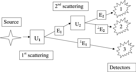
FIG. 1.: A history. Projector $E_{1}$ does not “reduce” states. Filters $U_{1}$ and $U_{2}$ are represented by unitary operators.

FIG. 2.: Averages of the three observables in the switching-function formulation. The dotted line shows the evolution of observable $\sigma_{x}$ associated with particle $\#2$ which is detected at $t=t_{2}=8$. Earlier detection of particle $\#1$ at $t_{1}=3.5$ does not influence particle $\#2$.

FIG. 3.: Averages of the three observables calculated in a Zeno-type way. Measurement at $t=t_{1}=3.5$ performed on particle $\#1$ nonlocally influences the behavior of particle $\#2$. As opposed to the plot from Fig. 2 the dotted line is modified at $t=3.5$. This is Gisin-type nonlocality.

REFERENCES

- [1] J. Polchinski, Phys. Rev. Lett. 66, 397 (1991).
- [2] T. W. Kibble, Comm. Math. Phys. 64, 73 (1978); Comm. Math. Phys. 65, 189 (1979).
- [3] S. Weinberg, Ann. Phys. (NY) 194, 336 (1989).
- [4] N. Gisin, Phys. Lett. A 143, 1 (1990); Helv. Phys. Acta 62, 363 (1989).
- [5] M. Czachor, unpublished preprints (1989,1990); Found. Phys. Lett. 4, 351 (1991).
- [6] S. Weinberg, Dreams of a Final Theory, Hutchinson (1993).
- [7] P. Bóna, preprint Ph10-91, Comenius University, Bratislava, 1991; Acta Phys. Slov. 50 (2000) 1, also available as math-ph/9909022.
- [8] T. F. Jordan, Ann. Phys. 225 (1993) 83.
- [9] M. Czachor, Phys. Rev. A 53 (1996) 1310.
- [10] M. Czachor, Phys. Rev. A 57 (1998) 4122.
- [11] M. Czachor, Phys. Lett. A 225 (1997) 1-12; Int. J. Theor. Phys. 38 (1999) 475-500.
- [12] M. Czachor and M. Kuna, Phys. Rev. A 58 (1998) 128.
- [13] S. B. Leble and M. Czachor,Phys. Rev. E 58 (1998) 7091.
- [14] M. Kuna, M. Czachor, and S. B. Leble, Phys. Lett. A 255 (1999) 42-48.
- [15] N. V. Ustinov, M. Czachor, M. Kuna, and S. B. Leble, Phys. Lett. A 279 (2001) 333-340.
- [16] N. V. Ustinov and M. Czachor, nlin.SI/0011013.
- [17] J. Cieśliński, University of Białystok, preprint IFT UwB/01/2001 (January 2001).
- [18] R. Cirelli, A. Mania, and L. Pizzocchero, J. Math. Phys. 31 (1990) 2891-2897; J. Math. Phys. 31 (1990) 2898-2903;
- [19] A. Ashtekar and T. A. Schilling, in On Einstein’s Path, A. Harvey, ed., Springer, Berlin, 1998.
- [20] D. C. Brody and L. P. Hughston, J. Geom. Phys. 38 (2001) 19-53.
- [21] H.-D. Doebner and G. A. Goldin, Phys. Lett. A 162 (1992) 397; J. Phys. A: Math. Gen. 27 (1994) 1771; Phys. Rev. A 54 (1996) 3764.
- [22] H.-D. Doebner, G. A. Goldin, and P. Nattermann, J. Math. Phys. 40 (1999) 49.
- [23] G. A. Goldin, Nonlinear Math. Phys. 4 (1997) 6.
- [24] E. C. Caparelli, V. V. Dodonov, and S. S. Mizrahi, Physica Scripta 58 (1998) 417.
- [25] G. A. Goldin, R. Menikoff, and D. H. Sharp, J. Math. Phys. 21 (1980), 650.
- [26] H.-D. Doebner and J. Tolar, in Symposium on Symmetries, Plenum, New York, 1980.
- [27] D. Schuch, K.-M. Chung, and H. Hartmann, J. Math. Phys. 24 (1983) 1672.
- [28] M. D. Kostin, J. Chem. Phys. 57 (1972) 3589.
- [29] I. Białynicki-Birula and J. Mycielski, Ann. Phys. 100 (1976) 62.
- [30] R. Haag and U. Bannier, Comm. Math. Phys. 60 (1978) 1.
- [31] F. Guerra and M. Pustella, Lett. Nuovo. Cim. 34 (1982) 351.
- [32] L. Stenflo, M. Y. Yu, and P. K. Shukla, Physica Scr. 40 (1989) 257.
- [33] P. C. Sabatier, Inverse Problems 6 (1990) L47.
- [34] B. A. Malomed and L. Stenflo, J. Phys. A: Math. Gen. 24 (1991) L1149.
- [35] N. E. Mavromatos and R. J. Szabo, Int. J. Mod. Phys. A 16 (2001) 209-250.
- [36] J. Ellis, N. E. Mavromatos, and D. V. Nanopoulos Phys. Rev. D 63 (2001) 024024.
- [37] M. Czachor and J. Naudts, Phys. Rev. E 59 (1999) R2497.
- [38] C. Tsallis, J. Stat. Phys. 52 (1988) 479-487.
- [39] C. Tsallis, R. S. Mendes, and A. R. Plastino, Physica A 280 (1998) 543-554.
- [40] N. Gisin and M. Rigo, J. Phys. A 28 (1995) 7375-7390.
- [41] G. A. Goldin, in Lie Theory and its Applications, ed. H.-D. Doebner, V. K. Dobrev and J. Hilgert, p. 210-221, World Scientific, Singapore, 1998.
- [42] B. Mielnik, quant-ph/0012041,
- [43] P. Bóna discussed this in detail in [7]. He distinguishes between “elementary mixtures” (in our terminology these are pure states on the Poisson manifold) and “barycenters” which are mixed in the standard sense. The main point is that generic states of subsystems are represented by reduced density matrices. The fact that they are not one dimensional projectors has an entirely quantum origin and has nothing to do with the so called “ignorance interpretation of quantum ensembles”. Similar oppinions on the ontological status of reduced density matrices were expressed in [44, 46, 47].
- [44] J. Anandan and Y. Aharonov, Found. Phys. Lett. 12 (1999) 571-578.
- [45] W. Lücke, in Nonlinear, deformed and Irreversible Quantum Systems, p. 140-154, H.-D. Doebner et al. eds., World Sientific, Singapore, 1995.
- [46] N. D. Mermin, Amer. J. Phys. 66 (1998) 753.
- [47] D. Aerts, Int. J. Theor. Phys. 39 (2000) 483.
- [48] R. Omnès, The Interpretation of Quantum Mechanics, Princeton University Press, Princeton, 1994.
- [49] B. Mielnik, Commun. Math. Phys. 15 (1969) 1; ibid. 31 (1974) 221.
- [50] J. B. Hartle, Amer. J. Phys. 36 (1968) 704.
- [51] E. Farhi, J. Goldstone, and S. Gutmann, Ann. Phys. 192 (1989) 368-382.
- [52] R. V. Hartley, Bell Syst. Tech. Jour. 7, 535 (1928).
- [53] C. E. Shannon, Bell Syst. Tech. Jour. 27, 379 (1948).
- [54] A. Rényi, in Selected Papers of Alfréd Rényi, Akadémiai Kiadó, Budapest (1976).