Decoherence and fluctuations in quantum interference experiments

A. Mariano, P. Facchi and S. Pascazio
 
Dipartimento di Fisica, Università di Bari
and Istituto Nazionale di Fisica Nucleare, Sezione di Bari
I-70126 Bari, Italy

Abstract

We analyze the notion of quantum coherence in an interference experiment. We let the phase shifts fluctuate according to a given statistical distribution and introduce a decoherence parameter, defined in terms of a generalized visibility of the interference pattern. One might naively expect that a particle ensemble suffers a greater loss of quantum coherence by interacting with an increasingly randomized distribution of shifts. As we shall see, this is not always true.

PACS: 03.75.Dg, 05.40.-a, 42.50.-p

1 Introduction

Decoherence is an interesting phenomenon and a topic that attracts widespread attention [1]. However, it is not easy to give a quantitative definition of decoherence [2]. All attempts at defining it always depend on the experimental configuration and on the authors’ taste. An interesting related quantity is the square of the density matrix [3]. This quantity enjoys interesting features [4], but also yields results which are at variance with naive expectations based on entropy [2]. We consider here an alternative, operational definition of decoherence, based on a fluctuation approach [5], and discuss its physical meaning by considering some examples.

2 Fluctuating phase shifter

Consider a Mach-Zender interferometer (MZI), with a phase shifter $\Delta$ in one of its two arms. If $|\psi_{\rm in}\rangle$ is the incoming state, the output state in the ordinary channel is

$$|\psi_{O}\rangle=\frac{1}{2}\left[1+e^{\frac{i}{\hbar}\hat{p}\Delta}\right]|\psi_{\rm in}\rangle\equiv\hat{O}(\Delta)|\psi_{\rm in}\rangle$$ (1)

or, in terms of the density matrix,

$$\hat{\rho}_{O}\equiv|\psi_{O}\rangle\langle\psi_{O}|=\hat{O}(\Delta)|\psi_{\rm in}\rangle\langle\psi_{\rm in}|\hat{O}(\Delta)^{\dagger}=\hat{O}(\Delta)\hat{\rho_{\rm in}}\hat{O}(\Delta)^{\dagger},$$ (2)

where $\hat{\rho}_{\rm in}$ is the density matrix of the incoming state. Suppose now that the shift $\Delta$ fluctuates according to a probability function $w(\Delta-\Delta_{0})$. The trace of the average density matrix is

$${\rm Tr}\;\overline{\hat{\rho}_{O}}={\rm Tr}\;\int\;d\Delta\;w(\Delta-\Delta_{0})\hat{O}(\Delta)\hat{\rho}_{\rm in}\hat{O}(\Delta)^{\dagger}={\rm Tr}\;\left(\hat{\rho}_{\rm in}\overline{\hat{O}(\Delta)^{\dagger}\hat{O}(\Delta)}\right)$$ (3)

and one obtains, after some algebra,

$$\overline{\hat{O}(\Delta)^{\dagger}\hat{O}(\Delta)}=\frac{1}{2}\left(1+\overline{\cos\frac{\hat{p}\Delta}{\hbar}}\right).$$ (4)

Consider now the Fourier transform of the probability density of the fluctuations

$$\Omega(\hat{p})\equiv\int\;d\Delta\;w(\Delta)e^{\frac{i}{\hbar}\hat{p}\Delta}=\int\;d\Delta\;w(\Delta)\cos\frac{\hat{p}\Delta}{\hbar}+i\int\;d\Delta\;w(\Delta)\sin\frac{\hat{p}\Delta}{\hbar}.$$ (5)

If we assume that the distribution of fluctuations is symmetric, $w(\Delta)=w(-\Delta)$, we get

$$\overline{\cos\frac{\hat{p}\Delta}{\hbar}}=\int\;d\Delta\;w(\Delta-\Delta_{0})\cos\frac{\hat{p}\Delta}{\hbar}=\cos\frac{\hat{p}\Delta_{0}}{\hbar}\;\Omega(\hat{p})$$ (6)

and (4) becomes

$$\overline{\hat{O}(\Delta)^{\dagger}\hat{O}(\Delta)}=\frac{1}{2}\left[1+\Omega(\hat{p})\cos\frac{\hat{p}\Delta_{0}}{\hbar}\right].$$ (7)

We notice that the same results are obtained with a different setup: consider a polarized neutron that interacts with a magnetic field perpendicular to its spin. Due to the longitudinal Stern-Gerlach effect, its wave packet is split into two components that travel with different speed and are therefore separated in space [6]. After a projection onto the initial spin state, the final state reads

$$|\psi_{\|}\rangle=\frac{1}{2}\left[e^{-\frac{i}{2\hbar}\hat{p}\Delta}+e^{\frac{i}{2\hbar}\hat{p}\Delta}\right]|\psi_{\rm in}\rangle\equiv\hat{O}^{\prime}(\Delta)|\psi_{\rm in}\rangle,$$ (8)

where $\Delta$ is in this case the spatial separation between the two wave packets corresponding to the two spin components. By averaging over $\Delta$ it is easy to show that one obtains again (7).

By plugging the average operator (7) into (3) one finally gets

$${\rm Tr}\;\overline{\hat{\rho}_{O}}=\frac{1}{2}\left[1+\left\langle\Omega(\hat{p})\cos\frac{\hat{p}\Delta_{0}}{\hbar}\right\rangle\right],$$ (9)

where $\langle\cdots\rangle$ denotes the expectation value over state $\rho_{\rm in}$. On the other hand, the momentum distribution is easily proved to read

$$P_{O}(p)=\langle p|\overline{\hat{\rho}_{O}}|p\rangle=\frac{1}{2}P_{\rm in}(p)\left[1+\Omega(p)\cos\frac{p\Delta_{0}}{\hbar}\right],$$ (10)

where

$$P_{\rm in}(p)=\langle p|\hat{\rho}_{\rm in}|p\rangle,\qquad\Omega(p)=\langle p|\Omega(\hat{p})|p\rangle.$$ (11)

We now introduce the visibility of the interference pattern

$${\cal V}(p)\equiv\frac{P_{O}(p)_{\rm MAX}-P_{O}(p)_{\rm min}}{P_{O}(p)_{\rm MAX}+P_{O}(p)_{\rm min}}=|\Omega(p)|,$$ (12)

where $P_{O}(p)_{\rm MAX}$ ($P_{O}(p)_{\rm min}$) is the maximum (minimum) value assumed by $P_{O}(p)$ when $\Delta_{0}$ varies. Notice that, according to this definition, the visibility is a function of momentum $p$. By using (5) and (11), one infers that the visibility is the modulus of the Fourier transform of the distribution of the shifts $\Delta$ and is therefore a quantity which is closely related to the physical features of the phase shifter. We now turn to a definition of decoherence.

3 Operational definition of decoherence

Consider the MZI introduced in the previous section. The relative frequency of particles detected in the ordinary channel is, by (9),

$${\cal N}_{O}(\Delta_{0})={\rm Tr}\;\overline{\hat{\rho}_{O}}=\frac{1}{2}\left[1+\left\langle\Omega(\hat{p})\cos\frac{\hat{p}\Delta_{0}}{\hbar}\right\rangle\right].$$ (13)

On the other hand, in the extraordinary ($E$) channel we get

$${\cal N}_{E}(\Delta_{0})={\rm Tr}\;\overline{\hat{\rho}_{E}}=\frac{1}{2}\left[1-\left\langle\Omega(\hat{p})\cos\frac{\hat{p}\Delta_{0}}{\hbar}\right\rangle\right].$$ (14)

(Note that ${\cal N}_{O}+{\cal N}_{E}=1$.) Their difference is

$${\cal N}_{O}(\Delta_{0})-{\cal N}_{E}(\Delta_{0})=\left\langle\Omega(\hat{p})\cos\frac{\hat{p}\Delta_{0}}{\hbar}\right\rangle=\int\;dp\;P_{\rm in}(p)\Omega(p)\cos\frac{p\Delta_{0}}{\hbar}$$ (15)

and one can define a generalized visibility

$${\cal V}=\max_{\Delta_{0}}|{\cal N}_{O}(\Delta_{0})-{\cal N}_{E}(\Delta_{0})|=\max_{\Delta_{0}}\left|\left\langle\Omega(\hat{p})\cos\frac{\hat{p}\Delta_{0}}{\hbar}\right\rangle\right|.$$ (16)

Notice that when $P_{\rm in}(p^{\prime})=\delta(p^{\prime}-p)$ (normalized monochromatic incoming state, to be improperly referred to as plane wave of momentum $p$), the generalized visibility reduces to the standard “local” visibility (12)

$${\cal V}=\max_{\Delta_{0}}\left|\int\;dp^{\prime}\;\delta(p^{\prime}-p)\Omega(p^{\prime})\cos\frac{p^{\prime}\Delta_{0}}{\hbar}\right|=\max_{\Delta_{0}}\left|\Omega(p)\;\cos\frac{p\Delta_{0}}{\hbar}\right|={\cal V}(p).$$ (17)

In general one gets

$${\cal V}\leq\max_{\Delta_{0}}\int\;dp\;P_{\rm in}(p)|\Omega(p)|\left|\cos\frac{p\Delta_{0}}{\hbar}\right|=\int\;dp\;P_{\rm in}(p){\cal V}(p)\leq 1.$$ (18)

The generalized visibility yields the maximum “distance” between the intensities ${\cal N}_{O}$ and ${\cal N}_{E}$ and is bounded by the “local” visibility averaged over the momentum distribution of the incoming state.

For a fluctuation-free phase shifter, i.e. for $w(\Delta)=\delta(\Delta)$, one obtains $\Omega(p)=1$ and the generalized visibility (16) becomes

$${\cal V}=\max_{\Delta_{0}}\left|\left\langle\cos\frac{\hat{p}\Delta_{0}}{\hbar}\right\rangle\right|=\max_{\Delta_{0}}\left|\int\;dp\;P_{\rm in}(p)\cos\frac{p\Delta_{0}}{\hbar}\right|=\int\;dp\;P_{\rm in}(p)=1,$$ (19)

for any incoming state $P_{\rm in}$. The example of an incoming Gaussian wave packet

$$P_{\rm in}(p)=\sqrt{\frac{2\delta^{2}}{\hbar^{2}\pi}}\exp\left(-\frac{2\delta^{2}}{\hbar^{2}}(p-p_{0})^{2}\right)$$ (20)

is shown in Figure 1, where it is apparent that ${\cal V}=1$.

Figure 1: ${\cal N}_{O}$ and ${\cal N}_{E}$ versus $k_{0}\Delta_{0}$ ($k_{0}=p_{0}/\hbar$) for an incoming Gaussian wave packet (20) with $k_{0}\delta=12$ and no fluctuations. The two intensities differ in phase by $\pi$ and their sum is 1. The generalized visibility (16) is 1.

If, on the other hand, the phase shifter fluctuates, the amplitude of the envelope function decreases and ${\cal V}<1$. We therefore give an operational definition of decoherence, by means of a decoherence parameter:

$$\varepsilon\equiv 1-{\cal V}=1-\max_{\Delta_{0}}\left|\left\langle\Omega(\hat{p})\cos\frac{\hat{p}\Delta_{0}}{\hbar}\right\rangle\right|.$$ (21)

Notice that, by Eq. (19), $\varepsilon=0$ for a fluctuation-free phase shifter (quantum coherence perfectly preserved), while $\varepsilon\to 1$ when the magnitude of the fluctuations increases, $\Omega(p)\to 0$ and the envelope function in Figure 1 squeezes out all oscillations, eventually yielding ${\cal N}_{O}(\Delta_{0})={\cal N}_{E}(\Delta_{0})$, independently of $\Delta_{0}$. Observe also that ${\cal V}$ and $\varepsilon$ are independent of the coherence of the initial state (namely, they do not depend on the off-diagonal terms of the density matrix). In this sense they measure the loss of quantum coherence.

4 Examples

Let us now look at some particular cases of fluctuations. Let the phases be distributed according to a Gaussian law with standard deviation $\sigma$

$$w(\Delta)=\frac{1}{\sqrt{2\pi\sigma^{2}}}\exp\left(-\frac{\Delta^{2}}{2\sigma^{2}}\right),$$ (22)

so that $\Omega(p)=\exp\left(-\frac{p^{2}\sigma^{2}}{2\hbar^{2}}\right)$ and the decoherence parameter reads

$$\varepsilon=1-\max_{\Delta_{0}}\left|\int\;dp\;P_{\rm in}(p)\exp\left(-\frac{p^{2}\sigma^{2}}{2\hbar^{2}}\right)\cos\left(\frac{p\Delta_{0}}{\hbar}\right)\right|.$$ (23)

For Gaussian wave packets (20) one gets

$$\varepsilon=1-\sqrt{\frac{\delta^{2}}{\delta^{2}+\sigma^{2}/4}}\exp\left(-\frac{\delta^{2}}{\delta^{2}+\sigma^{2}/4}\frac{\sigma^{2}k_{0}^{2}}{2}\right),$$ (24)

with $k_{0}=p_{0}/\hbar$. In this case, as it is clear from Figure 2, at fixed $\delta$

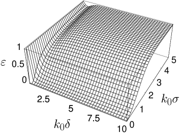
Figure 2: Decoherence parameter $\varepsilon$ (24) versus width $\delta$ of the Gaussian wave packet and standard deviation $\sigma$ of the fluctuating shifts ($k_{0}=p_{0}/\hbar$).

the decoherence parameter (21) increases with $\sigma$, although the details of its behavior are strongly dependent on the spatial width of the packet $\delta$. This behavior is in agreement with expectation: decoherence $\varepsilon$ increases with the magnitude of fluctuations $\sigma$.

For plane waves [$P_{\rm in}(p^{\prime})=\delta(p-p^{\prime})$]

$$\varepsilon_{k}=1-\max_{\Delta_{0}}\left|\int\;dp^{\prime}\;\delta(p-p^{\prime})e^{-\frac{p^{\prime 2}\sigma^{2}}{2\hbar^{2}}}\cos\left(\frac{p^{\prime}\Delta_{0}}{\hbar}\right)\right|=1-e^{-\frac{k^{2}\sigma^{2}}{2}},$$ (25)

with $k=p/\hbar$. This is shown in Figure 3(a) and can be obtained from (24) in the $\delta\to\infty$ limit. Notice that high momenta are more fragile against fluctuations [7].

Let now the phase shifts be distributed according to the law [2]

$$w(\Delta)=\frac{1}{\pi}\frac{1}{\sqrt{4\sigma^{2}-\Delta^{2}}}.$$ (26)

This is convenient from an experimental perspective and follows from a phase $\Delta(t)=2\sigma\sin t$, where $t$ (“time”) is a parameter, uniformly distributed between 0 and $2\pi$. From (11) and (5)

$$\Omega(p)=\int_{-2\sigma}^{2\sigma}\;\frac{d\Delta}{\pi}\frac{e^{i\frac{p\Delta}{\hbar}}}{\sqrt{4\sigma^{2}-\Delta^{2}}}=\int_{-\pi/2}^{\pi/2}\frac{dt}{\pi}\exp\left(i\frac{2p\sigma}{\hbar}\sin t\right)=J_{0}\left(\frac{2p\sigma}{\hbar}\right),$$ (27)

where $J_{0}$ is the Bessel function of order zero. The decoherence parameter (21) reads

$$\varepsilon=1-\max_{\Delta_{0}}\left|\int\;dp\;P_{\rm in}(p)J_{0}\left(\frac{2p\sigma}{\hbar}\right)\cos\left(\frac{p\Delta_{0}}{\hbar}\right)\right|$$ (28)

and for plane waves one obtains ($k=p/\hbar$)

$$\varepsilon_{k}=1-\max_{\Delta_{0}}\left|J_{0}\left(\frac{2p\sigma}{\hbar}\right)\cos\left(\frac{p\Delta_{0}}{\hbar}\right)\right|=1-|J_{0}(2k\sigma)|.$$ (29)

This function is shown in 3(b): observe that decoherence is not a monotonic function of the noise $\sigma$ in (26).

Figure 3: (a) Decoherence parameter $\varepsilon_{k}$ (25) versus $k\sigma$, for a plane wave interacting with a shifter fluctuating according to (22); (b) Decoherence parameter $\varepsilon_{k}$ (29) versus $k\sigma$, for a plane wave interacting with a shifter fluctuating according to (26).

A comparison between Figures 3(a) and 3(b) is interesting. In both cases one observes fragility at high momenta $p=\hbar k$. On the other hand, the behavior of decoherence in Figure 3(b) is somewhat anomalous and against naive expectation. For a given $k$, there are situations where decoherence $\varepsilon$ decreases by increasing the size of fluctuations $\sigma$. Note also that we are considering incoming plane waves, whence, according to (17), $\epsilon_{k}=1-{\cal V}(p)$ and the decoherence parameter is strictly related to the standard visibility of the interference pattern. Therefore, in the anomalous regions, one observes an increase in visibility by increasing the fluctuations of the phase shifter, a phenomenon similar to stochastic resonance [8]. However, this is true not only for plane waves, but also for narrow packets in momentum space.

These results are related to well known phenomena in the classical theory of partially coherent light [9], where the visibility is expressed as the Fourier transform of the spectral distribution of an incoherent source.

5 Conclusions

We have introduced and discussed a decoherence parameter defined in terms of a generalized visibility of the interference pattern in a double-slit experiment (MZI). Although the notion of visibility is not directly related to that of decoherence (see post-selection experiments [10]) our results corroborate the ideas expressed in [2] and make it obvious that the concept of “loss” of quantum mechanical coherence deserves clarification and additional investigation.

It would also be interesting to discuss analogies and differences with conceptual experiments in which decoherence is complemented by Welcher-Weg information [11].

References

• [1] D. Giulini et al, Decoherence and the Appearance of a Classical World in Quantum Theory (Springer, Berlin, 1996); M. Namiki, S. Pascazio and H. Nakazato, Decoherence and Quantum Measurements (World Scientific, Singapore, 1997).
• [2] P. Facchi, A. Mariano and S. Pascazio, Phys. Rev. A 63 (2001) 052108; Acta Phys. Slov. 49 (1999) 677; Physica B 276-278 (2000) 970.
• [3] S. Watanabe, Z. Phys. 113 (1939) 482; W.H. Furry, Boulder lectures in theoretical physics, Vol. 8A (University Colorado Press, 1966).
• [4] G. Manfredi and M.R. Feix, Phys. Rev. E 62 (2000) 4665.
• [5] M. Namiki and S. Pascazio, Phys. Lett. A 147 (1990) 430; Phys. Rev. A 44 (1991) 39; N. Kono, K. Machida, M. Namiki and S. Pascazio, Phys. Rev. A 54 (1996) 1064.
• [6] G. Badurek, H. Rauch, M. Suda and H. Weinfurter, Optics Comm. 179 (2000) 13.
• [7] H. Rauch and M. Suda, Physica B 241-243 (1998) 157; J. Appl. Phys. B 60 (1995) 181; H. Rauch, M. Suda and S. Pascazio, Physica B 267 (1999) 277.
• [8] R. Benzi, A. Sutera and A. Vulpiani, J. Phys. A 14 (1981) L453; R. Benzi, A. Sutera, G. Parisi and A. Vulpiani, SIAM (Soc. Ind. Appl. Math.) J. Appl. Math. 43 (1983) 565.
• [9] M. Born and E. Wolf: Principles of Optics, Cambridge University Press, Cambridge, 1999, Sec. 7.5.8.
• [10] H. Rauch, H. Wölwitsch, H. Kaiser, R. Clothier and S. A. Werner, Phys. Rev. A 53 (1996) 902.
• [11] M.O. Scully, B. Englert and J. Schwinger, Phys. Rev. A 40 (1989) 1775; B.G. Englert and J.A. Bergou, Opt. Comm. 179 (2000) 337; P. Facchi, A. Mariano and S. Pascazio, Mesoscopic interference, quant-ph/0105110.