Quantum Zeno phenomena: pulsed versus continuous measurement
P. Facchi and S. Pascazio
Dipartimento di Fisica, Università di Bari
and Istituto Nazionale di Fisica Nucleare, Sezione di Bari
I-70126 Bari, Italy
Abstract
The time evolution of an unstable quantum mechanical system coupled with an external measuring agent is investigated. According to the features of the interaction Hamiltonian, a quantum Zeno effect (hindered decay) or an inverse quantum Zeno effect (accelerated decay) can take place, depending on the response time of the apparatus. The transition between the two regimes is analyzed for both pulsed and continuous measurements.
PACS: 03.65.Xp
1 Quantum Zeno effect: fundamentals
Let be the total Hamiltonian of a quantum system. The survival probability of the system in state is
| (1) |
An elementary expansion yields a quadratic behavior at short times
| (2) |
where is called Zeno time. Observe that if one divides the Hamiltonian into a free and an interaction part , with and , the Zeno time reads and depends only on the off-diagonal part of the Hamiltonian.
We first consider “pulsed” measurements, as in the seminal approach [1]. The complementary notion of “continuous measurement” will be discussed in Sec. 4. Perform (instantaneous) measurements at time intervals (pulsed observation), in order to check whether the system is still in its initial state . The survival probability after the measurements reads
| (3) |
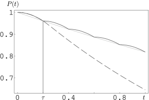
The (mathematical) limit is the quantum Zeno paradox: “A watched pot never boils”. For large (but finite) the evolution is slowed down (quantum Zeno effect). Indeed, the survival probability after pulsed measurements () is interpolated by an exponential law [2]
| (4) |
with an effective decay rate
| (5) |
For one gets , whence
| (6) |
increasingly frequent measurements hinder the evolution and tend to “freeze” it. The Zeno evolution is represented in Figure 1.
2 Unstable systems
Consider the spontaneous decay of state into state described by the Hamiltonian
| (7) |
with and , other commutators = 0. As is well known, the Fourier-Laplace transform of the survival amplitude in (1) is the expectation value of the resolvent
| (8) |
the Bromwich path B being a horizontal line constant in the half plane of convergence of the Fourier-Laplace transform (upper half plane). By performing Dyson’s resummation, the resolvent can be expressed in terms of the self-energy function
| (9) |
where is the form factor of the interaction (spectral density function).
If (which happens for sufficiently smooth form factors and small coupling), the resolvent is analytic in the whole complex plane cut along the positive real axis (continuous spectrum of ). On the other hand, there exists a pole located just below the branch cut in the second Riemann sheet, solution of the equation , being the determination of the self-energy function in the second sheet. The pole has a real and imaginary part given by
| (10) |
| (11) |
up to fourth order in the coupling constant. One recognizes the second-order energy shift and the celebrated Fermi “golden” rule [3]. The survival amplitude has the general form
| (12) |
where , being the branch-cut contribution. At intermediate times, the pole contribution dominates the evolution (Weisskopf-Wigner approximation [4]) and
| (13) |
where , the intersection of the asymptotic exponential with the axis, is the wave function renormalization. As is well known the exponential law is corrected by the cut contribution, which is responsible for a quadratic behavior at short times and a power law at long times.
3 Inverse quantum Zeno effect
Consider an unstable system with decay rate given by (11). By performing a single measurement at a sufficiently long time , when the exponential behavior is dominant, one infers from (4) that the effective decay rate is simply the natural (undisturbed) one
| (14) |
We now ask whether it is possible to find a finite time such that
| (15) |
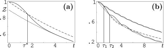
If such a time exists, then by performing measurements at time intervals the system decays according to its undisturbed decay rate , as if no measurements were performed. The related concept of “jump” time was considered in [5]. By (5) and (15) we get : the time is the intersection between the curves and . In the situation depicted in Figure 2(a) such a time exists: the full line is the survival probability and the dashed line the exponential [the dotted line is the asymptotic exponential , see (13)]. By looking at Figure 2(b) we realize that represents a transition time from a quantum Zeno to an inverse quantum Zeno regime [2]. Indeed
If exists, frequent measurements first accelerate decay (IZE) [6, 2], then, eventually, slow it down (QZE) when the frequency of measurements becomes larger than [2, 7]. Note that the existence of such a transition time is related to the value of the wave function renormalization : if a finite certainly exists [2] and the system exhibits both QZE and IZE, depending on the frequency of measurements. (This is the case considered in Figure 2.) The transition from a Zeno to an inverse Zeno regime has been recently confirmed in a beautiful experiment performed by Raizen’s group [7].
4 Pulsed versus continuous observation
We now introduce some alternative descriptions of a measurement process and discuss the notion of continuous measurement. This is to be contrasted with the idea of pulsed measurements, discussed in the previous sections and hinging upon von Neumann’s projections. We will show that the use of instantaneous pulsed measurements is not essential to obtain QZE [8, 9] or (possibly) IZE . We will provide a dynamical picture of the measurement process by introducing a Hamiltonian description of the interaction with the detector and show that the detector response time plays a role very similar to that of the period between measurements in the pulsed version [5]. We will also show that irreversibility is not an essential ingredient of this picture. By replacing an irreversible detector with an oscillating one, we show that QZE and IZE are a simple consequence of a strong interaction between the “observed” decaying system and an “observing” agent (the “detector”) which closely “looks” at the system [10].
4.1 Pulsed observation (period )
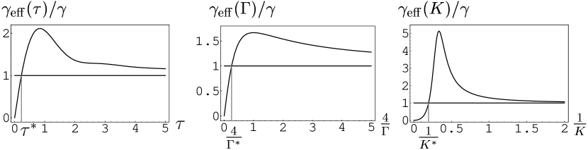
We start by considering pulsed measurements performed at time intervals . For simplicity we choose a Lorentzian form factor , from which an analytical expression of the survival amplitude can be easily obtained. (Notice that the Hamiltonian in this case is not lower bounded and one expects no deviations from exponential behavior at very large times.) We chose , and , so that , a finite exists and the system exhibits a QZE-IZE transition. The effective decay rate (5) is shown in the left frame of Figure 3 as a function of . Notice the linear behavior (6) for , with slope . Observe that for the chosen value of the parameters, the linear approximation (6) is valid well beyond the intersection and one gets . For the system decays faster, with a decay rate that first increases up to , then decreases and eventually relaxes to the natural decay rate according to (14).
4.2 Continuous observation (response time )
Let us consider now a continuous measurement process. This is accomplished, for instance, by adding to (7) the following interaction Hamiltonian
| (16) |
with , other commutators = 0. As soon as it becomes populated, state decays into state , with a decay rate . This yields a continuous monitoring of the decay process , with a response time . The presence of the interaction Hamiltonian (16) simply modifies the self-energy function in (9) as , whence, by (11),
| (17) |
The effective decay rate (17) is shown in the central frame of Figure 3 as a function of . The behavior is similar to that described in Sec. 4.1. For large values of one gets a linear behavior
| (18) |
which, when compared with (6), yields Schulman’s relation [5]. When , i.e. when the response of the apparatus is not very quick, the decay is accelerated (IZE). For one recovers the natural decay rate .
4.3 Continuous “Rabi” observation (response time )
The previous example is nothing but a more refined model of (the first stage of) a detection process than that given by the projection prescription. In this sense one might be led to think that irreversibility is a fundamental requisite for obtaining quantum Zeno effects: the observed system has to be coupled to a bona fide detector that irreversibly records its state. This expectation would be incorrect. In order to hinder (or accelerate) decay it is enough to introduce an external agent which couples differently to the initial state and to the “decay” products ( being the wave function of the system). In other words, one only needs an interaction which is able to distinguish whether the system is in its initial state or not: in this (very) loose sense the external agent can be viewed as a detector [10]. Let us illustrate this point by adding to (7) the following interaction Hamiltonian
| (19) |
which is probably the simplest way to include an external apparatus: as soon as state becomes populated it undergoes Rabi oscillations to state with Rabi frequency (detector response time ) [11]. The interaction modifies the self-energy function as , whence the effective decay rate reads [12]
| (20) |
and is shown in the right frame of Figure 3 as a function of . The behavior is similar to those previously described. For large values of one gets the behavior
| (21) |
Note, however, that this quadratic law, unlike the linear laws (6) and (18), is not generic, for it depends on the specific asymptotic behavior of the chosen form factor . As in the previous cases, when , i.e. when the response of the apparatus is not very quick, the decay is accelerated (IZE) and for the system eventually decays with the natural rate .
5 Conclusions
We have shown that the only requisite to obtain QZE is a coupling which is able to “pick out” the initial state of the system. For unstable systems this can also give rise to IZE. The recent experiment [7] has proved the existence of a transition from QZE to IZE in the case of pulsed measurements for a bona fide unstable system. It would be interesting to check the presence of such a transition also in the other cases envisaged in this paper (continuous and continuous Rabi observation).
References
- [1] B. Misra and E. C. G. Sudarshan, J. Math. Phys. 18 (1977) 756.
- [2] P. Facchi, H. Nakazato and S. Pascazio, Phys. Rev. Lett. 86 (2001) 2699.
- [3] E. Fermi, Rev. Mod. Phys. 4 (1932) 87.
- [4] G. Gamow, Z. Phys. 51 (1928) 204; V. Weisskopf and E.P. Wigner, Z. Phys. 63 (1930) 54; 65 (1930) 18; G. Breit and E.P. Wigner, Phys. Rev. 49 (1936) 519.
- [5] L.S. Schulman, J. Phys. A 30 (1997) L293; Phys. Rev. A 57 (1998) 1509.
- [6] A.G. Kofman and G. Kurizki, Nature 405 (2000) 546.
- [7] M.C. Fischer, B. Gutiérrez-Medina and M.G. Raizen, Observation of the Quantum Zeno and Anti-Zeno effects in an unstable system (2001), quant-ph/0104035.
- [8] A. Peres, Am. J. Phys. 48 (1980) 931; K. Kraus, Found. Phys. 11 (1981) 547.
- [9] A. Sudbery, Ann. Phys. 157 (1984) 512.
- [10] P. Facchi and S. Pascazio, in: Progress in Optics 42, Edited by E. Wolf, Elsevier Amsterdam, 2001; Quantum Zeno effects with “pulsed” and “continuous” measurements (2001) quant-ph/0101044.
- [11] A.D. Panov, Ann. Phys. 249 (1996) 1; Phys. Lett. A 260 (1999) 441.
- [12] E. Mihokova, S. Pascazio and L.S. Schulman, Phys. Rev. A 56 (1997) 25; S. Pascazio and P. Facchi, Acta Phys. Slov. 49 (1999) 557; P. Facchi and S. Pascazio, Phys. Rev. A 62 (2000) 023804.