1 Introduction

Entangled quantum states containing more than one photon on average have been of increasing interest. So, in continuous-variable quantum teleportation the entangled state shared by Alice and Bob is commonly assumed to be a Gaussian EPR-type state such as an infinitely squeezed two-mode squeezed vacuum (TMSV) [1], which then represents an entangled macroscopic state. Since entanglement is a nonclassical property, a strongly squeezed TMSV may be expected to be very instable; that is, strong entanglement degradation due to dissipative environments may be expected. This would of course have dramatic consequences for teleportation over reasonable distances of an arbitrary quantum state with sufficiently high fidelity.

The aim of the present paper is to investigate the problem of entanglement degradation in transmission of a TMSV through generically lossy optical systems such as fibers, with special emphasis on the ultimate limits in continuous-variable quantum teleportation. The necessarily existing interaction of the light with dissipative environments spoil the quantum-state purity, leaving behind a statistical mixture. Unfortunately, quantification of entanglement for mixed states in infinite-dimensional Hilbert spaces is yet impossible in practice. It typically involves minimizations over infinitely many parameters, as it is the case for the entropy of formation as well as for the distance to the set of all separable quantum states measured either by the relative entropy or Bures’ metric [2]. It is, however, possible to derive upper bounds on the entanglement content [3] by using the convexity property of the relative entropy.

For Gaussian states, however, an upper bound based on the distance to the set of separable Gaussian states can be derived, which is far better than the convexity bound. In particular, the entanglement degradation found in this way closely corresponds to the reduction of the fidelity of quantum teleportation. In this way, ultimate limits of quantum information transfer can be derived, which show that only a small fraction of the amount of quantum information that would be contained in an infinitely squeezed TMSV is really available in praxis.

2 Entanglement degradation

Let us consider the problem of entanglement degradation in transmission of light prepared in a TMSV state

$$|\mbox{TMSV}\rangle=\exp\!\left(\zeta^{\ast}\hat{a}_{1}\hat{a_{2}}-\zeta\hat{a}_{1}^{\dagger}\hat{a_{2}}^{\dagger}\right)|0,0\rangle=\sqrt{1-|q|^{2}}\,\sum\limits_{n=0}^{\infty}(-q)^{n}|n,n\rangle$$ (1)

($q$ $\!=$ $\!e^{i\phi}\tanh|\zeta|$, $\phi$ $\!=$ $\!\arg\zeta$) through absorbing fibers characterized by the transmission coefficients $T_{i}$ ($i$ $\!=$ $\!1,2$), which are given by the Lambert–Beer law of extinction,

$$|T_{i}|=e^{-l_{i}/l_{{\rm A}i}}$$ (2)

($l_{i}$, transmission length; $l_{{\rm A}i}$, absorption length). The quantum state of the transmitted field can be found by applying the formalism developed in [4, 5]. In the number basis it reads

$$\hat{\varrho}=(1-|q|^{2})\sum\limits_{m=0}^{\infty}\sum\limits_{k,l=0}^{\infty}\Big{[}K_{k,l,m}(c_{m}|m\!+\!k\rangle\langle k|+\mbox{H.c.})\otimes(d_{m}|m\!+\!l\rangle\langle l|+\mbox{H.c.})\Big{]},$$ (3)

where

$$c_{m} = (-q)^{m/2}T_{1}^{m}\left(1-{\textstyle\frac{1}{2}}\delta_{m0}\right),$$ (4)

$$d_{m} = (-q)^{m/2}T_{2}^{m}\left(1-{\textstyle\frac{1}{2}}\delta_{m0}\right),$$ (5)

and

$$K_{k,l,m}=\frac{\big{[}|q|^{2}(1\!-\!|T_{1}|^{2})(1\!-\!|T_{2}|^{2})\big{]}^{a}a!(a\!+\!m)!}{\sqrt{k!l!(k\!+\!m)!(l\!+\!m)!}(a\!-\!k)!(a\!-\!l)!}$$ (6)

$$\hskip 8.61108pt\times\left(\frac{|T_{1}|^{2}}{1-|T_{1}|^{2}}\right)^{k}\left(\frac{|T_{2}|^{2}}{1-|T_{2}|^{2}}\right)^{l}{}_{2}F_{1}\!\left[{a\!+\!1,\,a\!+\!m\!+\!1\atop|k\!-\!l|\!+\!1};\,|q|^{2}(1\!-\!|T_{1}|^{2})(1\!-\!|T_{2}|^{2})\right]$$

[$a$ $\!=$ $\!\max(k,l)$]. The state is a Gaussian state whose Wigner function reads

$$W(\alpha_{1},\alpha_{2})=\frac{4}{\pi^{2}\cal{N}}\exp\!\left[-2\bigl{(}C_{2}|\alpha_{1}|^{2}+C_{1}|\alpha_{2}|^{2}+S^{\ast}\alpha_{1}\alpha_{2}+S\alpha_{1}^{*}\alpha_{2}^{*}\bigr{)}\right],$$ (7)

where

$$S=\frac{e^{i\varphi}}{\cal{N}}\,T_{1}T_{2}\sinh|2\zeta|,$$ (8)

$$C_{i}=\frac{1}{\cal{N}}\left[1+|T_{i}|^{2}\left(\cosh|2\zeta|-1\right)\right],$$ (9)

$${\cal{N}}=1+\left(|T_{1}|^{2}+|T_{2}|^{2}-2|T_{1}|^{2}|T_{2}|^{2}\right)\left(\cosh|2\zeta|-1\right).$$ (10)

In Eqs. (3) and (7), the fibers are assumed to be in the ground state, which implies restriction to optical fields whose thermal excitation may be disregarded. Otherwise additional noise is introduced which enhance the entanglement degradation.

2.1 Entanglement estimate by pure state extraction

In order to quantify the entanglement content of a quantum state $\hat{\varrho}$, we make use of the relative entropy measuring the distance of the state to the set ${\cal S}$ of all separable states $\hat{\sigma}$ [2],

$$E(\hat{\varrho})=\min_{\hat{\sigma}\in{\cal S}}{\rm Tr}\big{[}\hat{\varrho}\big{(}\ln\hat{\varrho}-\ln\hat{\sigma}\big{)}\big{]}.$$ (11)

For pure states this measure reduces to the von Neumann entropy

$$E(\hat{\varrho})=S_{1(2)}=-{\rm Tr}\bigl{[}\hat{\varrho}_{1(2)}\ln\hat{\varrho}_{1(2)}\bigr{]},$$ (12)

where $\hat{\varrho}_{1(2)}$ denotes the (reduced) output density operator of mode $1(2)$, which is obtained by tracing $\hat{\varrho}$ with respect to mode $2(1)$. Thus,

$$E\big{(}|\mbox{TMSV}\rangle\big{)}=-\ln\big{(}1\!-\!|q|^{2}\big{)}-\frac{|q|^{2}}{1\!-\!|q|^{2}}\ln|q|^{2}.$$ (13)

Unfortunately, there is no closed solution of Eq. (11) for arbitrary mixed states. Nevertheless, upper bounds on the entanglement can be calculated, using the convexity of the relative entropy. When

$$\hat{\varrho}=\sum_{n}p_{n}\hat{\varrho}_{n},\quad\sum_{n}p_{n}=1$$ (14)

($p_{n}$ $\!\geq$ $\!0$), then $E(\hat{\varrho})$ satisfies the inequality

$$E(\hat{\varrho})\leq\sum_{n}p_{n}E(\hat{\varrho}_{n}).$$ (15)

If the $E(\hat{\varrho}_{n})$ are known, this inequality can be used to introduce an upper bound. Apart from pure states, it is known that when the quantum state has the Schmidt form,

$$\hat{\varrho}=\sum\limits_{n,m}C_{n,m}|\phi_{n},\psi_{n}\rangle\langle\phi_{m},\psi_{m}|,$$ (16)

then the amount of entanglement measured by the relative entropy is given by [6, 7]

$$E(\hat{\varrho})=-\sum_{n}C_{n,n}\ln C_{n,n}-S(\hat{\varrho}).$$ (17)

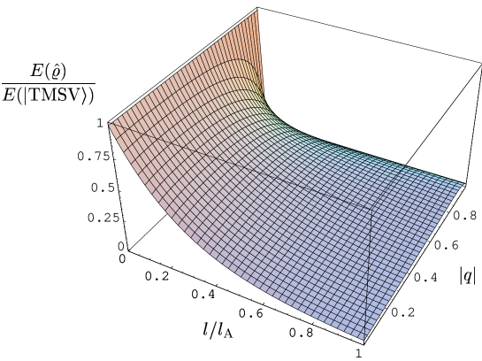
Figure 1: Estimate of the entanglement, Eq. (20), observed after transmission of a TMSV through absorbing fibers ($T_{1}$ $\!=$ $\!T_{2}$) as a function of the squeezing parameter $|q|$ $\!=$ $\!\sinh|\zeta|$ and the transmission length $l$.

2.1.1 Extraction of a single pure state

Since, by Eqs. (3) – (6), for low squeezing only a few matrix elements are excited which were not contained in the original Fock expansion (1), we can forget about the entanglement that could be present in the newly excited elements and treat them as contributions to the separable states only. The inseparable state relevant for entanglement might then be estimated to be the pure state

$$\sqrt{1-\lambda}\,|\Psi\rangle=\sqrt{\frac{1-|q|^{2}}{K_{000}}}\sum\limits_{n=0}^{\infty}K_{00n}c_{n}d_{n}|n,n\rangle.$$ (18)

It has the properties that only matrix elements of the same type as in the input TMSV state occur and the coefficients of the matrix elements $|0,0\rangle$ $\!\leftrightarrow$ $\!|n,n\rangle$ are met exactly, i.e.,

$$(1-\lambda)\langle 0,0|\Psi\rangle\langle\Psi|n,n\rangle=\langle 0,0|\hat{\varrho}|n,n\rangle.$$ (19)

In this approximation, the calculation of the entanglement of the mixed output quantum state reduces to the determination of the entanglement of a pure state [5]:

$$E(\hat{\varrho})\approx(1-\lambda)\,E(|\Psi\rangle)$$ (20)

$$\hskip 8.61108pt=\frac{1\!-\!x}{(1\!-\!x)^{2}\!-\!y}\,\ln\!\left[\frac{1\!-\!x}{(1\!-\!x)^{2}\!-\!y}\right]+\,\frac{(1\!-\!x)\{[y\!+\!(1\!-\!x)^{2}]\ln(1\!-\!x)\!-\!y\ln y\}}{[y\!-\!(1\!\!-x)^{2}]^{2}}\,,$$

where

$$x=|q|^{2}(1-|T_{1}|^{2})(1-|T_{2}|^{2}),$$ (21)

$$y=|qT_{1}T_{2}|^{2}.$$ (22)

In Fig. 1, the estimate of entanglement as given by Eq. (20) is plotted as a function of the transmission length and the strength of initial squeezing for $T_{1}$ $\!=$ $\!T_{2}$ $\!=$ $\!T$.

2.1.2 Upper bound of entanglement

As already mentioned, the estimate given by Eq. (20) is valid for low squeezing. Higher squeezing amounts to more excited density matrix elements and Eq. (20) might become wrong. Moreover, we cannot even infer it to be a bound in any sense since no inequality has been involved. A possible way out would be to extract successively more and more pure states from Eq. (3). But instead, let us follow Ref. [3], writing the density operator (3) as the convex sum of density operators in Schmidt decomposition,

$$\hat{\varrho}=\sum\limits_{k,l=0}^{\infty}\bigg{\{}A_{k,l}|k,k\rangle\langle l,l|+\sum\limits_{m=1}^{\infty}B_{k,l,m}|k\!+\!m,k\rangle\langle l\!+\!m,l|+\sum\limits_{m=1}^{\infty}C_{k,l,m}|k,k\!+\!m\rangle\langle l,l\!+\!m|\bigg{\}},$$ (23)

and applying the inequality (15) together with Eq. (17). The result is illustrated in Fig. 2.

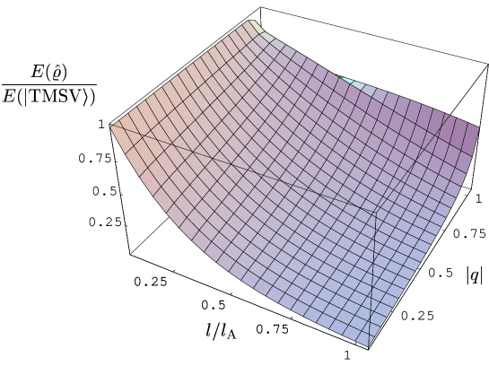
Figure 2: Upper bound on the entanglement degradation of a TMSV transmitted through absorbing fibers ($T_{1}$ $\!=$ $\!T_{2}$) as a function of the squeezing parameter $|q|$ $\!=$ $\!\sinh|\zeta|$ and the transmission length $l$. In the numerical calculation, at most 30 photons per mode have been taken into account which is obviously not sufficient for higher squeezing when higher photon-number states are excited.

From general arguments one would expect the entanglement to decrease faster the more squeezing one puts into the TMSV, because stronger squeezing is equivalent to saying the state is more macroscopically non-classical and quantum correlations should be destroyed faster. As an example, one would have to look at the entanglement degradation of an $n$-photon Bell-type state $|\Psi^{\pm}_{n}\rangle$, $E[\hat{\varrho}(|\Psi^{\pm}_{n}\rangle)]$ $\!\leq$ $\!|T|^{2n}\ln 2$ [8]. Since the transmission coefficient $T$ decreases exponentially with the transmission length, entanglement decreases even faster. Note that similar arguments also hold for the destruction of the interference pattern of a cat-like state $\sim|\alpha\rangle+|-\alpha\rangle$ when it is transmitted, e.g., through a beam splitter. It is well known that the two peaks (in the $j$th output channel) decay as $|T_{j}|^{2}$, whereas the quantum interference decays as $|T_{j}|^{2}\exp[-2|\alpha|^{2}(1$ $\!-$ $\!|T_{j}|^{2})]$.

The upper bound on the entanglement as calculated above seems to suggest that the entanglement degradation is simply exponential with the transmission length for essentially all (initial) squeezing parameters, which would make the TMSV a good candidate for a robust entangled quantum state. But this is a fallacy. The higher the squeezing, the more density matrix elements are excited, and the more terms appear, according to Eq. (23), in the convex sum (15). Equivalently, more and more separable states are mixed into the full quantum state. By that, the inequality gets more inadequate. We would thus conclude that the upper bound proposed in [3] is insufficient.

2.2 Distance to separable Gaussian states

The methods of computing entanglement estimates and bounds as considered in the preceding sections are based on Fock-state expansions. In practice they are typically restricted to situations where only a few quanta of the overall system (consisting of the field and the device) are excited, otherwise the calculation even of the matrix elements becomes arduous. Here we will focus on another way of computing the relative entropy, which will also enable us to give an essentially better bound on the entanglement.

Since it is close to impossible to compute the distance of a Gaussian state to the set of all separable states we restrict ourselves to separable Gaussian states. A quantum state is commonly called Gaussian if its Wigner function is Gaussian. The density operator of such a state can be written in exponential form of

$$\hat{\sigma}={\cal N}_{\sigma}\exp\!\left[-\left(\hat{a}^{\dagger}\,\hat{a}\right){\bf M}_{\sigma}{\hat{a}\choose\hat{a}^{\dagger}}\right],$$ (24)

where ${\bf M}_{\sigma}$ is a Hermitian matrix, which can be assumed to give a symmetrically ordered density operator, and ${\cal N}_{\sigma}$ is a suitable normalization factor. Here and in the following we restrict ourselves to Gaussian states with zero mean. Since coherent displacements, being local unitary transformations, do not influence entanglement, they can be disregarded.

The relative entropy (11) can now be written as

$$E\big{(}\hat{\varrho}\big{)}={\rm Tr}\left(\hat{\varrho}\ln\hat{\varrho}\right)-\min_{\hat{\sigma}\in{\cal S}}{\rm Tr}\left\{\hat{\varrho}\left[\ln{\cal N}_{\sigma}-\left(\hat{a}^{\dagger}\,\hat{a}\right){\bf M}_{\sigma}{\hat{a}\choose\hat{a}^{\dagger}}\right]\right\}.$$ (25)

Since we have chosen the density operator $\hat{\sigma}$ to be symmetrically ordered, the last term in Eq. (25) is nothing but a sum of (weighted) symmetrically ordered expectation values $\langle\hat{a}^{\dagger m}\hat{a}^{n}\rangle_{s=0}$ ($m$ $\!+$ $\!n$ $\!=$ $\!2$). Equation (25) can equivalently be given in terms of the matrix ${\bf D}_{\varrho}$ in the exponential of the characteristic function of the Wigner function as

$$E\big{(}\hat{\varrho}\big{)}={\rm Tr}\left(\hat{\varrho}\ln\hat{\varrho}\right)+\min_{\hat{\sigma}\in{\cal S}}\!\left[\textstyle\frac{1}{2}{\rm Tr}\left({\bf M}_{\sigma}{\bf D}_{\varrho}\right)-\ln{\cal N}_{\sigma}\right].$$ (26)

The matrix ${\bf D}_{\varrho}$ is unitarily equivalent to the variance matrix ${\bf V}$. For a Gaussian distribution with zero mean the elements of the variance matrix are defined by the (symmetrically ordered) correlations of the quadrature components $\hat{x}_{1},\hat{p}_{1},\hat{x}_{2},\hat{p}_{2}$. The variance matrix of any Gaussian state can be brought to the generic form

$${\bf V}=\left(\begin{array}[]{cccc}x&0&z_{1}&0\\ 0&x&0&z_{2}\\ z_{1}&0&y&0\\ 0&z_{2}&0&y\end{array}\right)$$ (27)

by local Sp(2,$\mathbb{R}$)$\otimes$Sp(2,$\mathbb{R}$) transformations [9], so that we can restrict our attention to that case. Separability requires that [9, 10]

$$4(xy-z_{1}^{2})(xy-z_{2}^{2})\geq(x^{2}+y^{2})+2|z_{1}z_{2}|-\textstyle\frac{1}{4}\,.$$ (28)

From Eq. (7) [together with Eqs. (8) and (9)] it follows that we may set

$$x={\textstyle\frac{1}{2}}{\cal N}C_{1},\quad y={\textstyle\frac{1}{2}}{\cal N}C_{2},$$ (29)

$$z_{1}=-z_{2}={\textstyle\frac{1}{2}}{\cal N}|S|.$$ (30)

Combining Eqs. (28) – (30), it is not difficult to prove that the boundary between separability and inseparability is reached for $T_{1}$ $\!=$ $\!T_{2}$ $\!=$ $\!0$; that is, for infinite transmission length [5, 10, 11]. Clearly, this tells us nothing about the entanglement degradation and the amount of entanglement that is really available for chosen transmission lengths.

In order to obtain a measure of the entanglement degradation, we therefore compute the distance of the quantum state of the transmitted light to the set of all Gaussian states satisfying the equality in (28), since they just represent the boundary between separability and inseparability. These states are completely specified by only three real parameters [one of the parameters in the equality in (28) can be computed by the other three]. With regard to Eq. (26), minimization is thus only performed in a three-dimensional parameter space. Results of the numerical analysis are shown in Fig. 3. It is clearly seen that the entanglement content (relative to the entanglement in the initial TMSV) decreases noticeably faster for larger squeezing, or equivalently, for higher mean photon number [the relation between the mean photon number $\bar{n}$ and the squeezing parameters being $\bar{n}$ $\!=$ $\!\sinh^{2}|\zeta|$ $\!=$ $\!|q|^{2}/(1$ $\!-$ $\!|q|^{2})$].

Figure 3: Entanglement degradation of a TMSV transmitted through absorbing fibers ($T_{1}$ $\!=$ $\!T_{2}$) as a function of the transmission length $l$ for the (initial) mean photon numbers $\bar{n}$ $\!=$ $1$ ($|q|$ $\!\simeq$ $\!0.7071$) (topmost curve), $\bar{n}$ $\!=$ $10$ ($|q|$ $\!\simeq$ $\!0.9535$), $\bar{n}$ $\!=$ $10^{2}$ ($|q|$ $\!\simeq$ $\!0.9950$), and $\bar{n}$ $\!=$ $10^{3}$ ($|q|$ $\!\simeq$ $\!0.9995$) (lowest curve).

2.3 Comparison of the methods

In Fig. 4 the entanglement degradation as calculated in Section 2.2 is compared with the estimate obtained in Section 2.1.1 and the bound obtained in Section 2.1.2. The figure reveals that the distance of the output state to the separable Gaussian states (lower curve) is much smaller than it might be expected from the bound on the entanglement (upper curve) calculated by applying the inequality (15) [together with Eqs. (17)] to Eq. (23), as well as the estimate (middle curve) derived by extracting a single pure state according to Eq. (20). Note that the entanglement of the single pure state (18) comes closest to the distance of the actual state to the separable Gaussian states, whereas the convex sum (23) of density operators in Schmidt decomposition can give much higher values. Both methods, however, overestimate the entanglement. Since with increasing mean photon number the convex sum contains more and more terms, the bound gets worse [and substantially slower on the computer, whereas computation of the distance measure (26) does not depend on it].

Figure 4: Comparison of the upper bound on entanglement (upper curve) according to Fig. 2, the entanglement estimate (middle curve) according to Fig. 1, and the distance measure (lower curve) according to Fig. 3 for the mean photon number $\bar{n}$ $\!=$ $1$ ($|q|$ $\!\simeq$ $\!0.7071$).

Thus, in our view, the distance to the separable Gaussian states should be the measure of choice for determining the entanglement degradation of entangled Gaussian states. Nevertheless, it should be pointed out that the distance to separable Gaussian states has been considered and not the distance to all separable states. We have no proof yet, that there does not exist an inseparable non-Gaussian state which is closer than the closest Gaussian state.

3 Quantum teleportation

It is very instructive to know how much entanglement is available after transmission of the TMSV through the fibers. Examples of the (maximally) available entanglement for different transmission lengths are shown in Fig. 5. One observes that a chosen transmission length allows only for transport of a certain amount of entanglement. The saturation value, which is quite independent of the value of the input entanglement, drastically decreases with increasing transmission length (compare the upper curve with the two lower curves in the figure). This has dramatic consequences for applications in quantum information processing such as continuous-variable teleportation, where a highly squeezed TMSV is required in order to teleport an arbitrary quantum state with sufficiently high fidelity. Even if the input TMSV would be infinitely squeezed, the available (low) saturation value of entanglement principally prevents one from high-fidelity teleportation of arbitrary quantum states over finite distances.

Figure 5: Available entanglement after transmission of a TMSV through absorbing fibers ($T_{1}$ $\!=$ $\!T_{2}$) as a function of the squeezing parameter $|\zeta|$ for various transmission lengths $l$ [$l$ $\!=$ $\!0$ (topmost curve), $l$ $\!=$ $\!10^{-2}\,l_{A}$ (middle curve), $l$ $\!=$ $\!10^{-1}\,l_{A}$ (lowest curve)]. For $|\zeta|$ $\!<$ $\!0.5$ and $l/l_{A}$ $\!<$ $\!10^{-2}$, the numerical accuracy of the values of $E(\hat{\varrho})$ decreases due to the low accuracy in the eigenvector computation.

3.1 The teleported state

Let us briefly repeat the main stages of teleportation (Fig. 6). If $W_{\rm in}(\gamma)$ is the Wigner function of the signal-mode quantum state that is desired to be teleported and $W(\alpha,\beta)$ is, according to Eq. (7) ($\alpha_{1}$ $\!=$ $\!\alpha$, $\alpha_{2}$ $\!=$ $\!\beta$), the Wigner function of the entangled state that is shared by Alice and Bob, the Wigner function of the (three-mode) overall system then reads

$$W(\gamma,\alpha,\beta)=W_{\rm in}(\gamma)\,W(\alpha,\beta).$$ (31)

After combination of the signal mode and Alice’s mode of the entangled two-mode system through a 50%:50% (lossless) beam splitter the Wigner function changes to

$$W(\mu,\nu,\beta)=W_{\rm in}\!\left(\frac{\mu-\nu}{\sqrt{2}}\right)W\!\left(\frac{\mu+\nu}{\sqrt{2}},\beta\right).$$ (32)

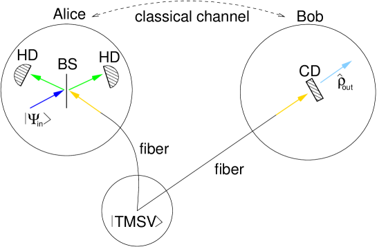
Figure 6: Scheme of teleportation (BS, beam splitter; HD, homodyne detection; HD, coherent displacement).

Measurement of the real part of $\mu$, $\mu_{\rm R}$, and the imaginary part of $\nu$, $\nu_{\rm I}$, then prepares Bob’s mode in a quantum state whose Wigner function is given by

$$W(\beta|\mu_{\rm R},\nu_{\rm I})=\frac{1}{P(\mu_{\rm R},\nu_{\rm I})}\int d\nu_{\rm R}\int d\mu_{\rm I}\,W_{\rm in}\!\left(\frac{\mu-\nu}{\sqrt{2}}\right)W\!\left(\frac{\mu+\nu}{\sqrt{2}},\beta\right),$$ (33)

where

$$P(\mu_{\rm R},\nu_{\rm I})=\int d\nu_{\rm R}\int d\mu_{\rm I}\int d^{2}\beta\,W(\mu,\nu,\beta)$$ (34)

is the probability density of measuring $\mu_{\rm R}$ and $\nu_{\rm I}$. Introducuing the complex variables

$$\gamma=\left(\mu-\nu\right)/\sqrt{2},\quad\gamma^{\prime}=\sqrt{2}\left(\mu_{\rm R}-i\nu_{\rm I}\right),$$ (35)

we may rewrite Eq. (33) as

$$W(\beta|\gamma^{\prime})=\frac{1}{P(\gamma^{\prime})}\int d^{2}\gamma\,W_{\rm in}(\gamma)\,W({\gamma^{\prime}}^{*}\!-\!{\gamma}^{*},\beta)$$ (36)

[$P(\mu_{\rm R},\nu_{\rm I})/2$ $\!\to$ $\!P(\gamma^{\prime})$].

Depending upon the result of Alice’s measurement, Bob now coherently displaces the quantum state of his mode in order to generate a quantum state whose Wigner function is $W(\beta$ $\!-$ $\!\Delta(\gamma^{\prime})|\gamma^{\prime})$. If we are not interested in the one or the other measurement result, we may average over all measurement results to obtain the teleported quantum state on average:

$$W_{\rm out}(\beta) = \int d^{2}\gamma^{\prime}\,P(\gamma^{\prime})\,W\!\left(\beta-\Delta(\gamma^{\prime})|\gamma^{\prime}\right)$$ (37)

$$= \int d^{2}\gamma\,W_{\rm in}(\gamma)\!\int d^{2}\gamma^{\prime}\,W\!\left({\gamma^{\prime}}^{*}\!-\!{\gamma}^{*},\beta\!-\!\Delta(\gamma^{\prime})\right).$$

Let us assume that the quantum state to be teleported is pure, $\hat{\varrho}_{\rm in}$ $\!=$ $\!|\psi_{\rm in}\rangle\langle\psi_{\rm in}|$. A measure of how close to it is the (mixed) output quantum state $\hat{\varrho}_{\rm out}$ is the teleportation fidelity

$$F=\langle\psi_{\rm in}|\hat{\varrho}_{\rm out}|\psi_{\rm in}\rangle\,,$$ (38)

which can be rewritten as the overlap of the Wigner functions:

$$F=\pi\int d^{2}\beta\,W_{\rm in}(\beta)W_{\rm out}(\beta).$$ (39)

Perfect teleportation implies unit fidelity; that is, perfect overlap of the Wigner functions of the input and the output quantum state. Clearly, losses prevent one from realizing this case, so that the really observed fidelity is always less than unity. Thus, the task is to choose the scheme-inherent parameters such that the fidelity is maximized.

3.2 Choice of the displacement

An important parameter that must be specified is the displacement $\beta$ $\!\to$ $\!\beta$ $\!-$ $\!\Delta(\gamma^{\prime})$, which has to be performed by Bob after Alice’s measurement. For this purpose, we substitute Eq. (7) into Eq. (36) to obtain, on using the relation $C_{1}C_{2}$ $\!-$ $\!|S|^{2}$ $\!=$ $\!{\cal N}^{-1}$,

$$W(\beta|\gamma^{\prime})=\frac{1}{P(\gamma^{\prime})}\frac{2}{\pi{C_{2}\cal{N}}}\,\exp\!\left(-\frac{2}{C_{2}\cal{N}}|\beta|^{2}\right)$$ (40)

$$\hskip 8.61108pt\times\int d^{2}\gamma\,\frac{2C_{2}}{\pi}\,\exp\!\left(\!-2C_{2}\left|\gamma^{\prime}\!-\!\gamma\!+\!\frac{S^{*}}{C_{2}}\beta\right|^{2}\right)W_{\rm in}(\gamma).$$

Here and in the following we restrict our attention to optical fields whose thermal excitation may be disregarded ($n_{{\rm th}\,i}$ $\!\approx$ $\!0$). From Eqs. (9) and (10) it follows that, for not too small values of the (initial) squeezing parameter $|\zeta|$, the variance of the Gaussian in the first line of Eq. (40), $C_{2}{\cal{N}}/4$, increases with $|\zeta|$ as $e^{2|\zeta|}|T_{2}|^{2}/8$, whereas the variance of the Gaussian in the integral in the second line, $1/(4C_{2})$, rapidly approaches the (finite) limit ($T_{2}$ $\!\not=$ $\!0$)

$$\sigma_{\infty}=\lim_{|\zeta|\to\infty}\frac{1}{4C_{2}}=\frac{|T_{1}|^{2}+|T_{2}|^{2}-2|T_{1}T_{2}|^{2}}{4|T_{2}|^{2}}\,.$$ (41)

Thus, Bob’s mode is prepared (after Alice’s measurement) in a quantum state that is obtained, roughly speaking, from the input quantum state by shifting the Wigner function according to $\gamma$ $\!\to$ $\!\gamma^{\prime}$ $\!+$ $\!\beta S^{*}/C_{2}$ and smearing it over an area whose linear extension is given by $2\sqrt{\sigma_{\infty}}$. It is therefore expected that the best what Bob can do is to perform a displacement with

$$\Delta(\gamma^{\prime})=e^{i\tilde{\varphi}}\lambda\gamma^{\prime},$$ (42)

where $\tilde{\varphi}$ $\!=$ $\!\varphi$ $\!+$ $\!\arg T_{1}$ $\!+$ $\arg T_{2}$ and

$$\lambda=\lim_{|\zeta|\to\infty}\frac{C_{2}}{|S|}=\left|\frac{T_{2}}{T_{1}}\right|.$$ (43)

Substitution of the expression (42) into Eq. (37) yields

$$W_{\rm out}(\beta e^{i\tilde{\varphi}})=\frac{1}{2\pi\sigma\lambda^{2}}\int d^{2}\gamma\,W_{\rm in}(\gamma)\exp\!\left(-\frac{|\gamma-\beta/\lambda|^{2}}{2\sigma}\right)\!,$$ (44)

where

$$\sigma=\frac{\cal{N}}{4\lambda^{2}}\left(C_{2}+\lambda^{2}C_{1}-2\lambda|S|\right).$$ (45)

Note that $\lim_{|\zeta|\to\infty}\sigma$ $\!=$ $\!\sigma_{\infty}$.

Clearly, even for arbitrarily large squeezing, i.e, $|\zeta|$ $\!\to$ $\infty$, and thus arbitrarily large entanglement, the input quantum state cannot be scanned precisely due to the unavoidable losses, which drastically reduce, in agreement with the entanglement degradation calculated in Section 2, the amount of information that can be transferred nonclassically from Alice to Bob. Let $\delta_{W}$ be a measure of the (smallest) scale on which the Wigner function of the signal-mode state, $W_{\rm in}(\gamma)$, typically changes. Teleportation then requires, apart from the scaling by $\lambda$, that the condition

$$\sigma_{\infty}\ll\delta_{W}^{2}$$ (46)

is satisfied. Otherwise, essential information about the finer points of the quantum state are lost. For given $\delta_{W}$, the condition (46) can be used in order to determine the ultimate limits of teleportation, such as the maximally possible distance between Alice and Bob. In this context, the question of the optimal position of the source of the TMSV arises. Needless to say, that all the results are highly state-dependent. Let us study the problem for squeezed states and Fock states in more detail.

3.3 Squeezed states

The Wigner function of a squeezed coherent state can be given in the form of

$$W_{\rm in}(\gamma)=\frac{N_{\rm in}}{\pi}\,\exp\!\left[-A_{\rm in}|\gamma|^{2}-B_{\rm in}\left(\gamma^{2}+\gamma^{\ast 2}\right)+C_{\rm in}^{\ast}\gamma+C_{\rm in}\gamma^{\ast}\right],$$ (47)

where

$$N_{\rm in}=2\exp\!\left[-2|\alpha_{0}|^{2}\cosh\!\left(2\zeta_{0}\right)-\left(\alpha_{0}^{2}+\alpha_{0}^{*2}\right)\sinh\!\left(2\zeta_{0}\right)\right],$$ (48)

$$A_{\rm in}=2\cosh(2\zeta_{0}),$$ (49)

$$B_{\rm in}=\sinh(2\zeta_{0}),$$ (50)

$$C_{\rm in}=2\left[\alpha_{0}\cosh\!\left(2\zeta_{0}\right)+\alpha_{0}^{*}\sinh\!\left(2\zeta_{0}\right)\right].$$ (51)

Here, $\alpha_{0}$ is the coherent amplitude and $\zeta_{0}$ is the squeezing parameter which is chosen to be real. Substituting Eq. (47) [together with Eqs. (48) – (51)] into Eq. (44), we derive

$$W_{\rm out}(\beta)=\frac{N_{\rm out}}{\pi}\,\exp\!\left[-A_{\rm out}|\beta|^{2}-B_{\rm out}\left(\beta^{2}+\beta^{\ast 2}\right)+C_{\rm out}^{\ast}\beta+C_{\rm out}\beta^{\ast}\right],$$ (52)

where

$$N_{\rm out}=\frac{2\exp\!\left\{-\displaystyle\frac{2|\alpha_{0}|^{2}\left[\cosh\!\left(2\zeta_{0}\right)+4\sigma\right]+\left(\alpha_{0}^{2}+\alpha_{0}^{*2}\right)\sinh\!\left(2\zeta_{0}\right)}{1+8\sigma\cosh\!\left(2\zeta_{0}\right)+16\sigma^{2}}\right\}}{\lambda^{2}\sqrt{1+8\sigma\cosh\!\left(2\zeta_{0}\right)+16\sigma^{2}}}\,,$$ (53)

$$A_{\rm out}=\frac{2\left[\cosh\!\left(2\zeta_{0}\right)+4\sigma\right]}{\lambda^{2}\left[1+8\sigma\cosh\!\left(2\zeta_{0}\right)+16\sigma^{2}\right]}\,,$$ (54)

$$B_{\rm out}=\frac{\sinh\!\left(2\zeta_{0}\right)}{\lambda^{2}\left[1+8\sigma\cosh\!\left(2\zeta_{0}\right)+16\sigma^{2}\right]}\,,$$ (55)

$$C_{\rm out}=2\frac{\alpha_{0}\left[\cosh\!\left(2\zeta_{0}\right)+4\sigma\right]+\alpha_{0}^{*}\sinh\!\left(2\zeta_{0}\right)}{\lambda\left[1+8\sigma\cosh\!\left(2\zeta_{0}\right)+16\sigma^{2}\right]}$$ (56)

($\tilde{\varphi}$ $\!=$ $\!0$). Combining Eqs. (39), (47) – (51), and (52) – (56), we arrive at the following expression for the fidelity

$$F\equiv F(\zeta_{0},\alpha_{0})=F(\zeta_{0})\exp\!\left\{-\frac{(1-\lambda)^{2}}{2}\left[\frac{\left(\alpha_{0}+\alpha_{0}^{*}\right)^{2}e^{2\zeta_{0}}}{1+\lambda^{2}\left(1+4e^{2\zeta_{0}}\sigma\right)}-\frac{\left(\alpha_{0}-\alpha_{0}^{*}\right)^{2}}{\left(1+\lambda^{2}\right)e^{2\zeta_{0}}+4\lambda^{2}\sigma}\right]\right\},$$ (57)

where

$$F(\zeta_{0})=\frac{2}{\sqrt{1\!+\!2\lambda^{2}\!+\!\lambda^{4}\left(1\!+\!16\sigma^{2}\right)\!+\!8\lambda^{2}\left(1\!+\!\lambda^{2}\right)\sigma\cosh\!\left(2\zeta_{0}\right)}}$$ (58)

is the fidelity for teleporting the squeezed vacuum.

From Eq. (57) it is seen that the dependence on $\alpha_{0}$ of $F$ vanishes for $\lambda$ $\!=$ $\!1$. Thus, the fidelity of teleportation of a squeezed coherent state can only depend on the coherent amplitude for an asymmetrical equipment (i.e., $|T_{1}|$ $\!\neq$ $\!|T_{2}|$). In this case, the fidelity exponentially decreases with increasing coherent amplitude. For stronger squeezing of the signal mode, the effect is more pronounced for amplitude squeezing [first term in the square brackets in the exponential in Eq. (57)] than for phase squeezing (second term in the square brackets).

In the case of a squeezed state, the characteristic scale $\delta_{W}$ in the inequality (46) is of the order of magnitude of the small semi-axis of the squeezing ellipse,

$$\delta_{W}\sim e^{-|\zeta_{0}|}.$$ (59)

For $|T_{1}|$ $\!\approx$ $\!|T_{2}|$ $\!=$ $\!|T|$, from Eqs. (41) and (59) it then follows that the condition (11) for high-fidelity teleportation corresponds to

$$1-|T|^{2}\ll e^{-2|\zeta_{0}|},$$ (60)

that is,

$$\frac{l}{l_{\rm A}}\ll\ln\!\left(1-e^{-2|\zeta_{0}|}\right)^{-\frac{1}{2}}.$$ (61)

Thus, for large values of the squeezing parameter $|\zeta_{0}|$, the largest teleportation distance that is possible, $l_{\rm T}$, scales as

$$l_{\rm T}\sim l_{\rm A}\,e^{-2|\zeta_{0}|}.$$ (62)

3.4 Fock states

Let us consider the case when an $N$-photon Fock state is desired to be teleported. The input Wigner function then reads

$$W_{\rm in}(\gamma)=(-1)^{N}\frac{2}{\pi}\,\exp\!\left(-2|\gamma|^{2}\right){\rm L}_{N}\!\left(4|\gamma|^{2}\right)$$ (63)

[${\rm L}_{N}(x)$, Laguerre polynomial]. We substitute this expression into Eq. (44) and derive the Wigner function of the teleported state as

$$W_{\rm out}(\beta)=\frac{2}{\pi\lambda^{2}}\frac{(4\sigma-1)^{N}}{(4\sigma+1)^{N+1}}\exp\!\left[-\frac{\displaystyle 2|\beta|^{2}}{\displaystyle\lambda^{2}(4\sigma+1)}\right]\,{\rm L}_{N}\!\left[-\frac{4|\beta|^{2}}{\lambda^{2}(16\sigma^{2}-1)}\right].$$ (64)

Now we combine Eqs. (39), (63), and (64) to obtain the teleportation fidelity

$$F\equiv F_{\rm N}=2\frac{[\lambda^{2}(4\sigma-1)-1]^{N}}{[\lambda^{2}(4\sigma+1)+1]^{N+1}}\ {\rm P}_{N}\!\left\{1+\frac{8\lambda^{2}}{[\lambda^{2}(4\sigma+1)+1][\lambda^{2}(4\sigma-1)-1]}\right\}$$ (65)

[${\rm P}_{N}(x)$, Legendre polynomial].

From inspection of Eq. (63) it is clear that the characteristic scale $\delta_{W}$ in the inequality (11) may be assumed to be of the order of magnitude of the (difference of two neighbouring) roots of the Laguerre polynominal ${\rm L}_{N}(x)$, which for large $N$ ($N$ $\!\gtrsim$ $\!3$) behaves like $N^{-1}$, thus

$$\delta_{W}\sim\frac{1}{\sqrt{N}}\,.$$ (66)

Assuming again $|T_{1}|$ $\!\approx$ $\!|T_{2}|$ $\!=$ $\!|T|$, the condition (11) together with Eq. (41) and $\delta_{W}^{2}$ according to Eq. (66) gives

$$1-|T|^{2}\ll\frac{1}{N}\,.$$ (67)

It ensures that the oscillations of the Wigner function, which are typically observed for a Fock state, are resolved. Hence, the largest teleportation distance that is possible scales (for large $N$) as

$$l_{\rm T}\sim\frac{l_{\rm A}}{N}\,.$$ (68)

3.5 Discussion

Whereas for perfect teleportation, i.e., $|T_{1}|$ $\!=$ $\!|T_{2}|$ $\!=$ $\!1$, Bob has to perform a displacement $\Delta(\gamma^{\prime})$ $\!=$ $\!e^{i\varphi}\gamma^{\prime}$ [Eq. (42) for $\lambda$ $\!=$ $\!1$], which does not depend on the position of the source of the TMSV, the situation drastically changes for nonperfect teleportation. The effect is clearly seen from a comparison of Fig. 7(a) with Fig. 7$(b)$.

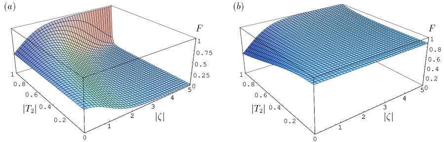
Figure 7: The fidelity of teleportation of a squeezed vacuum state ($\zeta_{0}$ $\!=$ $\!0.5$) is shown as a function of $|\zeta|$ and $|T_{2}|$ ($|T_{1}|$ $\!=$ $\!1$, $\tilde{\varphi}$ $\!=$ $\!0$) for the displacement $(a)$ $\Delta(\gamma^{\prime})$ $\!=$ $\!\gamma^{\prime}$ and $(b)$ $\Delta(\gamma^{\prime})$ $\!=$ $\!|T_{2}/T_{1}|\gamma^{\prime}$ [Eqs. (42) and (43)].

In the two figures, the fidelity for teleporting a squeezed vacuum state is shown as a function of the squeezing parameter $|\zeta|$ of the TMSV and the transmission coefficient $|T_{2}|$ for the case when the source of the TMSV is in Alice’s hand, i.e., $|T_{1}|$ $\!=$ $\!1$. Figure 7$(a)$ shows the result that is obtained for $\Delta(\gamma^{\prime})$ $\!=$ $\!\gamma^{\prime}$. It is seen that when $|T_{2}|$ is not close to unity, then the fidelity reduces, with increasing $|\zeta|$, below the classical level (realized for $|\zeta|$ $\!=$ $\!0$). In contrast, the displacement $\Delta(\gamma^{\prime})$ $\!=$ $\!e^{i\tilde{\varphi}}\lambda\gamma^{\prime}$ with $\lambda$ from Eq. (43) ensures that the fidelity exceeds the classical level [Fig. 7$(b)$].

At this point the question may arise of whether the choice of $\lambda$ according to Eq. (43) is the best one or not. For example, from inspection of Eq. (40) it could possibly be expected that $\lambda$ $\!=$ $\!C_{2}/|S|$ be also a a good choice. To answer the question, we note that in the formulas for the teleported quantum state and the fidelity $\lambda$ can be regarded as being an arbitrary (positive) parameter that must not necessarily be given by Eq. (43). Hence for chosen signal state and given value of $|\zeta|$, the value of $\lambda$ (and thus the value of the displacement) that maximizes the teleportation fidelity can be determined. Examples of the fidelity (as a function of $|\zeta|)$ that can be realized in this way are shown in

Figure 8: The fidelity of teleportation of $(a)$ a squeezed vacuum state ($\zeta_{0}$ $\!=$ $\!0.88$, i.e., $\bar{n}$ $\!\approx$ $\!1$) and $(b)$ a single-photon Fock state ($N$ $\!=$ $\!1$) is shown as a function of $|\zeta|$ ($|T_{1}|$ $\!=$ $\!1$, $|T_{2}|$ $\!=$ $\!0.9$, $\tilde{\varphi}$ $\!=$ $\!0$). The parameter $\lambda$ in the displacement $\Delta(\gamma^{\prime})$ $\!=$ $\!\lambda\gamma^{\prime}$ is chosen such that maximum fidelity is realized. For comparison, the fidelities that are realized for $\lambda$ $\!=$ $\!|T_{2}/T_{1}|$ (dashed line) and $\lambda$ $\!=$ $\!C_{2}/|S|$ (dotted line) are shown.

Fig. 8 for teleporting squeezed and number states according to Eqs. (2) and (65), respecticvely. The figure reveals that for not too small values of $|\zeta|$, that is, in the proper teleportation regime, the state-independent choice of $\lambda$ according to Eq. (43) is indeed the best one.

Figure 9 illustrates the dependence of the teleportation fidelity on the squeezing parameter $|\zeta|$ of the TMSV and the transmission coefficient $|T_{2}|$ ($|T_{1}|$ $\!=$ $\!1$) for squeezed and number states. It is seen that with increasing value of $|\zeta|$ the fidelity is rapidly saturated below unity, because of absorption. Even if the TMSV were infinitely entangled, the fidelity would be noticeably smaller than unity in practice.

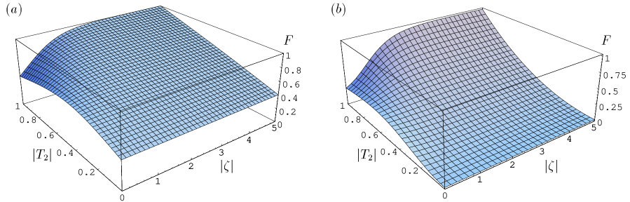
Figure 9: The fidelity of teleportation of $(a)$ a squeezed coherent state ($\zeta_{0}$ $\!=$ $\!0.5$, $\alpha_{0}$ $\!\approx$ $\!0.7$, i.e., $\bar{n}$ $\!\approx$ $\!1$) and $(b)$ a single-photon Fock state ($N$ $\!=$ $\!1$) is shown as a function of $|\zeta|$ and $|T_{2}|$ ($|T_{1}|$ $\!=$ $\!1$, $\tilde{\varphi}$ $\!=$ $\!0$, $\lambda$ $\!=$ $\!|T_{2}/T_{1}|$).

Only when $|T_{2}|$ is very close to unity, the fidelity substantially exceeds the classical level and becomes close to unity. Note that the classical level is much smaller for number states than for squeezed states. Hence, it is principally impossible to realize quantum teleportation over distances that are comparable with those of classical channels. The result is not unexpected, because the scheme is based on a strongly squeezed TMSV, which corresponds to an entangled macroscopic (at least mesoscopic) quantum state. As shown in Section 2.2, such a state decays very rapidly, so that the potencies inherent in it cannot be used in praxis.

Figure 10: The fidelity of teleportation of $(a)$ squeezed vacuum states (curve $1$: $\zeta_{0}$ $\!=$ $\!0.88$, i.e., $\bar{n}$ $\!\approx$ $\!1$; curve $2$: $\zeta_{0}$ $\!=$ $\!1.54$, i.e., $\bar{n}$ $\!\approx$ $\!5$; curve $3$: $\zeta_{0}$ $\!=$ $\!1.87$, i.e., $\bar{n}$ $\!\approx$ $\!10$) and $(b)$ Fock states (curve $1$: $N$ $\!=$ $\!1$; curve $2$: $N$ $\!=$ $\!5$; curve $3$: $N$ $\!=$ $\!10$) is shown as a function of the transmission length $l_{2}$ ($|T_{1}|$ $\!=$ $\!1$, $\tilde{\varphi}$ $\!=$ $\!0$, $\lambda$ $\!=$ $\!|T_{2}/T_{1}|$).

In order to illustrate the ultimate limits in more detail, we have plotted in Fig. 10 the dependence of the teleportation fidelity on the transmission length $l_{2}$ ($l_{1}$ $\!=$ $\!0$) for squeezed and number states, assuming an infinitely squeezed TMSV. It is seen that with increasing transmission length the fidelity very rapidly decreases, and it approaches the classical level on a length scale that is much shorter than the absorption length. In particular, the distance over which a squeezed state can really be teleported drastically decreases with increasing squeezing. The same effect is observed for number states when the number of photons increases. In other words, for chosen distance, the amount of information that can be transferred quantum mechanically is limited, so that essential information about the quantum state that is desired to be teleported is lost. Obviously, this limitation reflects the effect of saturation of entanglement, as it is illustrated in Fig. 5.

Figure 11: The optimal distance $l_{1}$ from Alice to the position of an infinitely squeezed TMSV, for which maximum teleportation fidelity is realized, is shown as a function of the teleportation distance $l_{12}$ $\!=$ $\!l_{1}$ $\!+$ $\!l_{2}$ ($\tilde{\varphi}$ $\!=$ $\!0$, $\lambda$ $\!=$ $\!|T_{2}/T_{1}|$) for $(a)$ squeezed states (curve $1$: $\zeta_{0}$ $\!=$ $\!0.78$, $\alpha_{0}$ $\!=$ $\!0.5$, i.e., $\bar{n}$ $\!\approx$ $\!1$; curve $2$: $\zeta_{0}$ $\!=$ $\!1.44$, $\alpha_{0}$ $\!=$ $\!1$, i.e., $\bar{n}$ $\!\approx$ $\!5$; curve $3$: $\zeta_{0}$ $\!=$ $\!1.63$, $\alpha_{0}$ $\!=$ $\!2$, i.e., $\bar{n}$ $\!\approx$ $\!10$) and $(b)$ Fock states (curve $1$: $N$ $\!=$ $\!1$; curve $2$: $N$ $\!=$ $\!5$; curve $3$: $N$ $\!=$ $\!10$). The insets show the dependence of the fidelity on the position of the source of the TMSV for $l_{12}/l_{\rm A}$ $\!=$ $\!0.1$.

So far we have considered the extremely asymetrical equipment where the source of the TMSV is in Alice’ hand ($|T_{1}|$ $\!=$ $\!1$, i.e., $|l_{1}|$ $\!=$ $\!0$). Whereas for perfect teleportation the source of the TMSV can be placed anywhere, in praxis the teleportation fidelity sensitively depends on the position of the source of the TMSV. In Fig. 11, examples of the optimal distance $l_{1}$ from Alice to the source of an infinitely squeezed TMSV (i.e., the distance for which maximum fidelity is realized) is shown, again for squeezed and number states, as a function of the distance $l_{12}$ $\!=$ $\!l_{1}$ $\!+$ $\!l_{2}$ between Alice and Bob (i.e., the transmission length). It is seen that the optimal position of the source of the TMSV is state-dependent, and it is always nearer to Alice than to Bob ($0$ $\!\leq$ $\!l_{1}$ $\!<$ $\!0.5\,l_{12}$). With increasing value of $l_{12}$ the value of $l_{1}$ approaches $0.5\,l_{12}$, and one could thus think that a symmetrical equipment would be the best one. Unfortunately, this is not the case, because the transmission lengths are essentially too large for true quantum teleportation. What were (optimally) observed would be the classical level at best.

4 Summary and conclusions

When entangled light is transmitted through optical devices, losses always give rise to entanglement degradation. In particular, after propagation of the two modes of a TMSV through fibers the available entanglement can be drastically reduced. Unfortunately, quantifying entanglement of mixed states in infinite-dimensional Hilbert spaces has been close to impossible. Therefore, estimates and upper bounds for the entanglement content have been developed.

In order to quantify the entanglement degradation of a TMSV more precisely, we have considered the distance of the output Gaussian state to the set of separable Gaussian states measured by the relative entropy. It has the advantage that separable states obviously correspond to zero distance. Although one has yet no proof that there does not exist a non-Gaussian separable state which is closer to the Gaussian state under consideration than the closest separable Gaussian state, one has good reason to think that it is even an entanglement measure. In any case, it is a much better bound than the one obtained by convexity. In particular, it clearly demonstrates the drastic decrease of entanglement of the output state with increasing entanglement of the input state. Moreover, one observes saturation of entanglement transfer; that is, the amount of entanglement that can maximally be contained in the output state is solely determined by the transmission length and does not depend on the amount of entanglement contained in the input state.

In continuous-variable quantum teleportation it is commonly assumed that Alice and Bob share an infinitely squeezed TMSV. Since the TMSV state as an effectively macroscopic (at least mesoscopic) entangled quantum state which rapidly decays, proper quantum teleportation can be expected to be possible only over distances that are much more shorter than the (classical) absorption length. Our analysis shows that this is indeed the case. The strong entanglement degradation dramatically limits the amount of information that can be transferred quantum mechanically over longer distances.

Because of this limitation, quantum teleportation becomes state-dependent, that is, without additional knowledge of the state that is desired to be teleported over some finite distance it is principally impossible to decide whether the teleported state is sufficiently close to the original state. It is worth noting that both the coherent displacement that must be performed by Bob and the position of the source of the TMSV should not be chosen independently of the fiber lengths. In particular, an asymmetrical equipment, where the source of the TMSV is placed nearer to Alice than to Bob, is suited for realizing the largest possible teleportation fidelity and not a symmetrical one.

Throughout this paper we have restricted our attention to (quasi-)monochromatic fields. Using wave packets, the ultimate limits of quantum teleportation are not only determined by absorption but also by dispersion. Due to dispersion, the two wave packets unavoidably change their forms during propagation over longer distances, and the problem of mode mismatching in Alice’s homodyne measuerment and Bob’s coherent displacement appears. The corresponding quantum efficiencies diminish, and hence the width of the Gaussian with which the Wigner function of the original quantum state is convolved is effectively increased. As a result, the teleportation fidelity is reduced. It can be expected that the effect sensitively depends on the position of the source of the TMSV. In order to understand the details, a separate analysis is required, which will be given elsewhere.

References

- [1] S.L. Braunstein and H.J. Kimble, Phys. Rev. Lett. 80, 869 (1998).
- [2] V. Vedral and M.B. Plenio, Phys. Rev. A 57, 1619 (1998).
- [3] T. Hiroshima, Phys. Rev. A 63, 022305 (2001).
- [4] L. Knöll, S. Scheel, E. Schmidt, D.-G. Welsch, and A.V. Chizhov, Phys. Rev. A 60, 4716 (1999).
- [5] S. Scheel, T. Opatrný, and D.-G. Welsch, Paper presented at the International Conference on Quantum Optics 2000, Raubichi, Belarus, May 28-31, 2000, arXiv: quant-ph/0006026.
- [6] E.M. Rains, Phys. Rev. A 60, 179 (1999).
- [7] S. Wu and Y. Zhang, Phys. Rev. A 63, 012308 (2001).
- [8] S. Scheel, L. Knöll, T. Opatrný, and D.-G. Welsch, Phys. Rev. A 62, 043803 (2000).
- [9] R. Simon, Phys. Rev. Lett. 84, 2726 (2000).
- [10] L.-M. Duan, G. Giedke, J.I. Cirac, and P. Zoller, Phys. Rev. Lett. 84, 2722 (2000).
- [11] J. Lee, M.S. Kim, and H. Jeong, Phys. Rev. A 62, 032305 (2000).