Mesoscopic interference

Abstract

We analyze a double-slit experiment when the interfering particle is “mesoscopic” and one endeavors to obtain Welcher Weg information by shining light on it. We derive a compact expression for the visibility of the interference pattern: coherence depends on both the spatial and temporal features of the wave function during its travel to the screen. We set a bound on the temperature of the mesoscopic particle in order that its quantum mechanical coherence be maintained.

I Introduction

The double-slit experiment is one of the simplest and most fundamental examples in quantum mechanics. However, in spite of its simplicity, its explanation is subtle and brings to light some of the most intriguing features of the quantal description of nature. According to Feynman, Leighton and Sands [1] “[this is] a phenomenon which is impossible, absolutely impossible, to explain in any classical way, and which has in it the heart of quantum mechanics. In reality, it contains the only mystery.”

It is not exaggerated to say that our comprehension of nature has been shaped by our advances in interference and interferometry, both at an experimental and a theoretical level. Technological progress has played a primary role: experiments that were undreamed of until a few years ago can be carried out nowadays. Double-slit interference experiments with photons [2], neutrons [3], electrons [4], atoms [5] and small molecules [6, 7] can now be routinely performed. All these systems can be considered microscopic, essentially because they are “elementary,” can be described in terms of a wave function and their evolution is governed by the Schrödinger equation with amazing accuracy.

The aim of the present paper is to discuss the interference of mesoscopic systems. “Mesoscopic” objects are neither microscopic nor macroscopic. Although we shall not attempt to give a rigorous definition of “mesoscopicity” (we do not know any), we shall think of systems that can be described by a wave function, yet are made up of a significant number of elementary constituents, such as atoms. Most important, they are characterized by a nontrivial internal structure that can have both quantal and classical features. A significant example, on which we shall focus our attention, is a molecule of fullerene, made up of 60 nuclei of Carbon and 360 electrons, for a total of about $10^{3}$ “elementary” constituents. Although fullerenes are fully quantum mechanical systems, they also have macroscopic-like features and emit thermal (blackbody) radiation [8, 9, 10]. Very recently the quantum interference of fullerene molecules (C₆₀ and C₇₀) has been observed in a series of pioneering experiments performed in Vienna [11, 12]. Our aim is to analyze the interference of fullerene from a theoretical and fully quantum mechanical viewpoint.

The discussion that follows is of general validity. However, as S.J. Gould masterly suggests [13] “frontal attacks upon generalities inevitably lapse into tedium or tendentiousness. The beauty of nature lies in detail; the message, in generality. Optimal appreciation demands both, and I know no better tactic than the illustration of exciting principles by well-chosen particulars.” Although our analysis applies to any molecule or system endowed with an internal structure, the kind of questions that pop up in one’s mind when one ponders over the properties and complexity of C₆₀ make the following discussion very fascinating.

This paper contains tutorial sections as well as original material. We start by setting up the notation and outlining the physics of the double-slit experiment in Section 2. Although the content of this section is usually the subject of elementary textbooks of quantum mechanics, our analysis is original: we derive the double-slit diffraction pattern by solving the time-dependent Schrödinger equation, with given (and well chosen) initial conditions. In Section 3 we revisit Heisenberg’s microscope [14], analyzing an experimental configuration aimed at determining which slit the particle goes through. This example as well can be found in introductory chapters of textbooks of quantum mechanics; however, we introduce here a novel element of discussion, “postponing” the determination of the particle’s route in a way that will turn out to be interesting and significant for the subsequent analysis. The central part of the manuscript are Sections 4 and 5. Section 4 contains a model calculation leading to an (almost) exact formula for the visibility of the interference pattern when a complex molecule (“fullerene”) passes through a double slit and is illuminated by laser light of given wavelength. The visibility of the interference pattern depends on the laser wavelength (as expected), but also, interestingly, on the lifetime of the reemission process. We tried to keep the discussion at a reasonably elementary level, adding two appendices in which some relevant notions of advanced quantum mechanics and quantum electrodynamics are explained. Section 5 contains a discussion of what we will call “interference of mesoscopic systems.” A novel formula will be derived, relating the features of the interference pattern to the temperature of the fullerene molecule. A “decoherence temperature” will be defined as a function of some intrinsic properties of the molecule (such as its area and velocity) and the geometry of the experimental setup (such as the separation of the slits and the distance between slits and screen). Section 6 is devoted to our concluding remarks. Our analysis will motivate us to ask in which sense a molecule of fullerene can be considered “microscopic” and, by contrast, when it is more appropriate to think of it in mesoscopic terms. This will lead us to wonder about the significance of quantum (de)coherence.

II Double-slit interference

We start by looking at the simplest quantum mechanical experiment: consider a quantum system described by a wave packet $\Psi_{\rm in}$, impinging on a double slit. We assume that the wave packet travels along direction $+z$ and its transverse coherence length is larger than the distance between the slits, so that the two wave packets emerging from the slits are coherent with each other. This is a fundamental requirement in interferometry, both at a quantal and classical level (although the quantal situation has a different “charm” if one thinks that the experiment is performed by accumulating events pertaining to single quantum systems [15]). The slits are parallel to $y$, have width $a$ and are separated by a distance $d$, along direction $x$. The geometry of our arrangement is outlined in Figure 1.

We shall assume that the wave functions (the one impinging on the slit and those emerging from it) can be approximated by Gaussians. In general, a Gaussian wave packet has the form

$$\langle\mbox{\boldmath$x$}|\Psi\rangle=\Psi(\mbox{\boldmath$x$},t=0)=\psi_{x}(x)\psi_{y}(y)\psi_{z}(z)$$ (1)

where $|\Psi\rangle$ is the quantum state and

$$\psi_{x}(x)\!\! = \!\!\frac{1}{(2\pi\delta x^{2})^{1/4}}$$ (3)

$$\times\exp\left(-\frac{1-i\eta_{x}}{4\delta x^{2}}(x-\bar{x})^{2}+\frac{i}{\hbar}\bar{p}_{x}x-i\phi_{x}\right)$$

(analogously for $y$ and $z$), where $\eta_{x}$ and $\phi_{x}$ are real constants, $\bar{x}$ and $\bar{p}_{x}$ are the average position and momentum, respectively, and their standard deviations $\delta x$ and $\delta p_{x}$ satisfy the relation

$$\delta x\delta p_{x}=(1+\eta_{x}^{2})^{\frac{1}{2}}\frac{\hbar}{2}\geq\frac{\hbar}{2},$$ (5)

so that (LABEL:eq:gaussgenxyz) has the minimum uncertainty for $\eta_{x}=0$. The evolution of the packet (1) in free space $\langle\mbox{\boldmath$x$}|e^{-ip^{2}t/2m\hbar}|\Psi\rangle$ is readily evaluated and maintains a Gaussian form. One gets

$$\psi_{x}(x,t) = \frac{1}{(2\pi\delta x^{2}(t))^{1/4}}$$ (8)

$$\times\exp\left(-\frac{1-i\eta_{x}(t)}{4\delta x^{2}(t)}(x-\bar{x}(t))^{2}\right.$$

$$\left.+\ \frac{i}{\hbar}\bar{p}_{x}x-i\phi_{x}(t)\right),$$

where

$$\bar{x}(t) = \bar{x}(0)+\frac{\bar{p}_{x}}{m}t,$$ (9)

$$\eta_{x}(t) = \eta_{x}(0)+2\frac{\delta p_{x}^{2}}{m\hbar}t,$$ (10)

$$\delta x^{2}(t) = \frac{\hbar^{2}}{4\delta p_{x}^{2}}(1+\eta_{x}^{2}(t)),$$ (11)

$$\phi_{x}(t) = \phi_{x}(0)+\frac{\bar{p}_{x}^{2}}{2m\hbar}t$$ (13)

$$+\ \frac{1}{2}\left(\arctan\eta_{x}(t)-\arctan\eta_{x}(0)\right).$$

Obviously, the spread $\delta p_{x}$ and average momentum $\bar{p}_{x}$ remain unchanged during the free evolution.

FIG. 1.: A quantum object impinging on a double slit. The velocity of the wave packet is in direction $+z$, the slits have width $a$ and are separated by a distance $d$.

The preceding formulas are of general validity. Our initial state is that emerging from the two slits

$$|\Psi_{0}\rangle=\frac{1}{\sqrt{N}}(|\Psi_{\ell}\rangle+|\Psi_{r}\rangle),$$ (14)

where $\ell$ and $r$ stand for “left” and “right” respectively, $N$ is a normalization factor (see later) and

$$\Psi_{\ell,r}(\mbox{\boldmath$x$})=\langle\mbox{\boldmath$x$}|\Psi_{\ell,r}\rangle=\psi_{\ell,r}(x)\psi_{y}(y)\psi_{z}(z).$$ (15)

All wave functions have the Gaussian form (LABEL:eq:gaussgenxyz) with

$$\bar{x}_{\ell,r}(0) = \mp\frac{d}{2},$$ (16)

$$\bar{y}(0) = \bar{z}(0)=0,$$ (17)

$$\bar{p}_{z} = \hbar k_{0},$$ (18)

$$\bar{p}_{x} = \bar{p}_{y}=0,$$ (19)

$$N = \parallel|\Psi_{\ell}\rangle+|\Psi_{r}\rangle\parallel^{2}$$ (20)

$$= 2\left(1+\exp\left(-\frac{d^{2}\delta p_{x}^{2}}{2\hbar^{2}}\right)\right),$$ (21)

so that the initial average positions of the two wave packets are $(\mp d/2,0,0)$ and their average momentum $\hbar k_{0}$ is in direction $+z$. We see that $N\simeq 2$ if the left and right packets are well separated ($d\gg\hbar/\delta p_{x}$). As already stressed, we are assuming that the wave function after the slits can be written as a “double Gaussian.” This is, for example, the approach of Feynman and Hibbs [16]. The evolution yields

$$|\Psi(t)\rangle=e^{-ip^{2}t/2m\hbar}|\Psi_{0}\rangle$$ (22)

and interference is observed at a screen perpendicular to $z$, placed at a distance $z=L$ from the plane of the slits. The problem becomes essentially one dimensional (the relevant coordinate being $x$) and the position probability distribution at the screen reads

$$\!\!\!\!\!\!|\Psi(\mbox{\boldmath$x$},t_{0})|^{2}$$ (23)

$$=|\langle\mbox{\boldmath$x$}|\Psi(t_{0})\rangle|^{2}$$ (24)

$$\equiv\frac{1}{N}|\Psi_{\ell}(\mbox{\boldmath$x$},t_{0})+\Psi_{r}(\mbox{\boldmath$x$},t_{0})|^{2}$$ (25)

$$=\frac{1}{N\sqrt{2\pi\delta x^{2}(t_{0})}}\left[\exp\left(-\frac{\left(x+\frac{d}{2}\right)^{2}}{2\delta x^{2}(t_{0})}\right)\right.$$ (26)

$$\left.\quad+\ \exp\left(-\frac{\left(x-\frac{d}{2}\right)^{2}}{2\delta x^{2}(t_{0})}\right)\right.$$ (27)

$$\left.\quad+\ 2\exp\left(-\frac{x^{2}+\left(\frac{d}{2}\right)^{2}}{2\delta x^{2}(t_{0})}\right)\cos\left(\frac{\eta_{x}(t_{0})d}{2\delta x^{2}(t_{0})}\;x\right)\right]$$ (28)

$$\quad\times\;|\psi_{y}(y,t_{0})|^{2}|\psi_{z}(z,t_{0})|^{2},$$ (29)

(30)

where $t_{0}=mL/\hbar k_{0}$ is the time of arrival of the wave packet at the screen.

This analysis is of general validity. However, in order to concentrate our attention on a concrete physical problem, we shall focus on the experiment [11] and take the slits to have width $a$ and to be separated by a distance $d=2a$. The intensity at the screen is

$$I(x) = \langle\Psi(t_{0})|x\rangle\langle x|\Psi(t_{0})\rangle$$ (31)

$$= \int dydz|\Psi(x,y,z,t_{0})|^{2},$$ (32)

which, due to normalization, is equal to (30) without the factor $|\psi_{y}(y,t)|^{2}|\psi_{z}(z,t)|^{2}$. We set $a=50$nm, $d=100$nm, $L=1.22$m, $m=1.197\cdot 10^{-24}$kg and consider a beam with $\bar{v}_{z}=128$m/s, so that one gets $k_{0}=\bar{v}_{z}m/\hbar=1.46\cdot 10^{12}$m^-1, $\lambda_{0}=4.3$pm and $t_{0}=9.47$ms. These values are taken from the latest Vienna experiment [12]. One of the advantages of focusing on a concrete physical example is that one gets a feeling for the numbers. This is particularly important when one deals with systems that can be properly considered mesoscopic (fullerene has a mass $m\simeq 720$u and is made up of $\simeq 10^{3}$ particles). One of the main ideas to be discussed in this paper is that coherence (i.e. the possibility of observing an interference pattern) is a quantitative issue: if the experimenter is able to keep under control all disturbances/noises/interactions in the setup, even a mesoscopic (or, in principle, macroscopic) system will preserve its coherence and display a double-slit interference pattern. We shall come back to this point in the next sections.

In the case considered above, we can choose $\delta x(0)\simeq a$. The results one obtains are completely independent of this choice if one looks at the far-field interference pattern, namely $\delta x(t_{0})\gg\delta x(0)$, i.e. $\eta_{x}(t_{0})\gg\eta_{x}(0)$. This is our case and we get from Eqs. (11) (far field)

$$\eta_{x}(t_{0}) \simeq 2\frac{\delta p_{x}^{2}}{m\hbar}t_{0},$$ (33)

$$\delta x(t_{0}) \simeq \frac{\hbar}{2}\frac{\eta_{x}(t_{0})}{\delta p_{x}}\simeq\frac{\delta p_{x}}{m}t_{0}$$ (34)

and

$$\frac{\eta_{x}(t_{0})d}{2\delta x^{2}(t_{0})}\simeq\frac{dm}{\hbar t_{0}}=\frac{2\pi}{X},$$ (35)

$$\quad\mbox{with}\quad X=\frac{ht_{0}}{md}=\frac{2\pi L}{k_{0}d}=52.46\mu{\rm m}.$$ (36)

Hence we can rewrite the intensity pattern

$$I(x)\simeq\frac{e^{-x^{2}/2\delta x^{2}(t_{0})}}{\sqrt{2\pi\delta x^{2}(t_{0})}}\left[1+\cos\left(2\pi\frac{x}{X}\right)\right],$$ (37)

where we neglected $a=d/2$ with respect to $\delta x(t_{0})$ in the Gaussian envelope functions in (30). The intensity at the screen is shown in Figure 2. Notice that the interference pattern has been obtained by simply solving the Schrödinger equation (free evolution in vacuum), as it should. The only free parameter is $\delta p_{x}$, which is determined by imposing the dispersion at the screen $\delta x(t_{0})=33.7\mu$m, which implies, by (34), $\delta p_{x}=4.26\cdot 10^{-27}$kg m/s.

FIG. 2.: The interference pattern (37).

It is interesting to observe that the minimum spatial width at the slits $\delta x(0)$ that can be chosen is constrained by the uncertainty relations (5) with $\eta_{x}(0)=0$ and reads $\delta x(0)=12.4\mbox{nm}\simeq a/4$, so that the position probability density at the slit boundary is reduced to 10% of its maximum value. This suggests that the choice of Gaussian wave packets at the slits is not optimal; a better wave function could be a bell-shaped function flattened at the top. Notice also that, as already stressed, the parameter $\delta_{x}(0)$ does not enter in the expression of the intensity pattern (37) and only guarantees the internal consistence of the calculation. In the same spirit of other calculations aimed at analyzing wave-packet effects [16, 17, 18], our analysis complements those based on the plane-wave approximation [19, 20].

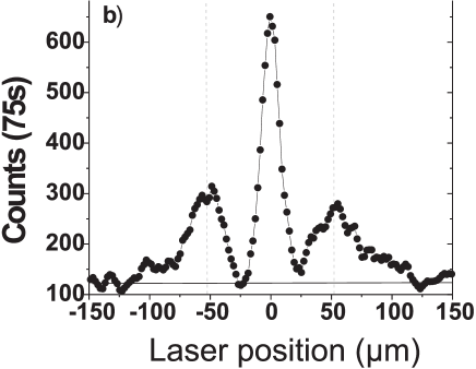
FIG. 3.: Interference of C₆₀: experimental results [12]. (Courtesy of the Vienna group.) Compare with Figure 2, where the (only) free parameter $\delta x(t_{0})$ has been adjusted in order to reproduce the experimental data. (“Laser position” in this figure is simply the screen coordinate.)

The beautiful experimental results obtained by the Vienna group are shown in Figure 3. Notice the high visibility, obtained with a well collimated molecular beam and a careful technique of velocity selection [12]. The asymmetry of the data may be ascribed to the velocity selection technique. By comparing Figure 3 with Figure 2, obtained in the hypothesis of a double-Gaussian initial state, by setting the (only) free parameter $\delta x(t_{0})=33.7\mu$m, one is led to think that only a few (say 2 or 3) slits of the diffraction grating are coherently illuminated by each fullerene molecule in the beam. The detailed features of a double-slit experiment for large molecules are still under investigation and there are interesting proposals concerning a reduced “effective” slit width [21, 11]. In our “minimal” calculation these additional effects have not been considered.

III The Heisenberg-Bohm microscope revisited

Interference disappears if one endeavors to obtain Welcher Weg information. Let us follow Bohm’s discussion [18] of a double-slit version of Heisenberg’s microscope [14]. The experiment is sketched in Figure 4(a). The situation is analogous to that described in the preceding section, but now a laser beam parallel to the slits ($y$ direction) is shined at the exit of the slits. The laser light has wavelength $\lambda_{\rm L}$ and the laser spot is larger than $d$, the distance between the slits. If a photon is scattered off the interfering particle, the momentum of the latter becomes uncertain of the quantity

$$\triangle p\simeq h/\lambda_{\rm L},$$ (38)

which “shakes” the interference pattern at the screen by the quantity

$$\triangle\theta\simeq\frac{\triangle p}{p}\simeq\frac{h}{\lambda_{\rm L}p}\quad\Leftrightarrow\quad\triangle x\simeq\frac{h}{\lambda_{\rm L}p}L,$$ (39)

where $\theta\simeq x/L$. On the other hand, from Eq. (37),

$$I(x)\propto 1+\cos\left(2\pi\frac{x}{X}\right)=1+\cos\left(\frac{pd\theta}{\hbar}\right),$$ (40)

so that the distance between a minimum and the adjacent maximum at the screen is

$$\triangle\theta_{M}=\frac{h}{2pd}\quad\Leftrightarrow\quad\triangle x_{M}\simeq\frac{h}{2pd}L$$ (41)

and the condition to observe interference reads

$$\triangle x\lesssim\triangle x_{M}\quad\Leftrightarrow\quad\lambda_{L}\gtrsim 2d.$$ (42)

In words, interference is preserved if the laser wavelength is larger than twice the distance between the slits because in such a case, by observing the scattered photon, one is unable to decide which slit the photon came from.

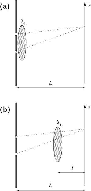
FIG. 4.: The Heisenberg-Bohm Welcher Weg experiment. (a) Standard setup. (b) Modified version: the laser light is shined at a distance $L-\ell$ from the slits.

Let us now consider a slightly different experiment [Figure 4(b)]. The laser spot is now focused at a distance $\ell<L$ from the screen. From simple geometrical considerations one gets

$$\triangle\theta\simeq\frac{\triangle p}{p}\simeq\frac{h}{\lambda_{\rm L}p}\quad\Leftrightarrow\quad\triangle^{\prime}x\simeq\frac{h}{\lambda_{\rm L}p}\ell$$ (43)

and the condition to observe interference reads now

$$\triangle^{\prime}x\lesssim\triangle x_{M}\quad\Leftrightarrow\quad\lambda_{L}\gtrsim 2d\frac{\ell}{L}.$$ (44)

The physical reason is simple: if the laser spot is far from the slits, the interfering waves converging to a given point of the screen are closer to each other and one needs light of smaller wavelength to resolve them. Notice that when $\ell\ll L$ the laser wavelength needed to destroy the interference pattern becomes very small!

The situation just described is somewhat reminiscent of Wheeler’s “delayed choice” [22], the important difference being that in our case the longer the choice (to determine the route) is postponed, the more “effective” the measurement needs to be.

IV Determining the trajectory by a laser beam

So far the interfering system has been a structureless particle. In the previous section we endeavored to obtain information on the particle’s route by scattering light on the system (notice also that the scattering process was assumed to occur instantaneously). However, we aim at describing a more complicated physical picture, that can arise when the interfering system is endowed with a richer internal physical structure. For instance, consider the interference of C₆₀ molecules: in order to obtain path information, one might shine laser light on the molecule after it has gone through the slits, exactly like with the Heisenberg-Bohm microscope. However, the situation would be different, because the molecule can be regarded as a mesoscopic system, whose inner structure is rich enough to give rise to more complicated processes, involving lifetimes, emission of blackbody radiation [9, 10] and complex ionization processes [8, 23, 24, 25]. Unlike with the “elementary” particle in the Heisenberg-Bohm microscope, a fullerene molecule can absorb one or more photons and undergo internal structural rearrangements.

It is therefore of great interest to try and understand how the coherence properties of a “mesoscopic” system are modified when light of a given wavelength is shined on it, but the reemission process takes place after a certain characteristic time. This brings us conceptually closer to the situation envisaged in Figure 4(b). Needless to say, this is a simplified picture of what would occur in the experiment performed by the Vienna group [11] if one would try to obtain information about the path of a fullerene molecule by illuminating it with an intense laser beam. We shall come back to this point in the next section, where a more realistic model will be considered. For the moment, according to what we saw in the preceding section, the minimal requirement to maintain quantum coherence and preserve the interference pattern is the condition (44). However, we shall see that this is not the only criterion.

We start our considerations from a simple field-theoretical model. This model is too elementary to reflect the complicated physical effects that take place, for instance, in a fullerene molecule. However, it has two main advantages: first, by virtue of its simplicity, it admits an almost exact solution; second, in spite of its simplicity, it captures some fundamental aspects related to the notion of quantum mechanical coherence, when the interfering system is more complicated than, say, an electron or a neutron. Consider the Hamiltonian [26]

$$H = H_{0}+V+V_{\rm L},$$ (45)

$$H_{0} = \frac{\mbox{\boldmath$p$}^{2}}{2m}+\hbar\omega_{0}|e\rangle\langle e|+\sum_{i}\hbar\omega_{i}a^{\dagger}_{i}a_{i},$$ (46)

$$V = \sum_{i}\left(\Phi_{i}e^{i\mbox{\boldmath$k$}_{i}\cdot\mbox{\boldmath$x$}}|e\rangle\langle g|a_{i}+\mbox{h.c.}\right),$$ (47)

$$V_{\rm L}(t) = \left(\Phi_{\rm L}(t)e^{-i\omega_{\rm L}t+i\mbox{\boldmath$k$}_{\rm L}\cdot\mbox{\boldmath$x$}}|e\rangle\langle g|+\mbox{h.c.}\right),$$ (48)

where

$$\Phi_{i} = -ie\mbox{\boldmath$d$}\cdot\mbox{\boldmath$\epsilon$}_{i}\sqrt{\frac{\hbar\omega_{i}}{2\epsilon_{0}L^{3}}},$$ (49)

$$\Phi_{\rm L}(t) = -ie\mbox{\boldmath$d$}\cdot\mbox{\boldmath$E$}_{\rm L}(t),$$ (50)

$$d = \langle e|\mbox{\boldmath$x$}|g\rangle.$$ (51)

We work in 3 dimensions. The above Hamiltonian describes a two-level system (to be called “molecule”) of mass $m$, (center of mass) position $x$ and momentum $p$, coupled to the electromagnetic field, whose operators obey boson commutation relations

$$[a_{i},a^{\dagger}_{j}]=\delta_{ij},$$ (52)

where the indexes $i,j$ are shorthand notations for the photon momentum $\mbox{\boldmath$k$}_{i}$ and polarization $\lambda=1,2$. The ground state $|g\rangle$ has energy 0, while the excited state $|e\rangle$ has energy $\hbar\omega_{0}$. The molecule interacts with a (classical) laser, in the rotating-wave and dipole approximations. The laser has electric field $\mbox{\boldmath$E$}_{\rm L}$ and frequency $\omega_{\rm L}=c|\mbox{\boldmath$k$}_{\rm L}|$; we shall also assume that the laser beam is parallel to the $y$-axis. The quantities $-e\mbox{\boldmath$d$},\mbox{\boldmath$\epsilon$}_{i},\epsilon_{0},L^{3}$ in (50) are the electric dipole moment, photon polarization, vacuum permittivity and volume of the quantization box, respectively.

The state of the total system will be written

$$|\Psi_{\rm tot}\rangle=|\Psi,\alpha,n_{i}\rangle\equiv|\Psi\rangle\otimes|\alpha\rangle\otimes|n_{i}\rangle,$$ (53)

where $\Psi$ denotes the spatial part of the wave function of the molecule (in notation identical to that of Section 2), $\alpha=e,g$ and $n_{i}$ is the number of photons emitted in the $i$-mode during the $e$-$g$ transition. The state emerging from the two slits is

$$|\Psi_{0},g,0\rangle\equiv|\Psi_{0}\rangle\otimes|g\rangle\otimes|0\rangle,$$ (54)

where $|\Psi_{0}\rangle$ is given in (14). We assume that the laser beam is placed immediately beyond the slits and illuminates coherently both wave packets $|\Psi_{\ell}\rangle$ and $|\Psi_{r}\rangle$ in (14), like in Figure 4(a). After a laser pulse of duration $T$ such that $\int_{0}^{T}dt\;\Phi_{\rm L}(t)e^{-i\omega_{\rm L}t}/\hbar=\pi/2$, the molecule has absorbed a photon with probability 1 and the state reads

$$|\Psi_{\rm tot}\rangle=|e^{i\mbox{\boldmath$k$}_{\rm L}\cdot\mbox{\boldmath$x$}}\Psi_{0},e,0\rangle.$$ (55)

This is our “initial” state. Since $\mbox{\boldmath$k$}_{\rm L}$ is parallel to the $y$-axis, the molecule recoils along the vertical direction without modifying the properties of the interference pattern (in the $x$ direction). The spontaneous emission process is studied in Appendix A, where the evolution is readily computed in the Weisskopf-Wigner approximation [27, 28, 29] and yields

$$|\Psi_{\rm tot}(t)\rangle = e^{-i\omega_{0}t}e^{-\gamma t/2}|e^{-ip^{2}t/2m\hbar}e^{i\mbox{\boldmath$k$}_{\rm L}\cdot\mbox{\boldmath$x$}}\Psi_{0},e,0\rangle$$ (58)

$$+\sum_{i}e^{-i\omega_{i}t}\beta_{i}(t)$$

$$\times|e^{-ip^{2}t/2m\hbar}e^{i(\mbox{\boldmath$k$}_{\rm L}-\mbox{\boldmath$k$}_{i})\cdot\mbox{\boldmath$x$}}\Psi_{0},g,1_{i}\rangle,$$

where ($\alpha=e^{2}/4\pi\epsilon_{0}\hbar c$)

$$\gamma = \frac{2\pi}{\hbar^{2}}\sum_{i}|\Phi_{i}|^{2}\delta(\omega_{i}-\omega_{0})$$ (59)

$$= \frac{2\pi}{\hbar^{2}}\sum_{\lambda}\int d^{3}k\;\frac{e^{2}\hbar\omega}{2\epsilon_{0}(2\pi)^{3}}|\mbox{\boldmath$d$}\cdot\mbox{\boldmath$\epsilon$}_{\mbox{\boldmath$k$}\lambda}|^{2}\delta(\omega-\omega_{0})$$ (60)

$$= \frac{4}{3}\frac{\alpha\omega_{0}^{3}|\mbox{\boldmath$d$}|^{2}}{c^{2}},$$ (61)

is the decay rate (the third expression is the continuum limit), as given by the Fermi “golden” rule [30], and

$$\beta_{i}(t)=\frac{\Phi^{*}_{i}}{\hbar}\frac{1-e^{i(\omega_{i}-\omega_{0})t-\gamma t/2}}{(\omega_{i}-\omega_{0})+i\gamma/2}.$$ (62)

The spontaneous emission process of a photon is shown in Figure 5. The total momentum is conserved and the molecule recoils.

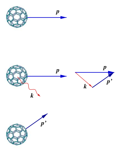
FIG. 5.: Spontaneous emission process of a photon.

We see that in (58) the internal degrees of freedom of the molecule get entangled with the photon field, so that the states in (58) are all orthogonal each other. We can now analyze the influence of the spontaneous emission process on the interference pattern, i.e. on the quantum mechanical coherence of the molecule. The intensity at the screen is readily written as

$$I^{\prime}(x) = \langle\Psi_{\rm tot}(t_{0})|x\rangle\langle x|\Psi_{\rm tot}(t_{0})\rangle$$ (63)

$$= \exp(-\gamma t_{0})\langle\Psi^{\mbox{\boldmath$k$}_{\rm L}}(t_{0})|x\rangle\langle x|\Psi^{\mbox{\boldmath$k$}_{\rm L}}(t_{0})\rangle$$ (66)

$$+\ \sum_{i}|\beta_{i}(t_{0})|^{2}$$

$$\quad\quad\times\langle\Psi^{\mbox{\boldmath$k$}_{\rm L}-\mbox{\boldmath$k$}_{i}}(t_{0})|x\rangle\langle x|\Psi^{\mbox{\boldmath$k$}_{\rm L}-\mbox{\boldmath$k$}_{i}}(t_{0})\rangle$$

$$= \exp(-\gamma t_{0})I_{\mbox{\boldmath$k$}_{\rm L}}(x)+\sum_{i}|\beta_{i}(t_{0})|^{2}I_{\mbox{\boldmath$k$}_{\rm L}-\mbox{\boldmath$k$}_{i}}(x),$$ (67)

(68)

where

$$|\Psi^{\mbox{\boldmath$k$}}(t_{0})\rangle=\exp\left(-i\frac{p^{2}}{2m\hbar}t_{0}\right)\exp(i\mbox{\boldmath$k$}\cdot\mbox{\boldmath$x$})|\Psi_{0}\rangle$$ (69)

is the free evolution of the “double Gaussian” wave packet that has (jointly) recoiled (due to photon emission and/or absorption) by momentum $\hbar\mbox{\boldmath$k$}$. In the position representation

$$\Psi^{\mbox{\boldmath$k$}}(\mbox{\boldmath$x$},t_{0}) = \langle\mbox{\boldmath$x$}|\exp\left(-i\frac{p^{2}}{2m\hbar}t_{0}\right)\exp(i\mbox{\boldmath$k$}\cdot\mbox{\boldmath$x$})|\Psi_{0}\rangle$$ (70)

$$= \frac{e^{-ip^{2}t_{0}/2m\hbar}e^{i\mbox{\boldmath$k$}\cdot\mbox{\boldmath$x$}}}{\sqrt{N}}[\Psi_{\ell}(\mbox{\boldmath$x$})+\Psi_{r}(\mbox{\boldmath$x$})].$$ (71)

The quantity $I_{\mbox{\boldmath$k$}_{\rm L}-{\mbox{\boldmath$k$}_{i}}}(x)$ represents the partial interference pattern of those molecules that have emitted a photon of momentum $\hbar\mbox{\boldmath$k$}_{i}$ (and absorbed a laser photon of momentum $\hbar\mbox{\boldmath$k$}_{\rm L}$). By applying the same method utilized for (30)-(32), it is straightforward to obtain

$$I_{\mbox{\boldmath$k$}}(x) = \int dydz|\Psi^{\mbox{\boldmath$k$}}(\mbox{\boldmath$x$},t_{0})|^{2}$$ (72)

$$= \frac{1}{N\sqrt{2\pi\delta x^{2}(t_{0})}}\left[\exp\left(-\frac{\left(x-v_{x}t_{0}+\frac{d}{2}\right)^{2}}{2\delta x^{2}(t_{0})}\right)\right.$$ (76)

$$\left.+\ \exp\left(-\frac{\left(x-v_{x}t_{0}-\frac{d}{2}\right)^{2}}{2\delta x^{2}(t_{0})}\right)\right.$$

$$\left.+\ 2\exp\left(-\frac{(x-v_{x}t_{0})^{2}+\left(\frac{d}{2}\right)^{2}}{2\delta x^{2}(t_{0})}\right)\right.$$

$$\left.\times\cos\left(\frac{\eta_{x}(t_{0})d}{2\delta x^{2}(t_{0})}(x-v_{x}t_{0})\right)\right]$$

$$= I\left(x-v_{x}t_{0}\right),$$ (77)

where $v_{x}=\hbar k_{x}/m$ is the $x$-component of the average velocity (remember that $\mbox{\boldmath$k$}_{0}$ is parallel to $z$, so that $v_{x}$ only gets a contribution from the emitted photon’s $k$). Neglecting $a=d/2$ with respect to $\delta x(t_{0})$ in the envelope function we obtain

$$I_{\mbox{\boldmath$k$}}(x) \simeq \frac{e^{-(x-v_{x}t_{0})^{2}/2\delta x^{2}(t_{0})}}{\sqrt{2\pi\delta x^{2}(t_{0})}}$$ (79)

$$\times\left[1+\cos\left(\frac{2\pi}{X}(x-v_{x}t_{0})\right)\right],$$

where we set $X=ht_{0}/md$, like in (35). By recalling that the laser beam is parallel to the $y$ direction, that is $k_{{\rm L}x}=0$, and by noting that $I_{\mbox{\boldmath$k$}}(x)$ in (77)-(79) depends only on $k_{x}$, the intensity pattern (68) reads

$$I^{\prime}(x)=\exp(-\gamma t_{0})I(x)+\sum_{i}|\beta_{i}(t_{0})|^{2}I_{-\mbox{\boldmath$k$}_{i}}(x).$$ (80)

As we can see, the interference pattern is made up of two terms: the first one is associated with those molecules that have not emitted any photon, the second one with those molecules that have emitted a photon and recoiled accordingly. Obviously, the latter term depends on the features of such emission.

Assume now that the spontaneous emission process is completely isotropic, i.e. the directions of the dipole moments $d$ in (50) of the molecules in the beam are completely random. In this case the last term in Eq. (80) is readily evaluated (see Appendix B) and yields

$$\left\langle\sum_{i}|\beta_{i}(t_{0})|^{2}I_{-\mbox{\boldmath$k$}_{i}}(x)\right\rangle$$ (81)

$$=(1-e^{-\gamma t_{0}})\int\frac{d\Omega_{\mbox{\boldmath$\bar{k}$}}}{4\pi}\;I_{-\mbox{\boldmath$\bar{k}$}}(x),$$ (82)

where $|\mbox{\boldmath$\bar{k}$}|=\omega_{0}/c$ and $\langle\dots\rangle$ denotes the average over the molecular dipole direction. By using (79), the last integral (average over the direction of the emitted photon) yields

$$\int d\Omega_{\mbox{\boldmath$\bar{k}$}}\;I_{-\mbox{\boldmath$\bar{k}$}}(x)$$ (83)

$$=2\pi\int_{-1}^{1}d\xi\;\frac{e^{-(x+\bar{v}t_{0}\xi)^{2}/2\delta x^{2}(t_{0})}}{\sqrt{2\pi\delta x^{2}(t_{0})}}$$ (84)

$$\quad\times\left[1+\cos\left(\frac{2\pi}{X}(x+\bar{v}t_{0}\xi)\right)\right],$$ (85)

where we set $\bar{v}_{x}/\bar{v}=\xi$. It is evident from this expression that when $\bar{v}t_{0}=X/2$ the cosine is averaged over the whole interval $2\pi$ and the second interference term in (80) is completely washed out. For smaller values of $\bar{v}t_{0}$ there is still some interference.

Let us focus on a realistic situation. Unlike in Section 2, we set here $X/\delta x(t_{0})=0.4$ for clarity of presentation, in order to get quite a few oscillations in the interference pattern (this will also enable us to obtain compact expressions). In this case $\bar{v}t_{0}<X/2\ll 2\delta x(t_{0})$ and the Gaussian envelope in (85) is practically constant over the range of integration. ($\exp(-X^{2}/8\delta x^{2}(t_{0}))=0.98$). We can then write

$$\int d\Omega_{\mbox{\boldmath$\bar{k}$}}\;I_{-\mbox{\boldmath$\bar{k}$}}(x)\simeq 2\pi\frac{e^{-x^{2}/2\delta x^{2}(t_{0})}}{\sqrt{2\pi\delta x^{2}(t_{0})}}$$ (86)

$$\quad\times\int_{-1}^{1}d\xi\;\left[1+\cos\left(\frac{2\pi}{X}(x+\bar{v}t_{0}\xi)\right)\right]$$ (87)

$$=4\pi\frac{e^{-x^{2}/2\delta x^{2}(t_{0})}}{\sqrt{2\pi\delta x^{2}(t_{0})}}$$ (88)

$$\quad\times\left[1+{\rm sinc}\left(\frac{\omega_{0}d}{c}\right)\cos\left(\frac{2\pi}{X}x\right)\right],$$ (89)

where ${\rm sinc}(x)\equiv\sin x/x$ and we used the equality $2\pi\bar{v}t_{0}/X=\omega_{0}d/c$. By plugging (89) and (82) into (80) we finally obtain

$$I^{\prime}(x)=\frac{e^{-x^{2}/2\delta x^{2}(t_{0})}}{\sqrt{2\pi\delta x^{2}(t_{0})}}\left[1+{\cal V}\left(\gamma t_{0},\frac{d}{\lambda_{0}}\right)\cos\left(\frac{2\pi}{X}x\right)\right],$$ (90)

where

$${\cal V}\left(\gamma t_{0},\frac{d}{\lambda_{0}}\right)=e^{-\gamma t_{0}}+\left(1-e^{-\gamma t_{0}}\right){\rm sinc}\left(\frac{2\pi d}{\lambda_{0}}\right)$$ (91)

is shown in Figure 6 as a function of $d/\lambda_{0}$ and $\gamma t_{0}$.

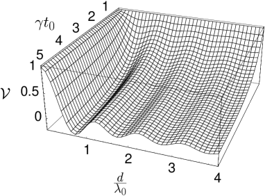
FIG. 6.: The function ${\cal V}$ in Eq. (91).

We now look at some particular cases. The intensity at the screen is displayed in Figure 7 for $d/\lambda_{0}=2$ and a few values of $\gamma t_{0}$. The quantity $|{\cal V}|$ is the visibility of the interference pattern

$$|{\cal V}|=\frac{I^{\prime}_{\rm max}-I^{\prime}_{\rm min}}{I^{\prime}_{\rm max}+I^{\prime}_{\rm min}}\ .$$ (92)

Roughly speaking, the visibility is related to the amplitude of the oscillations of the interference pattern and measures the degree of coherence of the interfering system [31]. Notice that the visibility decreases as $\gamma t_{0}$ is increased, namely when the emission process of the photon is faster. This is readily understood in terms of the discussion in Section 3 ($\lambda_{0}$ plays the role of $\lambda_{\rm L}$). The behavior of the visibility as a function of $d/\lambda_{0}$ is shown in Figure 8 for the same values of $\gamma t_{0}$ as those used in Figure 7.

In order to appreciate the meaning of these results, let us first observe that the interpretation of the visibility derives from (80): the first term in the r.h.s. of (91) is associated with those molecules that have not emitted any photon (and reach the screen in an excited state), while the second term is associated with those molecules that have emitted a photon before they hit the screen.

FIG. 7.: Intensity at the screen when $d/\lambda_{0}=2$, $X/\delta x(t_{0})=0.4$ and $\gamma t_{0}$ is varied. From top left to bottom right, $\gamma t_{0}=0,1,2,3$.

When the wavelength of the photon satisfies the coherence condition (42), $\lambda_{0}\gtrsim 2d$, by detecting the emitted photon we cannot extract any path information and the visibility reads

$${\cal V}\left(\gamma t_{0},\frac{d}{\lambda_{0}}\lesssim\frac{1}{2}\right)\simeq{\cal V}\left(\gamma t_{0},0\right)=1:$$ (93)

the interference pattern is equal to that obtained when no laser is present [namely, (90) reduces to (37)], irrespectively of the value of $\gamma t_{0}$.

FIG. 8.: The visibility of the interference pattern as a function of $d/\lambda_{0}$, for $\gamma t_{0}=0,1,2,3$.

Let now $\lambda_{0}<d$, so that the coherence condition (42) is not satisfied. We clearly see from Figure 8 that, somewhat unexpectedly, coherence is still largely preserved if $\gamma t_{0}\lesssim 1$, because even though the photon wavelength is small enough to yield information about the path of the interfering particle, such a path information is not accessible: it is, so to say, “stored” in the internal structure of the molecule. Such an information would be available to an external observer only if the photon were emitted. Mathematically,

$${\cal V}\left(\gamma t_{0},\frac{d}{\lambda_{0}}\gtrsim 1\right)\simeq{\cal V}\left(\gamma t_{0},\infty\right)=\exp(-\gamma t_{0})$$ (94)

which tends to vanish if the decay is rapid ($\gamma t_{0}\gg 1$) and to unity if the decay is slow ($\gamma t_{0}\ll 1$).

In conclusion, the interference pattern is blurred out (${\cal V}\simeq 0$), only if the photon emission process yields both a good resolution, $\lambda_{0}\lesssim d$, and a quick response, $\gamma t_{0}\gg 1$. We recover in this case the conclusions of the Heisenberg-Bohm microscope analyzed in Section 3: if the decay is rapid we have the situation shown in Figure 4(a), while if the decay is slower we are closer to the case depicted in Figure 4(b) [yielding the less stringent condition (44)]. Formally, the Heisenberg-Bohm microscope of Figure 4(a) is fully recovered in the (familiar) limit

$${\cal V}\left(\infty,\frac{d}{\lambda_{0}}\right)={\rm sinc}\left(\frac{2\pi d}{\lambda_{0}}\right).$$ (95)

It is interesting to notice that space and time considerations are both important in this context: in order to lose quantum coherence, the molecule must interact with its environment in such a way that its path information is not only available, but also quickly available. This is a significant difference with the Heisenberg-Bohm microscope: a good “resolution” is needed, both in space and time.

FIG. 9.: Intensity at the screen when $d/\lambda_{0}=0.84$, $X/\delta x(t_{0})=0.4$ and $\gamma t_{0}$ is varied. From top left to bottom right, $\gamma t_{0}=0,1,2,3$.

There is more. One might be led to think that the visibility (and therefore the quantum coherence) is always a decreasing function of $d/\lambda_{0}$: in other words, a smaller photon wavelength (yielding better path information) always increases decoherence. This expectation is incorrect: look at Figure 8, where the visibility exhibits in general an oscillatory behavior. “Regular” regions, where the visibility decreases by decreasing the wavelength, are interspersed with “anomalous” regions in which by decreasing the photon wavelength the visibility increases: a better microscope does not necessarily yield more information. One infers that there are physical situations in which the behavior of the visibility is somewhat “anomalous” and at variance with naive expectation. Similar cases were investigated in neutron optics [31] and are related to well-known phenomena in classical optics (see for instance Sec. 7.5.8 of Ref. [19]).

FIG. 10.: The visibility of the interference pattern as a function of $\gamma t_{0}$, for $d/\lambda_{0}=0.84$ (dashed line) and $2$ (continuous line). The former situation is “anomalous.”

The above discussion deals with spatial resolution. A similar phenomenon occurs also in time domain, where a faster photon emission (yielding path information) does not necessarily increase decoherence. In Figure 9 the intensity at the screen is shown for $d/\lambda_{0}=0.84$ and a few values of $\gamma t_{0}$. The visibility reaches a minimum (in fact vanishes) for $\gamma t_{0}=2$ and then increases again. (This phenomenon appears together with an interchange of minima and maxima.) Notice the difference with Figure 7. The behavior of the visibility for the cases shown in Figures 7 and 9 is displayed in Figure 10 as a function of $\gamma t_{0}$.

We conclude with an additional comment. For the numerical values considered in Section 2, one gets $X/\delta x(t_{0})=1.56$ and $\exp(-X^{2}/8\delta x^{2}(t_{0}))=0.74$, so that there are only a few oscillations within the envelope function, as can be seen in Figures 2 and 3. However, the assumptions leading to the expression (91) for the visibility [see the paragraph preceding (89)] maintain their validity. The interference patterns given by the approximate expression (90) and by the exact formulas (80)-(85) are shown in Figure 11: they are almost identical.

V A more refined picture of the molecule

A molecule of fullerene is a complicated object, that can absorb several visible photons at once and undergo quite involved processes in its internal structure. The physical model analyzed in the preceding section is too simple to describe such a rich physical picture. Although it yields nice insight, the model is unsatisfactory because it is not able to describe the absorption and reemission process of several photons. This is what one would need, because the physics of fullerene is for certain aspects related to that of a small black body, characterized by a well-defined temperature and in continuous interaction with its environment [25, 24, 23, 10].

FIG. 11.: Interference patterns for $X/\delta x(t_{0})=1.56$. The full line is the exact formula, obtained by (80)-(85), the dashed line the approximate expression (90). Compare with Figure 2.

It is possible to analyze the interference of fullerene by introducing a more realistic (and complicated) model: a detailed calculation is still feasible, but requires more sophisticated techniques and will be presented elsewhere. However, we will briefly outline some of the nice qualitative features of the physical picture that emerges from such an analysis.

The mesoscopic system (molecule of fullerene) can still be described by a model similar to the one introduced in the preceding section: the molecule is viewed as a multi-level system that starts its evolution, immediately after the slits, in a highly excited state (or possibly in a mixed state of given temperature). On its way to the screen, the molecule emits some (say $N=n\pm\triangle n$) photons of different energies and in random directions. Of course, unlike in the previous section, the photons have low energy, although the sum of their energies can be significant (and for instance comparable with the energy of the single photon emitted in the preceding section).

The question is: will the interference pattern be modified as a consequence of the multiple emission processes that take place between the slits and the screen? The answer is: less than one might think. In order to justify this statement at a semiquantitative level, look at Figure 12. The photons will be emitted in random directions and as a consequence the momentum of the molecule will recoil by the quantity

$$\triangle p\simeq\hbar\langle k\rangle\sqrt{n},$$ (96)

where $\hbar\langle k\rangle$ is the average momentum of the emitted photons and $n$ the average number of emitted photons. The molecule, as a consequence of light emission processes, loses a total energy $\triangle E\simeq n\hbar\langle k\rangle/c$ between the slits and the screen. However, according to (96), its momentum will only be changed by the quantity

$$\triangle p\simeq\frac{\triangle E}{c\sqrt{n}}.$$ (97)

For instance, the interference pattern will be only slightly affected by the emission of a large number of low-energy photons. This is an interesting qualitative conclusion.

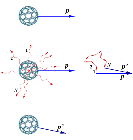
FIG. 12.: Random walk (96) in momentum space. $N$ (thermal) photons are emitted and the momentum of the molecule changes accordingly.

A more quantitative relation can be obtained by treating fullerene as a macroscopic system that emits thermal radiation at temperature $T$. The total intensity of emission $J_{0}$ and the total photon flux $\Phi_{0}$ emitted by a black body read [32]

$$J_{0} = \frac{cE}{4V}=\frac{\hbar}{4\pi^{2}c^{2}}\int_{0}^{\infty}d\omega\;\frac{\omega^{3}}{e^{\hbar\omega/k_{\rm B}T}-1}$$ (99)

$$=\frac{\pi^{2}}{60}\frac{k_{\rm B}^{4}}{c^{2}\hbar^{3}}T^{4},$$

$$\Phi_{0} = \frac{cN_{V}}{4V}=\frac{1}{4\pi^{2}c^{2}}\int_{0}^{\infty}d\omega\;\frac{\omega^{2}}{e^{\hbar\omega/k_{\rm B}T}-1}$$ (101)

$$=\frac{\zeta(3)}{2\pi^{2}}\frac{k_{\rm B}^{3}}{c^{2}\hbar^{3}}T^{3},$$

respectively, where $k_{\rm B}$ is the Boltzmann constant, $E$ ($N_{V}$) the total radiation energy (number of photons) contained in a cavity of volume $V$ and $\zeta(s)=\sum_{n=1}^{\infty}\frac{1}{n^{s}}$ the Riemann function ($\zeta(3)\simeq 1.202$). The energy and number of photons emitted by the surface $A$ of the fullerene molecule during its time of flight $t_{0}$ are, respectively,

$$\triangle E=J_{0}At_{0},\qquad n=\Phi_{0}At_{0}.$$ (102)

Therefore by making use of (102), (99) and (101), Eq. (97) reads

$$\triangle p \simeq \frac{J_{0}At_{0}}{c\sqrt{\Phi_{0}At_{0}}}=\kappa(At_{0})^{\frac{1}{2}}T^{\frac{5}{2}},$$ (103)

$$\kappa = \sqrt{\frac{2}{\zeta(3)}}\frac{\pi^{3}}{60}\frac{k_{\rm B}^{\frac{5}{2}}}{c^{2}\hbar^{\frac{3}{2}}}$$ (104)

$$= 4.85\times 10^{-24}\mbox{ kg / s${}^{\frac{3}{2}}$ K${}^{\frac{5}{2}}$}.$$ (105)

In agreement with Section 3, in order to observe interference, the transferred momentum $\triangle p$ must satisfy the inequality (coherence condition, obtained by (42) and (38))

$$\triangle p\lesssim\frac{h}{2d},$$ (106)

which translates into the following bound for the internal temperature $T$

$$T \lesssim \xi\frac{1}{(At_{0}d^{2})^{\frac{1}{5}}}\equiv T^{\prime}_{\rm dec}$$ (107)

$$\xi = \left(\frac{1800\;\zeta(3)}{\pi^{4}}\right)^{\frac{1}{5}}\frac{\hbar\;c^{\frac{4}{5}}}{k_{\rm B}}$$ (108)

$$= 8.59\times 10^{-5}\mbox{ K s${}^{\frac{1}{5}}$ m${}^{\frac{4}{5}}$}.$$ (109)

By taking $A=4\pi r^{2}=1.539\times 10^{-18}$m ($r\simeq 3.5$Å is the radius of a fullerene molecule) and $t_{0}=9.47$ms [12] we get

$$T^{\prime}_{\rm dec}\simeq 500\mbox{K}.$$ (110)

This bound is too strong: a fullerene molecule cannot be considered as an ordinary black body. Its curvature cannot be neglected [8, 10, 24] and its emitting surface is far from being flat. One can take a heuristic approach and summarize its behavior by multiplying the quantities in Eq. (102) by an emissivity coefficient $\alpha\simeq 4.5\cdot 10^{-5}$ (due to the curvature of the emitting surface for small atomic clusters [10]), to obtain

$$\triangle E=\alpha J_{0}At_{0},\qquad n=\alpha\Phi_{0}At_{0},$$ (111)

so that

$$\triangle p\simeq\sqrt{\alpha}\kappa(At_{0})^{\frac{1}{2}}T^{\frac{5}{2}},$$ (112)

This yields

$$T\lesssim\xi\alpha^{-\frac{1}{5}}\frac{1}{(At_{0}d^{2})^{\frac{1}{5}}}\equiv T_{\rm dec}.$$ (113)

This is a more reliable estimate, that should be valid at least as an order of magnitude. Equation (113) is a coherence condition. The quantity $T_{\rm dec}$ is the internal (“blackbody”) temperature of a fullerene molecule at which decoherent effects should become apparent in a double slit experiment. For the numerical values of the Vienna experiment [12, 25]

$$T_{\rm dec}\simeq 3700{\rm K}.$$ (114)

Notice that above $T\simeq 3000$K fullerene molecules begin to fragmentate (ionization is likely to occur at even lower temperatures). We are led to argue that the temperature of the fullerene molecule will only have a small influence on the visibility of the interference pattern, at least for the Vienna experimental configuration. However, if the experiment is modified by letting the fullerene go through an interferometer of the Mach-Zender type in order to increase the beam separation $d$ (say, up to a distance of order $1\mu$m), then intrinsic decoherence effects should come to light. The behavior of $T_{\rm dec}$ versus $d$ (slit separation) is shown in Figure 13 for a time of flight of 9.53ms (distance travelled $L=1.22$m and speed $v_{z}=128$m/s [12]). Decoherence effects should be visible at about 2000K for a beam separation of order of half a micron. (Notice: in such a situation, according to (111), the molecule emits $n\simeq 8.6$ photons.)

FIG. 13.: $T_{\rm dec}$ versus $d$ (slit separation) for a fullerene molecule. We set the time of flight $t_{0}=9.53$ms. The horizontal line is the temperature at which fragmentation becomes significant.

We stress that the calculation of this section is based on a heuristic model and is probably valid within a numerical factor of order unity. Indeed we have not considered a few effects that should yield interesting corrections: first, we have neglected the temperature of the environment (assuming that it is much lower than that of the molecule) and all cooling mechanisms of fullerene (which is a small black body and loses energy by emitting photons: since C₆₀ has 174 vibrational modes, 4 of which are infrared active, the temperature decrease during a time of flight of 10ms should be of a few hundreds Kelvin). Second, we have neglected all entanglement effects due to photon emissions into the environment (such entanglement effects were automatically taken into account in the calculation of the preceding section). Third, it should be emphasized that our calculation is valid for those fullerene molecules that reach the screen (detection system) in an electrically neutral state: the very hot C₆₀ molecules that yield C${}_{60}^{+}$ ions during the flight to the screen will strongly couple to environmental stray fields and will not interfere. Since the beautiful detection mechanism in the Vienna experiment hinges upon ionization, these additional ions should be removed from the beam. Fourth, fragmentation effects have not been considered. Finally, we notice that our estimate is based on the (conservative) approximation (106).

From a merely theoretical viewpoint, it is interesting to observe how one obtains sensible results in the mesoscopic domain by combining thermodynamical considerations with a pure quantum mechanical analysis.

VI What is decoherence?

Decoherence is an interesting phenomenon. Although the quantum mechanical coherence is readily defined and is intuitively related to the possibility of creating a superposition in a Hilbert space, it is not obvious what the lack of quantum coherence is. Most physicist would say that such a lack of coherence can be given a meaning only in a statistical sense (but there are noteworthy historical exceptions [33]).

However, without endeavoring to give rigorous definitions, one has the right to ask when, how and why coherence is maintained. This is not an easy question, in particular if the system investigated is not strictly microscopic. In this paper we have studied a molecule with an increasingly complicated internal structure. If the molecule is “elementary,” i.e. structureless, the usual description in terms of the Heisenberg-Bohm microscope applies and interference is lost when a photon of suitable wavelength is scattered off the molecule after the latter has gone through a double slit. If, on the other hand, the molecule can be reasonably schematized as a two-level system, the situation is not that simple. One still needs a photon of suitable wavelength to destroy interference, but in addition the photon reemission process must be rapid. If, for instance, the photon is reemitted only after the molecule has reached the screen, no Welcher Weg information is available and interference (coherence) is preserved. In words, the two-level system needs a certain time to “explore” its environment, e.g. via photon emission, and “give away” Welchew Weg information. Note: via photon emission, not photon absorption!

If the picture becomes more complicated and the molecule can absorb and reemit a large number of photons, then the situation becomes even more interesting. In such a case the molecule might be complicated enough to have an internal temperature and one can properly talk of “mesoscopic interference.” In such a situation, the mesoscopic system will slowly “explore” its environment by emitting photons in the course of its evolution and its branch waves will slowly “decohere” (namely, their momentum will recoil due to repeated photon emissions and their states propagating through different slits will get entangled with increasingly orthogonal states of the electromagnetic field, that plays the role of environment). In this sense, coherence (viewed as ability to interfere) simply means isolation from the environment—a lesson that experimental physicists know much better (and since much longer) than their theoretical colleagues, who do not (and never had to) care about “isolating” a beam in order to make it interfere.

We notice that there is no big conceptual change if the molecule reemits an electron, rather than a photon, after a certain characteristic (life)time due to internal rearrangements. For example, ions C${}_{60}^{+}$ are quickly produced after multiphoton excitation with laser pulses, for wavelengths ranging from ultraviolet (200 nm) to infrared (1000 nm) light. (It is just this emission process of an electron with well-defined energy [8, 23] that was brilliantly used to detect the fullerene molecules in [11, 25].) Electron emission gives rise to nonnegligible recoil and therefore the interference pattern will vanish upon averaging over the emission direction. More so, coupling to stray electric field would prevent any reasonable isolation of C${}_{60}^{+}$ from the environment.

We are left with an interesting question, though. When can a system be described by a wave function? When is a quantum state “pure”? The experiment [11] has taught us something fundamental. If a good experimentalist can isolate the internal degrees of freedom of a (microscopic, mesoscopic or even macroscopic) system and at the same time succeeds in controlling the coherent superposition of an additional dynamical variable (say, the coordinate of the center of mass of the molecule) then the state

superposed wave function $$\times$$ internal state

will interfere (we apologize for the abuse of notation and additional inaccuracies). Notice that the internal state can be mixed and can even be a black body. If there were a party (with a few cats) going on inside the fullerene molecule and if the external world would not be able to notice, not even in principle, the molecule would still interfere. Flabbergasting.

A The Weisskopf-Wigner approximation and the Fermi “golden” rule

We study here the evolution of the system introduced in Section 4 and derive Eqs. (58)-(62). The initial state is (55) and the evolution reads

$$|\Psi_{\rm tot}(t)\rangle=e^{-iH_{0}t/\hbar}U_{I}(t)|\Psi_{\rm tot}\rangle=e^{-iH_{0}t/\hbar}|\Psi_{\rm tot}(t)\rangle_{I},$$ (A.1)

with

$$U_{I}(t) = T\exp\left(-\frac{i}{\hbar}\int_{0}^{t}d\tau\;V_{I}(\tau)\right),$$ (A.2)

$$V_{I}(\tau) = e^{iH_{0}\tau/\hbar}Ve^{-iH_{0}\tau/\hbar},$$ (A.3)

where $I$ denotes the interaction picture and $T$ time ordering. We study the emission process by solving the Schrödinger equation in the interaction picture

$$|\dot{\Psi}_{\rm tot}(t)\rangle_{I}=-\frac{i}{\hbar}V_{I}(t)|\Psi_{\rm tot}(t)\rangle_{I}.$$ (A.4)

In the notation of Section 4, the interaction Hamiltonian is

$$V_{I}(t)\! = \!\sum_{i}\left[\Phi_{i}e^{-i\left(\omega_{i}-\frac{\hbar k_{i}^{2}}{2m}-\omega_{0}\right)t}e^{i\mbox{\boldmath$k$}_{i}\cdot\mbox{\boldmath$x$}}e^{i\frac{\mbox{\boldmath$k$}_{i}\cdot\mbox{\boldmath$p$}}{m}\;t}|e\rangle\langle g|a_{i}\right.$$ (A.6)

$$\quad\quad+\mbox{h.c.}\Bigg{]}$$

and by writing the state of the system as

$$|\Psi_{\rm tot}(t)\rangle_{I} = \alpha(t)|e^{i\mbox{\boldmath$k$}_{\rm L}\cdot\mbox{\boldmath$x$}}\Psi_{0},e,0\rangle$$ (A.9)

$$+\sum_{i}\beta_{i}(t)e^{i\left(\delta_{i}-\frac{\hbar k_{i}^{2}}{2m}\right)t}$$

$$\times|e^{-i\frac{\mbox{\boldmath$k$}_{i}\cdot\mbox{\boldmath$p$}}{m}\;t}e^{i(\mbox{\boldmath$k$}_{\rm L}-\mbox{\boldmath$k$}_{i})\cdot\mbox{\boldmath$x$}}\Psi_{0},g,1_{i}\rangle,\qquad$$

with

$$\delta_{i}=\frac{\hbar\mbox{\boldmath$k$}_{i}}{m}\cdot(\mbox{\boldmath$k$}_{0}+\mbox{\boldmath$k$}_{\rm L})-\frac{\hbar k_{i}^{2}}{2m},$$ (A.10)

the Schrödinger equation (A.4) reads

$$\dot{\alpha} = -\frac{i}{\hbar}\sum_{i}\beta_{i}(t)\Phi_{i}e^{-i(\bar{\omega}_{i}-\omega_{0})t},$$ (A.11)

$$\dot{\beta}_{i} = -\frac{i}{\hbar}\alpha(t)\Phi_{i}^{*}e^{i(\bar{\omega}_{i}-\omega_{0})t},$$ (A.12)

where $\bar{\omega}_{i}=\omega_{i}-\delta_{i}$. Incorporating the initial conditions $\alpha(0)=1$, $\beta_{i}(0)=0$, Eqs. (A.12) are formally solved to yield

$$\dot{\alpha}(t) = -\sum_{i}\frac{|\Phi_{i}|^{2}}{\hbar^{2}}\int_{0}^{t}d\tau\;e^{-i(\bar{\omega}_{i}-\omega_{0})\tau}\alpha(t-\tau).$$ (A.13)

$$\beta_{i}(t) = -\frac{i}{\hbar}\Phi_{i}^{*}\int_{0}^{t}d\tau\;e^{i(\bar{\omega}_{i}-\omega_{0})\tau}\alpha(\tau),$$ (A.14)

The former is an integro-differential equation for $\alpha(t)$ and can be rewritten in the form

$$\dot{\alpha}(t)=-\int_{0}^{t}d\tau\;\sigma(\tau)\alpha(t-\tau),$$ (A.15)

where $\sigma(t)$ is the Fourier transform of the form factor $\Gamma(\omega)$

$$\sigma(t) = \int\frac{d\omega}{2\pi}\;\Gamma(\omega)e^{-i(\omega-\omega_{0})t},$$ (A.16)

$$\Gamma(\omega) = \frac{2\pi}{\hbar^{2}}\sum_{i}|\Phi_{i}|^{2}\delta(\bar{\omega}_{i}-\omega).$$ (A.17)

If $\Gamma(\omega)$ is a smooth function with bandwidth $\Lambda$, by the uncertainty relation $\triangle t\triangle\omega\simeq 1$, $\sigma(t)$ is significantly different from zero only within a time interval $\tau_{c}\simeq 1/\Lambda$. Therefore, the integral in the r.h.s. of Eq. (A.15) takes a substantial contribution only from the time domain $(0,\tau_{c})$, as shown in Figure 14.

FIG. 14.: The functions $\alpha$ and $\sigma$.

If we assume that the evolution of $\alpha(t)$ takes place on a time scale that is much longer than $\tau_{c}$, we get $\alpha(t-\tau)\simeq\alpha(t)$ for $\tau\lesssim\tau_{c}$, whence

$$\dot{\alpha}(t)\simeq-\alpha(t)\int_{0}^{t}d\tau\;\sigma(\tau).$$ (A.18)

At times $t\gg\tau_{c}$, the integral becomes almost independent of $t$, the integration can be extended up to $t=+\infty$ and we obtain from (A.16)

$$\int_{0}^{t}d\tau\;\sigma(\tau)\simeq\int_{0}^{\infty}d\tau\int\frac{d\omega}{2\pi}\;\Gamma(\omega)e^{-i(\omega-\omega_{0}-i0^{+})\tau},$$ (A.19)

where we introduced an infinitely small negative imaginary term $-i0^{+}$ in order to assure the convergence. By interchanging the order of integration, we get

$$\int\frac{d\omega}{2\pi}\;\Gamma(\omega)\int_{0}^{\infty}d\tau e^{-i(\omega-\omega_{0}-i0^{+})\tau}$$ (A.20)

$$=\int\frac{d\omega}{2\pi}\;\Gamma(\omega)\frac{-i}{\omega-\omega_{0}-i0^{+}},$$ (A.21)

which, by making use of the well-known formula

$$\lim_{\epsilon\rightarrow 0^{+}}\frac{1}{x-i\epsilon}={\cal P}\frac{1}{x}+i\pi\delta(x),$$ (A.22)

where ${\cal P}$ denotes the principal part, becomes

$$\int_{0}^{t}d\tau\;\sigma(\tau)\simeq i\Delta+\frac{\gamma}{2},$$ (A.23)

$$\Delta = {\cal P}\int\frac{d\omega}{2\pi}\;\frac{\Gamma(\omega)}{\omega_{0}-\omega}={\cal P}\sum_{i}\frac{|\Phi_{i}|^{2}/\hbar^{2}}{\omega_{0}-\bar{\omega}_{i}},\;\;\;\;$$ (A.24)

$$\gamma = \Gamma(\omega_{0})=\frac{2\pi}{\hbar^{2}}\sum_{i}|\Phi_{i}|^{2}\delta(\bar{\omega}_{i}-\omega_{0}).$$ (A.25)

The last two quantities are the second-order correction to the energy $\hbar\omega_{0}$ and the Fermi “golden” rule [30], Eq. (61) in the text. By plugging Eq. (A.23) into Eq. (A.18) we finally get

$$\dot{\alpha}(t)=-\left(i\Delta+\frac{\gamma}{2}\right)\alpha(t),$$ (A.26)

which is the celebrated Weisskopf-Wigner approximation [27, 28]. It simply consists in replacing a complex dynamics with memory effects [Eq. (A.15)] with a simpler one characterized by a purely Markovian equation (A.26), giving rise to exponential decay

$$\alpha(t)=\exp\left(-i\Delta t-\frac{\gamma}{2}t\right).$$ (A.27)

As we stressed before, this replacement is justified for $t\gg\tau_{c}$ only if there exist two well separated time scales, i.e. only if the amplitude probability $\alpha(t)$ of the excited level $|e\rangle$ evolves much more slowly than the characteristic time $\tau_{c}$ of the photon reservoir. By making use of Eq. (A.27) and the definitions (A.24)-(A.25) this condition translates into the following inequality

$$\Delta^{-1},\gamma^{-1}\gg\tau_{c}\quad\Leftrightarrow\quad\Gamma(\omega_{0})\ll\Lambda,$$ (A.28)

which is always verified for sufficiently small coupling and/or large bandwidth $\Lambda$, such as QED decay processes in vacuum [remember that $\Gamma(\omega)\propto|\Phi|^{2}\propto\;$(coupling constant)²].

By substituting the solution (A.27) in the second equation (A.14) and performing the integration, one gets

$$\beta_{i}(t)=\frac{\Phi^{*}_{i}}{\hbar}\frac{1-e^{i(\bar{\omega}_{i}-\omega_{0}-\Delta)t-\gamma t/2}}{\bar{\omega}_{i}-\omega_{0}-\Delta+i\gamma/2},$$ (A.29)

which is Eq. (62) of the text. By plugging (A.27) and (A.29) into (A.9) and using (A.1) one gets Eq. (58) of the text. In our analysis we will always neglect the energy shift $\hbar\Delta$ or, equivalently, absorb it into the (renormalized) free energy $\hbar\omega_{0}$. We will also neglect the phase shift $\delta_{i}$, which is due to recoil and Doppler effects. Indeed both terms in (A.10) are much smaller than the transition frequency $\omega_{0}$: $(\hbar k^{2}_{i}/2m)/\omega_{0}\sim\hbar\omega_{0}/2mc^{2}\ll 1$ and $(\hbar\mbox{\boldmath$k$}\cdot\mbox{\boldmath$k$}_{0}/m)/\omega_{0}\sim v_{z}/c\ll 1$. Moreover, note that when we write the evolved state $|\Psi_{\rm tot}(t)\rangle_{I}$ as in Eq. (A.9) we are neglecting any contributions out of the relevant Tamm-Duncoff sector, due to frequency-dependent Doppler and/or recoil effects, which deform the Gaussian wave packet.

B Evaluation of an integral

We want to derive Eq. (82). We start by computing the integral

$$\sum_{i}|\beta_{i}(t)|^{2}=\sum_{i}\frac{|\Phi_{i}|^{2}}{\hbar^{2}}\;\frac{|1-e^{i(\omega_{i}-\omega_{0})t-\gamma t/2}|^{2}}{(\omega_{i}-\omega_{0})^{2}+\gamma^{2}/4}.$$ (B.1)

This is an interesting integral (often left as an exercise in good textbooks [29]), that must be performed, like other calculations related to the Fermi “golden” rule, with the help of physical intuition. Expanding the square we find

$$\sum_{i}\frac{|\Phi_{i}|^{2}}{\hbar^{2}}\;\frac{1+e^{-\gamma t}-2e^{-\gamma t/2}\cos(\omega_{i}-\omega_{0})t}{(\omega_{i}-\omega_{0})^{2}+\gamma^{2}/4}$$ (B.2)

$$=(1+e^{-\gamma t})\sum_{i}\frac{|\Phi_{i}|^{2}/\hbar^{2}}{(\omega_{i}-\omega_{0})^{2}+\gamma^{2}/4}$$ (B.3)

$$\quad-2e^{-\gamma t/2}\sum_{i}\frac{|\Phi_{i}|^{2}}{\hbar^{2}}\frac{\cos(\omega_{i}-\omega_{0})t}{(\omega_{i}-\omega_{0})^{2}+\gamma^{2}/4}$$ (B.4)

$$=1+e^{-\gamma t}-2e^{-\gamma t/2}\sum_{i}\frac{|\Phi_{i}|^{2}}{\hbar^{2}}\frac{\cos(\omega_{i}-\omega_{0})t}{(\omega_{i}-\omega_{0})^{2}+\gamma^{2}/4},$$ (B.5)

(B.6)

where the Fermi “golden” rule (A.25)

$$\gamma=\frac{2\pi}{\hbar^{2}}\sum_{i}|\Phi_{i}|^{2}\delta(\omega_{i}-\omega_{0})$$ (B.7)

has been used. Moreover, we obtain

$$\int dx\frac{\cos xt}{x^{2}+\gamma^{2}/4}=\int dx\frac{e^{ixt}}{x^{2}+\gamma^{2}/4}\\ =\frac{2\pi}{\gamma}e^{-\gamma t/2},$$ (B.8)

so that, in the spirit of the golden rule,

$$\frac{\cos xt}{x^{2}+\gamma^{2}/4}\stackrel{{\scriptstyle\gamma\to 0}}{{\sim}}\frac{2\pi}{\gamma}e^{-\gamma t/2}\delta(x).$$ (B.9)

Plugging this result into Eq. (B.6) we get

$$\sum_{i}|\beta_{i}(t)|^{2}=1-e^{-\gamma t}.$$ (B.10)

We can now tackle Eq. (82). This appears in the form

$$\sum_{i}|\beta_{i}(t)|^{2}f_{i}$$ (B.11)

$$=(1+e^{-\gamma t})\frac{2\pi}{\gamma}\sum_{i}\frac{|\Phi_{i}|^{2}}{\hbar^{2}}f_{i}\delta(\omega_{i}-\omega_{0})$$ (B.12)

$$\quad-2e^{-\gamma t/2}\frac{2\pi}{\gamma}e^{-\gamma t/2}\sum_{i}\frac{|\Phi_{i}|^{2}}{\hbar^{2}}f_{i}\delta(\omega_{i}-\omega_{0})$$ (B.13)

$$=(1-e^{-\gamma t})\frac{2\pi}{\gamma}\sum_{i}\frac{|\Phi_{i}|^{2}}{\hbar^{2}}f_{i}\delta(\omega_{i}-\omega_{0}).\quad$$ (B.14)

The above derivation applies under the same conditions of Appendix A, namely when $\gamma\ll$ bandwidth. Now consider the average of Eq. (B.14) over the direction of the molecular dipole $d$

$$\left\langle\sum_{i}|\beta_{i}(t)|^{2}f_{i}\right\rangle=\sum_{i}\left\langle|\beta_{i}(t)|^{2}\right\rangle f_{i}$$ (B.15)

$$\;\;=(1-e^{-\gamma t})\frac{2\pi}{\gamma}\sum_{i}\frac{\left\langle|\Phi_{i}|^{2}\right\rangle}{\hbar^{2}}f_{i}\delta(\omega_{i}-\omega_{0}).\qquad$$ (B.16)

Note that

$$\left\langle|\Phi_{i}|^{2}\right\rangle = \frac{e^{2}\hbar\omega_{i}}{2\epsilon_{0}L^{3}}\frac{1}{4\pi}\int d\Omega_{\mbox{\boldmath$d$}}|\mbox{\boldmath$d$}\cdot\mbox{\boldmath$\epsilon$}_{i}|^{2}$$ (B.17)

$$= \frac{e^{2}\hbar\omega_{i}}{2\epsilon_{0}L^{3}}\frac{1}{3}|\mbox{\boldmath$d$}|^{2}$$ (B.18)

is only a function of $\omega_{i}$ and does not depend on the direction of the photon momentum $\mbox{\boldmath$k$}_{i}$, whence

$$\left\langle\sum_{i}|\beta_{i}(t)|^{2}f_{i}\right\rangle$$ (B.19)

$$\;\;=(1-e^{-\gamma t})\frac{2\pi}{\gamma}\frac{e^{2}\omega_{0}|\mbox{\boldmath$d$}|^{2}}{6\hbar\epsilon_{0}L^{3}}\sum_{i}f_{i}\delta(\omega_{i}-\omega_{0})$$ (B.20)

$$\;\;=(1-e^{-\gamma t})\frac{\pi^{2}c^{3}}{\omega_{0}^{2}L^{3}}\sum_{i}f_{i}\delta(\omega_{i}-\omega_{0}).\qquad$$ (B.21)

In the continuum limit, if $f_{i}$ does not depend on the photon polarization $\lambda$, we finally get

$$\left\langle\sum_{i}|\beta_{i}(t)|^{2}f_{i}\right\rangle$$ (B.22)

$$\;\;=(1-e^{-\gamma t})\frac{c^{3}}{\omega_{0}^{2}4\pi}\int d^{3}k\;f_{\mbox{\boldmath$k$}}\delta(\omega-\omega_{0})$$ (B.23)

$$\;\;=(1-e^{-\gamma t})\frac{1}{4\pi}\int d\Omega_{\mbox{\boldmath$\bar{k}$}}\;f_{\mbox{\boldmath$\bar{k}$}},\qquad$$ (B.24)

with $|\mbox{\boldmath$\bar{k}$}|=\omega_{0}/c$, which yields the result we sought.

REFERENCES

- [1] Feynman, R.P., Leighton, R.B., and Sands, M. 1965, The Feynman Lectures on Physics, Volume III, Addison Wesley, Reading, Massachusetts.
- [2] Mandel, L. and Wolf, E. 1995, Optical Coherence and Quantum Optics, Cambridge University Press, Cambridge.
- [3] Rauch, H. and Werner, S.A. 2000, Neutron Interferometry: Lessons in Experimental Quantum Mechanics, Oxford University Press, Oxford.
- [4] Tonomura, A. 1994, Electron Holography, Springer, Heidelberg.
- [5] Carnal, O. and Mlynek, J. 1991, Phys. Rev. Lett. 66, 2689.
- [6] Schöllkopf, W. and Toennies, J.P. 1994, Science 266, 1345.
- [7] Chapman, M.S., Ekstrom, C.R., Hammond, T.D., Rubenstein, R.A., Schmiedmayer, J., Wehinger, S. and Pritchard, D.E. 1995, Phys. Rev. Lett. 74, 4783.
- [8] Ding, D. et al 1994, Phys. Rev. Lett. 73, 1084.
- [9] Mitzner, R. and Campbell, E.E.B. 1995, J. Chem. Phys. 103, 2445.
- [10] Kolodney, E., Budrevich, A. and Tsipinyuk, B. 1995, Phys. Rev. Lett. 74, 510.
- [11] Arndt, M., Nairz, O., Voss-Andreae, J., Keller, C., van der Zouw, G. and Zeilinger, A. 1999, Nature 401, 680.
- [12] Arndt, M., Nairz, O., Petschinka J. and Zeilinger, A. 2001, C.R. Acad. Sci. Paris, t.2 S rie IV, 1.
- [13] Gould, S.J. 1989, Wonderful life. The Burgess Shale and the Nature of History, W.W. Norton & Company, New York.
- [14] Heisenberg, W. 1949, The Physical Principles of the Quantum theory, Dover, New York.
- [15] Dirac, P.A.M. 1958, The Principles of Quantum Mechanics, Oxford Univ. Press, London;
- [16] Feynman, R.P. and Hibbs, G. 1965, Quantum mechanics and Path Integrals, McGraw-Hill, New York.
- [17] Scully, M.O., Englert, B. and Schwinger, J. 1989, Phys. Rev. A40, 1775.
- [18] Bohm, D. 1951, Quantum Theory, Dover, New York.
- [19] Born, M. and Wolf, E. 1999, Principles of Optics, Cambridge University Press, Cambridge.
- [20] Zeilinger, A., Gähler, R., Shull, C.G., Treimer, W. and Mampe, W. 1988, Rev. Mod. Phys. 60, 1067.
- [21] Grisenti, R.E., Schöllkopf, W., Toennies, J.P., Hegerfeldt, G.C. and Köhler, T. 1999, Phys. Rev. Lett. 83, 1755.
- [22] Wheeler, J.A. 1978, in Mathematical Foundations of Quantum Theory, Ed. R. Marlow, Academic Press, New York, p. 9.
- [23] Hansen, K. and Echt, O. 1997, Phys. Rev. Lett. 78, 2337.
- [24] Hansen, K. and Campbell, E.E.B. 1998, Phys. Rev. E58, 5477.
- [25] Nairz, O., Arndt, M. and Zeilinger, A. 2000, J. Mod. Opt. 47, 2811.
- [26] Cohen-Tannoudji, C., Dupont-Roc, J. and Grynberg, G. 1992 Atom-Photon Interactions, Wiley & Sons, New York.
- [27] Weisskopf, V. and Wigner, E.P. 1930, Z. Phys. 63, 54; 65, 18.
- [28] Breit G. and Wigner, E.P. 1936, Phys. Rev. 49, 519.
- [29] Merzbacher, E. 1961, Quantum mechanics, Wiley & Sons, New York.
- [30] Fermi, E. 1932, Rev. Mod. Phys. 4, 87; 1950, Nuclear Physics, Univ. Chicago, Chicago, pp. 136, 148; See also 1960, Notes on Quantum Mechanics. A Course Given at the University of Chicago in 1954, edited by E Segré, Univ. Chicago, Chicago, Lec. 23.
- [31] Facchi, P., Mariano, A. and Pascazio, S. 2001, Phys. Rev. A63, 052108.
- [32] Landau, L.D. and Lifshitz, E.M. 1997, Statistical Physics, Part I, Butterworth-Heinemann, Oxford.
- [33] Namiki, M., Pascazio, S. and Nakazato, H. 1997, Decoherence and Quantum Measurements, World Scientific, Singapore.