Interferometric Bell-state preparation using femtosecond-pulse-pumped Spontaneous Parametric Down-Conversion

Abstract

We present theoretical and experimental study of preparing maximally entangled two-photon polarization states, or Bell states, using femtosecond pulse pumped spontaneous parametric down-conversion (SPDC). First, we show how the inherent distinguishability in femtosecond pulse pumped type-II SPDC can be removed by using an interferometric technique without spectral and amplitude post-selection. We then analyze the recently introduced Bell state preparation scheme using type-I SPDC. Theoretically, both methods offer the same results, however, type-I SPDC provides experimentally superior methods of preparing Bell states in femtosecond pulse pumped SPDC. Such a pulsed source of highly entangled photon pairs is useful in quantum communications, quantum cryptography, quantum teleportation, etc.

I Introduction

The nature of quantum entanglement attracted a great deal of attention even in the early days of quantum mechanics, yet it remained an unsolvable subject of philosophy until Bell showed the possibility of practical experimental tests [1, 2, 3, 4]. Since then, many experimental tests on the foundations of quantum mechanics have been performed [5, 6, 7, 8]. All these tests confirmed quantum mechanical predictions. More recently, experimental and theoretical efforts are being shifted to “applications”, such as quantum communications, quantum cryptography [9], and quantum teleportation [10], taking advantage of the peculiar physical properties of quantum entanglement. It is clear that preparation of maximally entangled two-particle (two-photon) entangled states, or Bell states, is an important subject in modern experimental quantum optics.

By far the most efficient source of obtaining two-particle entanglement is spontaneous parametric down-conversion (SPDC). SPDC is a nonlinear optical process in which a higher-energy pump photon is converted into two lower-energy daughter photons, usually called the signal and the idler, inside a non-centrosymmetric crystal [11]. In type-I SPDC, both daughter photons have the same polarizations but in type-II SPDC, the signal and the idler photons have orthogonal polarizations. The signal and the idler are generated into a non-factorizable entangled state. The photon pair is explicitly correlated in energy and momentum or equivalently in space and time. To prepare a maximally entangled two-photon polarization state, or a Bell state, one has to make appropriate local operations on the SPDC photon pairs.

The polarization Bell states, for photons, can be written as

$$|\Phi^{\pm}\rangle = |X_{1},X_{2}\rangle\pm|Y_{1},Y_{2}\rangle,$$ (1)

$$|\Psi^{\pm}\rangle = |X_{1},Y_{2}\rangle\pm|Y_{1},X_{2}\rangle,$$ (2)

where the subscripts 1 and 2 refer to two different photons, photon 1 and photon 2, respectively, and they can be arbitrarily far apart from each other. $|X\rangle$ and $|Y\rangle$ form the orthogonal basis for the polarization states of a photon, for example, it can be horizontal ( $|H\rangle$) and vertical ($|V\rangle$) polarization state, as well as $|45^{\circ}\rangle$ and $|-45^{\circ}\rangle$, respectively.

The subject of this paper is a detailed theoretical and experimental account of how one can prepare a polarization Bell state using femtosecond pulse pumped SPDC. In section I, we discuss why one needs such a pulsed source of Bell states, what happens when femtosecond pulsed laser is used to pump a type-II SPDC, and what has been done to recover the visibility in femtosecond pulse pumped type-II SPDC. In section II, we present a detailed theoretical description of how one can prepare a polarization Bell state using femtosecond pulse pumped type-II SPDC without any post-selection, followed by the experiment in section III. We then turn our attention to type-I SPDC and investigate it in detail theoretically in section IV and experimentally in section V.

The quantum nature of SPDC was first studied by Klyshko in late 1960’s [12]. Zel’dovich and Klyshko predicted the strong quantum correlation between the photon pairs in SPDC [13], which was first experimentally observed by Burnham and Weinberg [14]. The nonclassical properties of SPDC were first applied to develop an optical brightness standard [15] and absolute measurement of detector quantum efficiency [16].

Quantum interference effect in SPDC was first clearly demonstrated by Hong, Ou, and Mandel [17]. Shih and Alley first used SPDC to prepare a Bell state [7]. Such experiments have used type-I non-collinear SPDC and a beamsplitter to superpose the signal-idler amplitudes. Experimentally, type-I non-collinear SPDC is not an attractive way of preparing a Bell state mostly due to the difficulties involved in alignment of the system. Collinear type-II SPDC developed by Shih and Sergienko resolved this issue [18]. There is, however, a common problem: the entangled photon pairs have 50% chances of leaving at the same output ports of the beamsplitter. Therefore, the state prepared after the beamsplitter may not be considered as a Bell state without amplitude post-selection as pointed out by De Caro and Garuccio [19]. Only when one considers the coincidence contributing terms by throwing away two out of four amplitudes (post-selection of 50% of the amplitudes), the state is then considered to be a Bell state. Kwiat et al solved this problem by using non-collinear type-II SPDC [20]. This non-collinear type-II SPDC method of preparing a Bell state has been widely used in quantum optics community.

Recently, cw pumped type-I SPDC has also been used to prepare Bell states. Kwiat et al used two thin nonlinear crystals to prepare Bell states using non-collinear type-I SPDC [21] and Burlakov et al used a beamsplitter to join collinear type-I SPDC from two thick crystals in a Mach-Zehnder interferometer type setup [22].

Therefore, in cw pumped SPDC, there are readily available well-developed methods of preparing a Bell state. However, entangled photon pairs occur randomly within the coherence length of the pump laser beam. This huge time uncertainty makes it difficult to use in some applications, such as generation of multi-photon entangled state, quantum teleportation, etc, as interactions between entangled photon pairs generated from different sources are required. This difficulty was thought to be solved by using a femtosecond pulse laser as a pump. Unfortunately, femtosecond pulse pumped type-II SPDC shows poor quantum interference visibility due to the very different (compared to the cw case) behavior of the two-photon effective wave-function [23]. One has to utilize special experimental schemes to maximize the overlap of the two-photon amplitudes. Traditionally, the following methods were used to restore the quantum interference visibility in femtosecond pulse pumped type-II SPDC: (i) to use a thin nonlinear crystal ($\leq 100\mu$m) [24] or (ii) to use narrow-band spectral filters in front of detectors [25]. Both methods, however, reduce the available flux of the entangled photon pair significantly and cannot achieve complete overlap of the wave-functions in principle. We will discuss this in detail in section II.

Branning et al first reported an interferometric technique to remove the intrinsic distinguishability in femtosecond pulse pumped type-II SPDC without using narrowband filters and a thin crystal [26]. This method, however, cannot be used to prepare a Bell state since four biphoton amplitudes are involved in the quantum interference process [27]. This issue will be discussed in section II. More recently, Atatüre et al. claimed recovery of high-visibility quantum interference in pulse pumped type-II SPDC from a thick crystal without spectral post-selection. Unfortunately, the theory as well as the interpretation of the experimental data presented their work are shown to be in error [29]. Then it is fair to say that there have been no generally accepted method of preparing a Bell state from femtosecond pulse pumped SPDC without making any post-selection, especially the spectral post-selection. In the following sections, we will present experimental studies of preparing a Bell state using femtosecond pulse pumped SPDC (both type-II and type-I) together with the theoretical analysis.

II Bell state preparation using type-II SPDC: Theory

Let us first briefly discuss the basic formalism of pulse pumped type-II SPDC as discussed by Keller and Rubin [23]. A femtosecond pulse pumps a type-II BBO crystal to create entangled photon pairs via SPDC process. Orthogonally polarized signal and idler photons are separated by a polarizing beam splitter (PBS) and detected by two detectors, see Fig.1(a).

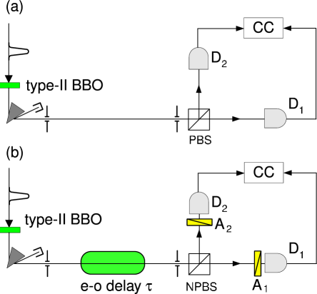
FIG. 1.: (a) Most simple two-photon correlation experiment. A femtosecond pulse pumps a type-II BBO crystal to create entangled photon pairs via SPDC process. Orthogonally polarized signal and idler photons are separated by a polarizing beam splitter ($PBS$) and detected by two detectors $D_{1}$ and $D_{2}$. (b) Collinear Hong-Ou-Mandel interferometer to observe quantum interference. The e-o delay $\tau$ can be introduced by a stack of quartz plates. $NPBS$ is a 50/50 non-polarizing beam splitter. $A_{1}$ and $A_{2}$ are polarization analyzers.

Let us start from the Hamiltonian of the SPDC [23, 30]

$${\mathcal{H}}=\epsilon_{0}\int d^{3}\vec{r}\chi^{(2)}E_{p}(z,t)E_{o}^{(-)}E_{e}^{(-)},$$ (3)

where $E_{p}(z,t)$ is the electric field for the pump pulse which is considered to be classical, and $E_{o}^{(-)}$ ($E_{e}^{(-)}$) is the negative frequency part of the quantized electric field for the $o$-polarized ($e$-polarized) photon inside the $\chi^{(2)}$ nonlinear crystal (BBO). The pump field can be written as

$$E_{p}(z,t)={\mathcal{E}}_{p}\int d\omega_{p}e^{-[\omega_{p}-\Omega_{p}]^{2}/\sigma_{p}^{2}}e^{i[k_{p}(\omega_{p})z-\omega_{p}t]},$$ (4)

where ${\mathcal{E}}_{p}$ is the amplitude of the pump pulse, $\Omega_{p}$ is the central frequency of the pump pulse, $\sigma_{p}^{2}=4\ln 2/[\sigma^{\rm FWHM}_{p}]^{2}$ where $\sigma^{\rm FWHM}_{p}$ is the FWHM bandwidth of the pump pulse, and $z$-direction is taken to be the pump pulse propagation direction. In the interaction picture, the state of SPDC is calculated from first-order perturbation theory [30]

$$|\psi\rangle = -\frac{i}{\hbar}\int_{-\infty}^{\infty}dt{\mathcal{H}}|0\rangle,$$ (5)

$$= C\int dk_{o}dk_{e}d\omega_{p}\int_{o}^{L}dze^{-[\omega_{p}-\Omega_{p}]^{2}/\sigma_{p}^{2}}e^{i\Delta z}$$ (7)

$$\times\delta(\omega_{o}+\omega_{e}-\omega_{p})a_{o}^{\dagger}a_{e}^{\dagger}|0\rangle,$$

where $C$ is a constant, $L$ is the thickness of the crystal, $a_{o}^{\dagger}$ ($a_{e}^{\dagger}$) is the creation operator of $o$-polarized ($e$-polarized) photon in a given mode, and $\Delta=k_{p}-k_{o}-k_{e}$ the phase mismatch.

The state vector $|\psi\rangle$ obtained in Eq.(7) is used to calculate the probability of getting a coincidence count [31].

$$R_{c}\propto\int dt_{1}\int dt_{2}|\langle 0|E_{2}^{(+)}E_{1}^{(+)}|\psi\rangle|^{2},$$ (8)

where the field at the detector $D_{1}$ can be written as

$$E_{1}^{(+)}=\int d\omega^{\prime}e^{-[\omega^{\prime}-\Omega_{1}]^{2}/\sigma_{1}^{2}}e^{-i\omega^{\prime}t_{1}^{o}}a_{o}(\omega^{\prime}),$$ (9)

where $t_{1}^{o}=t_{1}-l_{1}^{o}/c$, $l_{1}^{o}$ is the optical path length experienced by the $o$-polarized photon from the output face of the crystal to $D_{1}$ and $a_{o}(\omega^{\prime})$ is the destruction operator of $o$-polarized photon of frequency $\omega^{\prime}$. $\Omega_{1}$ is the central frequency and $\sigma_{1}^{2}=4\ln 2/[\sigma_{1}^{\rm FWHM}]^{2}$ where $\sigma^{\rm FWHM}_{1}$ is the FWHM bandwidth of the spectral filter inserted in front of the detector $D_{1}$. $E_{2}^{(+)}$ is defined similarly.

We now define the two-photon amplitude (or biphoton) as

$$A(t_{+},t_{-})=\langle 0|E_{2}^{(+)}E_{1}^{(+)}|\psi\rangle,$$ (10)

where $t_{+}\equiv(t_{1}^{o}+t_{2}^{e})/2$, and $t_{-}\equiv t_{1}^{o}-t_{2}^{e}$.

For generality, we have included the spectral filtering in Eq.(9). The effect of spectral filtering on the two-photon effective wave-function in femtosecond pulse pumped type-II SPDC is studied theoretically and experimentally by Kim et al [32]. For the purpose of this paper, the bandwidths of the spectral filters $\sigma_{1}$ and $\sigma_{2}$ are now taken to be infinite. Let us also assume degenerate SPDC ($\Omega_{1}=\Omega_{2}$).

Therefore the two-photon amplitude originated from each pump pulse has the form [23]

$$A(t_{+},t_{-}) = e^{-i\Omega_{p}t_{+}}\int_{-\infty}^{\infty}d\nu_{p}\int_{-\infty}^{\infty}d\nu_{-}\int_{0}^{L}dz$$ (11)

$$\times e^{-[\nu_{p}/\sigma_{p}]^{2}}e^{-i\left\{\nu_{p}D_{+}+[\nu_{-}/2]D\right\}z}$$ (12)

$$\times e^{-i\nu_{p}t_{+}}e^{-i[\nu_{-}/2]t_{-}},$$ (13)

$$\equiv e^{-i\Omega_{p}t_{+}}\Pi(t_{+},t_{-}),$$ (14)

where $D_{+}\equiv\frac{1}{2}\left\{1/u_{o}(\Omega_{o})+1/u_{e}(\Omega_{e})\right\}-1/u_{p}(\Omega_{p})$, and $D\equiv 1/u_{o}(\Omega_{o})-1/u_{e}(\Omega_{e})$. $u_{o}(\Omega_{o})$ is the group velocity of o-polarized photon of frequency $\Omega_{o}$ inside the BBO. Subscripts $o$, $e$, and $p$ refer to o-polarized photon, e-polarized photon, and the pump, respectively. $\nu_{p}$ is the detuning from the pump central frequency $\Omega_{p}$ ($\nu_{p}=\omega_{p}-\Omega_{p}$). $\nu_{o}$ and $\nu_{e}$ are defined similarly and $\nu_{-}\equiv\nu_{o}-\nu_{e}$.

The exact form of the $\Pi(t_{+},t_{-})$ function is given by

$$\Pi(t_{+},t_{-})=\left\{\begin{array}[]{ll}ge^{-\sigma_{p}^{2}\{t_{+}-[D_{+}/D]t_{-}\}^{2}/4}&{\rm for~{}}0<t_{-}<DL\\ 0&{\rm otherwise}\end{array}\right.$$

where $g$ is a constant. Note that, different from the cw case where $\Pi$ is a function of $t_{-}$ only [30], $\Pi$ is now a function of both $t_{+}$ and $t_{-}$.

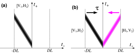
FIG. 2.: (a) Biphoton wave-function with femtosecond pulse pump in the case of Fig.1(a) shown in density plot. It differs significantly from the case of cw pumped type-II SPDC. It starts at $-DL$ and ends at $0$ due to the fact that a BBO is a negative uniaxial crystal so that the group velocity of the e-polarization is greater than that of the o-polarization. This figure shows how the two-photon amplitude $|V_{1},H_{2}\rangle$ is distributed in time. (b) Two biphoton amplitudes ($|V_{1},H_{2}\rangle$ and $|H_{1},V_{2}\rangle$) are present in the case of the experimental setup shown in Fig.1(b). When $\tau$ is increased, the two biphoton wave-functions move toward each other. If the pump is cw, the biphoton is essentially infinitely long in $t_{+}$ direction. If $\tau=DL/2$, in this case, the overlap is complete and 100% quantum interference can be observed. However, there is only limited amount of overlap due to the peculiar shape of the biphoton amplitudes in pulse pumped type-II SPDC and this results in the reduction of the visibility of quantum interference. This is the inherent difference from cw pumped type-II SPDC.

The shape of $\Pi(t_{+},t_{-})$ function is shown in Fig.2(a). It differs from the cw pumped type-II SPDC significantly. Similar to the cw case, the biphoton starts at $t_{-}=0$ and ends at $|t_{-}|=DL$ [30], but unlike the cw case, there is a strong dependence on $t_{+}$ direction. This is the reason why quantum interference visibility is reduced in femtosecond pulse pumped type-II SPDC.

To prepare a polarization entangled state using type-II collinear SPDC, one first has to replace the polarization beam splitter ($PBS$) in Fig.1(a) with a non-polarizing 50/50 beam splitter ($NPBS$), see Fig.1(b), so that there are two biphoton amplitudes to contribute to a coincidence count: (i) the signal is transmitted and the idler is reflected at the $NPBS$ ($t-r$ or $|V_{1},H_{2}\rangle$ amplitude), or (ii) the signal is reflected and the idler is transmitted at the $NPBS$ ($r-t$ or $|H_{1},V_{2}\rangle$ amplitude). Here we only considered the coincidence contributing amplitudes: amplitude post-selection. When these two $t-r$ ($|V_{1},H_{2}\rangle$) and $r-t$ ($|H_{1},V_{2}\rangle$) amplitudes are made indistinguishable, a Bell state is prepared (modulo amplitude post-selection) and it can be confirmed experimentally by observing 100% quantum interference [18]. To make the two amplitudes indistinguishable, the e-o delay $\tau$ should be correctly chosen. A typical method to find the correct e-o delay $\tau$ is to observe Hong-Ou-Mandel dip when the e-o delay $\tau$ in Fig.1(b) is varied. One then fixes $\tau$ where the complete destructive (when analyzers are set at $A_{1}=A_{2}=45^{\circ}$) or constructive (when analyzers are set at $A_{1}=45^{\circ}$ and $A_{2}=-45^{\circ}$) interference occurs.

What happens in the experimental setup shown in Fig.1(b) can be understood easily in the biphoton picture shown in Fig.2(b). As discussed above, there are two biphoton amplitudes distributed in ($t_{+}$,$t_{-}$) space. The one on the left represents $|V_{1},H_{2}\rangle$ and the one on the right represents $|H_{1},V_{2}\rangle$. When the e-o delay $\tau=0$, there is no overlap, i.e, no quantum interference. As $\tau$ increases, the biphoton wave-functions move toward each other by $\tau$. In cw pumped type-II SPDC, when $\tau=DL/2$, the overlap between two amplitudes is complete since the biphoton amplitude is essentially independent of $t_{+}$, i.e., 100% quantum interference can be observed. On the other hand, in femtosecond pulse pumped type-II SPDC, as shown in Fig.2(b), the amount of overlap is very small even at $\tau=DL/2$. Due to the tilted shape of the biphoton amplitude, there can never be 100% overlap between the two amplitudes and this results in the reduction of the visibility of quantum interference. It is important to note that, by introducing $\tau$, we are shifting the biphoton amplitudes in $t_{-}$ direction only.

There are several ways to increase the overlap between the two biphoton amplitudes: (i) One can use a thin BBO crystal. In this case the relative area of overlap between the two biphoton amplitudes is increased (since $|DL|$ is decreased) by sacrificing the amount of photon flux. (ii) One can use very narrowband spectral filters in front of the detectors. In this case, the biphoton amplitudes get broadened strongly in $t_{-}$ direction, which results in increased overlap between the two amplitudes (The effect of spectral filtering in $t_{+}$ direction is much smaller than that in $t_{-}$ direction) [32]. Again, the available photon flux is reduced.

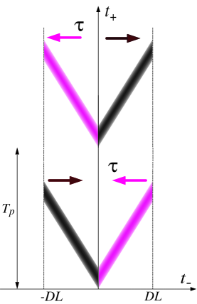
FIG. 3.: Biphoton amplitudes for Branning et al’s scheme. Four amplitudes are involved in the quantum interference, two from the first pass of the pump pulse (upper diagram) and two from the second pass of the pump pulse (lower diagram). The delay between the amplitudes from the first-pass and the second-pass is $T_{p}$. $\tau$ is the same e-o delay shown in Fig.1(b). The direction of arrows represent how the relevant amplitudes moves in $t_{-}$ direction when $\tau$ is increased.

Branning et al recently introduced an interferometric technique to overcome this problem by placing a type-II BBO crystal in a Michelson interferometer [26]. Such a method can in principle give a 100% quantum interference. It, however, cannot be used to prepare a polarization Bell state since there are four biphoton amplitudes, rather than two, involved in the interfering process [27]. In addition, the first-order interference (observed in single counting rates) cannot be avoided in Branning et al’s scheme [33]. Let us discuss this a little further. By placing a thick (5mm) type-II BBO crystal into a Michelson interferometer, Branning et al achieve a double-pass down-conversion scheme [34]. In this case, there are four biphoton amplitudes involved in the process: two from the first-pass of the pump pulse and the other two from the second-pass of the pump pulse since each pass of the pump pulse results in two biphoton amplitudes as shown in Fig.2(b). Then the non-zero contribution of the biphoton amplitudes in Branning et al’s scheme can be depicted as in Fig.3. $T_{p}$ is the delay introduced between the first-pass and the second-pass of the pump pulse, i.e. the delay between the two biphoton amplitudes from the first-pass of the pump pulse and the two biphoton amplitudes from the second-pass of the pump pulse. This delay $T_{p}$ is only introduced in $t_{+}$ direction. The e-o delay $\tau$ is introduced in $t_{-}$ direction by introducing a stack of quartz plates as before, see Fig.1(b) and Fig.2(b). When $\tau=0$ and $T_{p}=0$, 100% quantum interference should be observed if polarization information is erased by setting both analyzers at $45^{\circ}$. However, Bell states of the type shown in Eq.(2) have not been prepared in this method.

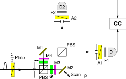
FIG. 4.: Bell state preparation scheme using two type-II BBO in a Mach-Zehnder interferometer. $T_{p}$ is the delay between the biphoton amplitudes from two different crystals. Therefore, the relative phase between the two amplitudes, $\varphi=\Omega_{p}T_{p}$. Note that the optic axes of the BBO crystals are oriented orthogonally, one vertically ($\updownarrow$) and the other horizontally ($\odot$). This is important with femtosecond pump pulse, but with cw pump it is of no importance. See text for detail.

Let us now consider the experimental setup shown in Fig.4 [37]. A type-II BBO crystal is placed in each arm of the Mach-Zehnder interferometer (MZI). The pump pulse is polarized at $45^{\circ}$ by using a $\lambda/2$ plate. PBS is the polarizing beam splitter. The optic axis of the first BBO is oriented vertically ($\updownarrow$) and the other horizontally ($\odot$). The pump pulse is blocked by the mirrors $M_{3}$ and $M_{4}$. There are only two biphoton amplitudes in this process, one from each crystal, due to the fact that a polarizing beam splitter is used to split the signal and the idler of the entangled photon pairs. Therefore, the quantum state, when the MZI is properly aligned, can be written as

$$|\psi\rangle=|H_{1},V_{2}\rangle+e^{i\varphi}|V_{1},H_{2}\rangle,$$ (15)

where $H$ and $V$ represent horizontal and vertical polarization respectively. Therefore, by varying the relative phase delay $\varphi$, one can prepare the Bell states $|\Psi^{\pm}\rangle$. The other two Bell states $|\Phi^{\pm}\rangle$ can be easily achieved by inserting a $\lambda/2$ plate in one output port of the MZI. Note that $\varphi=\Omega_{p}T_{p}$, where $T_{p}$ is the time delay between the two amplitudes in Eq.(15), so that by varying $T_{p}$, modulation in the coincidence counting rate is observed at the pump central frequency. Therefore, in this scheme, a true Bell state can be prepared without any post-selection methods. As we shall show later in this section, the thickness of the nonlinear crystals and the spectral filtering of the entangled photon flux do not affect the visibility in principle, even with a femtosecond pulse pump.

In this configuration, e-polarized photons are always detected by $D_{2}$ and o-polarized photons are always detected by $D_{1}$. This is of great importance when femtosecond laser is used as a pump. The biphoton amplitude for each coincidence detection event is shown in Fig.5. Note that only two biphoton amplitudes are involved in the quantum interference. If the MZI is balanced, 100% quantum interference can be observed. This provides a good method of preparing Bell states. If cw pump is used instead [38], it is not absolutely necessary to have the optic axes of the crystals orthogonally oriented. Suppose that the optic axis of the crystal in Fig.5(b) is now oriented vertically ($\updownarrow$), then the corresponding biphoton amplitude will appear flipped about $t_{-}=0$, thus appearing from 0 to $DL$. Clearly, there cannot be any overlap between two amplitudes even with the balanced MZI ($T_{p}=0$), just as the case considered in Fig.1(b) and Fig.2(b). However, in cw pump case, the biphoton amplitudes are independent of $t_{+}$. Therefore, by making appropriate compensation in $t_{-}$ direction, the two amplitudes can be overlapped: i.e., by setting the e-o delay $\tau=DL/2$. Note that if the coherence length of the cw pump laser is not long enough, then perfect overlap cannot be obtained for the same reason as in femtosecond pulse pumped case.

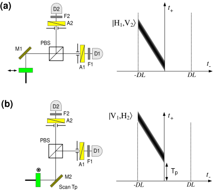
FIG. 5.: This figure illustrates the two interfering biphoton amplitudes in the experimental setup shown in Fig.4. $T_{p}$ is the time delay between the two biphoton amplitudes. If the MZI is balanced, i.e., $T_{p}=0$, complete overlap can be achieved.

So far, we have pictorially shown that a true Bell state can be obtained in femtosecond pulse pumped type-II SPDC by using an interferometric technique. The picture we have presented is based on the biphoton amplitude calculated earlier in this section. The space-time and polarization interference effects are calculated as follows. We use the right-hand coordinate system assuming the direction of propagation as $z$-axis. Then the sum of biphoton amplitudes in the experimental scheme Fig.4 is,

$${\mathcal{A}}(t_{+},T_{p},t_{-})=(\hat{e}_{1}\cdot\hat{e}_{H})(\hat{e}_{2}\cdot\hat{e}_{V})e^{-i\Omega_{p}t_{+}}\Pi(t_{+},t_{-})+$$ (16)

$$(\hat{e}_{1}\cdot\hat{e}_{V})(\hat{e}_{2}\cdot\hat{e}_{H})e^{-i\Omega_{p}(t_{+}+T_{p})}\Pi(t_{+}+T_{p},t_{-}),$$ (17)

where $\hat{e}$ represents the unit vector in a certain direction, for example, $\hat{e}_{1}$ represents the direction of the analyzer $A_{1}$. The coincidence counting rate is then calculated as

$$R_{c} = \int dt_{+}dt_{-}|{\mathcal{A}}(t_{+},T_{p},t_{-})|^{2}$$ (18)

$$= \int dt_{+}dt_{-}|\sin\theta_{1}\cos\theta_{2}\Pi(t_{+},t_{-})+$$ (20)

$$\hskip 50.58878pt\cos\theta_{1}\sin\theta_{2}e^{-i\Omega_{p}T_{p}}\Pi(t_{+}+T_{p},t_{-})|^{2}$$

$$\propto \sin^{2}\theta_{1}\cos^{2}\theta_{2}+\cos^{2}\theta_{1}\sin^{2}\theta_{2}+$$ (22)

$$2V(T_{p})\cos(\Omega_{p}T_{p})\sin\theta_{1}\cos\theta_{2}\cos\theta_{1}\sin\theta_{2},$$

where

$$V(T_{p}) \equiv \frac{\int dt_{+}dt_{-}\Pi(t_{+},t_{-})\Pi(t_{+}+T_{p},t_{-})}{\int dt_{+}dt_{-}\Pi^{2}(t_{+},t_{-})}$$ (23)

$$= e^{-[\sigma_{p}T_{p}]^{2}/8}.$$ (24)

Therefore, the space-time interference at $\theta_{1}=\theta_{2}=45^{\circ}$ will show

$$R_{c}=1+V(T_{p})\cos(\Omega_{p}T_{p}),$$ (25)

and the polarization interference will show

$$R_{c}=\sin^{2}(\theta_{1}+\theta_{2})\hskip 14.22636pt{\rm for}\hskip 14.22636pt\Omega_{p}T_{p}=0.$$ (26)

It is important to note that the envelope of the space-time interference when no spectral filters are used, $V(T_{p})$ function, is exactly equal to that of the self-convolution of the pump pulse. No crystal parameters affect the envelope of the space-time interference pattern. As we shall show in section IV, this is a special feature of type-II SPDC. If any spectral filtering is used, naturally, the envelope will be broadened.

III Bell state preparation using type-II SPDC: Experiment

As mentioned before, the goal of this section is to experimentally demonstrate that high-visibility quantum interference, which can be used to prepare a two-photon polarization Bell state, can be observed in the experimental scheme shown in Fig.4 and the envelope of this interference fringes is exactly the same as the pump pulse envelope.

Let us first discuss the experimental setup, see Fig.4. As briefly discussed in section II, a type-II BBO crystal is placed in each arm of the MZI and the optic axes of the crystals are oriented orthogonally, one vertically ($\updownarrow$) and the other horizontally ($\odot$). The thickness of the crystals is 3.4mm each. The crystals are pumped by frequency-doubled (by using a 700 $\mu$m type-I BBO) radiation of Ti:Sa laser oscillating at 90MHz. The pump has the central wavelength of 400nm. The average power of the laser beam in each arm of the MZI is approximately 10mW. The residual pump laser beam is blocked by two mirrors $M_{3}$ and $M_{4}$ and the relative phase $\varphi=\Omega_{p}T_{p}$ between the two amplitudes can be varied by adjusting one of the mirrors $M_{2}$. Collinear degenerate down-conversion is selected by a set of pinholes.

We first measure the envelope of the pump pulse itself by blocking the SPDC photons while detecting a small fraction of the pump light that passed through the mirrors $M_{3}$ and $M_{4}$. This is done by simply using another set of interference filters that transmit 400nm radiation. Fig.6 shows the measured envelope of the pump pulse interference patters. The measured FWHM is 170fsec and this will be compared with the envelope of the two-photon quantum interference patterns.

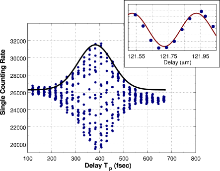
FIG. 6.: Observed pump pulse interference by blocking the SPDC photons. Solid line is a Gaussian fit to the envelope. The FWHM of the pump pulse envelope measured from the Gaussian fit is 170fsec. Each column of data represents the modulation of about one wavelength and the modulation period is 400nm as shown in the inset. The inset has the same vertical scale as the main figure and the delay is displayed in $\mu$m (rather than in fsec) to clearly show the modulation period. The inset shows the detailed modulation around $T_{p}\approx$ 406 fsec.

The space-time quantum interference is observed at $\theta_{1}=\theta_{2}=45^{\circ}$ by varying $T_{p}$. Two sets of experimental data are collected by using two different sets of interference filters, FWHM bandwidths of 10nm and 40nm with 800nm central wavelength, to demonstrate the effect of spectral filtering on the biphoton wave-function. 3nsec coincidence window is used and single counting rates of the detectors are recorded as well.

Fig.7 shows the data for these two measurements. In Fig.7(a), the FWHM of the interference envelope is 310 fsec. This shows that 10nm filter has some effect on the shape of the biphoton wave-function. This is not so surprising since the FWHM bandwidth of the SPDC spectrum for 3.4mm BBO is 3nm. However, when 40nm filters are used, see Fig.7(b), the FWHM of the envelope (170 fsec) is equal to the FWHM of the pump pulse interference patterns, see Fig.6. The effects of the spectral filters are not present and Eq.(25) is confirmed experimentally. The average visibility is 76% which is higher than in any femtosecond-pulse pumped type-II SPDC experiments with a thick crystal and no spectral filters. No interference is observed in the single detector counting rates.

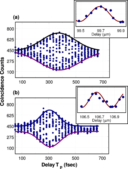
FIG. 7.: Quantum interference observed with the experimental setup shown in Fig.4. (a) 10nm filters are used. Accumulation time is 60sec. The measured width of the envelope is approximately 310 fsec. The visibility is $\approx$ 75%. (b) 40nm filters are used. Accumulation time is 80sec. The measured FWHM of the envelope is $\approx$ 170fsec which is equal to the FWHM envelope of the pump pulse itself. The visibility is $\approx$ 76%. Each column of data represent the modulation of about one wavelength with modulation period of 400nm as predicted in Eq.(25). The insets have the same vertical scales as the main figures and they show the detailed modulations around (a) $T_{p}\approx$ 332 fsec and (b) $T_{p}\approx$ 356 fsec.

The visibility loss is mostly due to the imperfect alignment of the system. Due to the anisotropy of the BBO crystal, e-ray walks off from the beam path of o-ray. Although both e-rays from the two different crystals are collected at the same detector, the walk-off is in different directions: one walks off horizontally, the other walks off vertically. When thick crystals are used, 3.4mm in our case, such effect is not negligible [39]. Since we are not interested in making any filtering, spectral or spatial, spatial filtering using a single mode fiber is not desirable. Instead of using spatial filtering, such a walk-off can be removed in another way: the two crystals are oriented in the same direction and then insert a $\lambda/2$ plate after one of the crystals [38].

The interferometry using the MZI, however, has one disadvantage: keeping the phase coherence between the two arms of the interferometer over a long time can be difficult. Although we have shown here that the visibility can be improved and in principle reach 100%, if the phase coherence is not kept for a long time, such a method is not useful as a source of Bell states for other experiments. We now turn our attention to type-I SPDC and investigate whether it offers a good solution to this problem. As we shall show, type-I SPDC offers a better way of preparing Bell states in femtosecond pulse pumped SPDC.

IV Bell state preparation using type-I SPDC: Theory

In this section, we discuss how one can prepare a polarization Bell state in an interferometric way using degenerate type-I SPDC pumped by a femtosecond pulse pump.

In general, the difference between type-II SPDC and type-I SPDC stems from calculating the phase mismatch term $\Delta$ in Eq.(7). In type-II SPDC, due to the fact that the signal and the idler photons have orthogonal polarization, only the first-order Taylor expansion of $\Delta$ is necessary, even in degenerate case. In degenerate type-I SPDC, however, one has to go to the second-order expansion since the first-order terms cancel if the frequencies are degenerate. Therefore, non-degenerate type-I SPDC formalism is basically the same as that of degenerate type-II SPDC and we will not discuss it here again. On the other hand, as we shall show, degenerate type-I SPDC differs quite a lot from type-II SPDC or non-degenerate type-I SPDC.

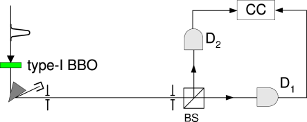
FIG. 8.: Most simple two-photon correlation experiment using type-I SPDC. See text for detail.

Let us first consider the experimental situation shown in Fig.8. Type-I SPDC occurs in the crystal and the photon pairs are detected by two detectors $D_{1}$ and $D_{2}$. The state of type-I SPDC is the same as Eq.(7) except that both photons are now $o$-polarized. For type-I degenerate SPDC, the phase mismatch term $\Delta$ becomes

$$\Delta=-\left(\nu_{p}D_{+}+\frac{1}{4}\nu_{-}^{2}D^{\prime\prime}\right),$$ (27)

where $\nu_{-}=\nu_{i}-\nu_{s}$ and subscripts $p$, $i$, and $s$ refer to the pump, idler, and the signal, respectively. $D_{+}=1/u_{o}(\Omega_{p}/2)-1/u_{p}(\Omega_{p})$ where $u_{o}$ ($u_{p}$) are the group velocities of the $o$-polarized photon (the pump photon) inside the crystal and $D^{{}^{\prime\prime}}=d^{2}K_{o}/d\Omega^{2}|_{\Omega=\Omega_{p}/2}$ where the wavevector $K_{o}=\Omega n_{o}(\Omega)/c$. $n_{o}(\Omega)$ is the index of refraction of the crystal for a given frequency $\Omega$. Note that $D_{+}$ is defined differently from the type-II SPDC case.

Therefore, the biphoton amplitude $A(t_{+},t_{-})$ for type-I SPDC now becomes [23]

$$A(t_{+},t_{-}) = e^{-i\Omega_{p}t_{+}}\int_{-\infty}^{\infty}d\nu_{p}\int_{-\infty}^{\infty}d\nu_{-}\int_{0}^{L}dz$$ (28)

$$\times e^{-[\nu_{p}/\sigma_{p}]^{2}}e^{-i\left[\nu_{p}D_{+}+\nu_{-}^{2}D^{\prime\prime}/4\right]z}$$ (29)

$$\times e^{-i\nu_{p}t_{+}}e^{-i[\nu_{-}/2]t_{-}},$$ (30)

$$\equiv e^{-i\Omega_{p}t_{+}}\Pi(t_{+},t_{-}),$$ (31)

where

$$\Pi(t_{+},t_{-})=\int_{0}^{L}dz\frac{1}{\sqrt{z}}e^{-\sigma_{p}^{2}[t_{+}+D_{+}z]^{2}/4}e^{it_{-}^{2}/[4D^{{}^{\prime\prime}}z]}.$$ (32)

Unlike the pulse pumped type-II SPDC, the $\Pi(t_{+},t_{-})$ function is symmetric in $t_{-}$. To simplify the calculation, no spectral filters are assumed.

FIG. 9.: Experimental scheme for two type-I crystal. Now, a type-I BBO crystal is placed in each arm of the MZI and the optic axes are orthogonally oriented. The output beam splitter (NPBS) of the MZI is now 50/50 non-polarizing beam splitter.

Having calculated the effective biphoton wave-function of type-I SPDC, let us now consider the experimental scheme shown in Fig.9 and calculate the coincidence counting rate in detail. Two interfering amplitudes are created from the two crystals similar to Fig.5 except that the biphoton amplitudes now look different in type-I SPDC. In the single-mode approximation, the quantum state prepared in the experimental setup of Fig.9 is given by

$$|\psi\rangle=|V_{1},V_{2}\rangle+e^{i\varphi}|H_{1},H_{2}\rangle,$$ (33)

where $\varphi$ is the relative phase similar to Eq.(33). When the phase $\varphi$ is correctly chosen, the Bell states $|\Phi^{\pm}\rangle$ can be prepared. (Note also that by inserting a $\lambda/2$ plate in one output port of the NPBS, the other two Bell states $|\Psi^{\pm}\rangle$ can also be prepared.) As we shall show below, there is no need for any spectral post-selection in this case, however, amplitude post-selection is assumed because there are possibilities that the signal and the idler exit at the same output port of the beamsplitter. This event, however, is not detected since we only consider the coincidence contributing events. Such amplitude post-selection is not desirable in principle. Luckily, there is a way to get around this problem which we shall briefly discuss in section V.

Let us now calculate the coincidence counting rates for the experimental setup shown in Fig.9 using the biphoton amplitude calculated in Eq.(31). By using the right-hand coordinate system as in type-II SPDC case, the coincidence counting rate is given by

$$R_{c} \propto \int dt_{+}dt_{-}|-\sin\theta_{1}\sin\theta_{2}\Pi(t_{+},t_{-})+$$ (35)

$$\hskip 50.58878pt\cos\theta_{1}\cos\theta_{2}e^{-i\Omega_{p}T_{p}}\Pi(t_{+}+T_{p},t_{-})|^{2}$$

$$= \sin^{2}\theta_{1}\sin^{2}\theta_{2}+\cos^{2}\theta_{1}\cos^{2}\theta_{2}-$$ (37)

$$2G(T_{p})\cos(\Omega_{p}T_{p})\sin\theta_{1}\sin\theta_{2}\cos\theta_{1}\cos\theta_{2},$$

where $G(t)=g(t)/g(0)$ with

$$g(t)=\int dt_{+}dt_{-}\Pi(t_{+},t_{-})\Pi^{*}(t_{+}+t,t_{-}).$$

The $G(t)$ function gives the envelope of the quantum interference pattern as a function of $t$.

Therefore, the space-time interference at $\theta_{1}=\theta_{2}=45^{\circ}$ will show

$$R_{c}=1-G(T_{p})\cos(\Omega_{p}T_{p}),$$ (38)

and the polarization interference will show

$$R_{c}=\cos^{2}(\theta_{1}+\theta_{2})\hskip 14.22636pt{\rm for}\hskip 14.22636pt\Omega_{p}T_{p}=0.$$ (39)

The envelope function of type-I SPDC, $G(T_{p})$, differs a lot from that of the type-II SPDC, $V(T_{p})$. $g(T_{p})$ is calculated to be

$$g(T_{p}) = \int_{-\infty}^{\infty}dt_{+}\int_{-\infty}^{\infty}dt_{-}\Pi(t_{+},t_{-})\Pi^{*}(t_{+}+T_{p},t_{-})$$ (40)

$$= \int_{0}^{1}du_{1}\int_{0}^{1}du_{2}\int_{-\infty}^{\infty}dt_{+}\int_{-\infty}^{\infty}dt_{-}$$ (41)

$$\times e^{-\sigma_{p}^{2}[t_{+}+D_{+}Lu_{1}^{2}]^{2}/4}e^{it_{-}^{2}/[4D^{\prime\prime}Lu_{1}^{2}]}$$ (42)

$$\times e^{-\sigma_{p}^{2}[t_{+}+T_{p}+D_{+}Lu_{2}^{2}]^{2}/4}e^{-it_{-}^{2}/[4D^{\prime\prime}Lu_{2}^{2}]}$$ (43)

$$= C\int_{0}^{1}du_{1}\int_{0}^{1}du_{2}\frac{u_{1}u_{2}}{\sqrt{|u_{1}^{2}-u_{2}^{2}|}}$$ (44)

$$\times e^{-\sigma_{p}^{2}\{D_{+}L[u_{1}^{2}-u_{2}^{2}]-T_{p}\}^{2}/8},$$ (45)

where $C$ is a constant and the change of variable, $z_{i}=u_{i}^{2}L$ ($i=1,2$), has been made.

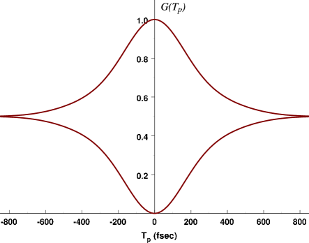
FIG. 10.: Calculated envelope of the interference pattern $G(T_{p})$ from Eq.(45) for the experimental parameters in our experiment. Note that there are long tails of the interference envelope.

It is interesting to find that the envelope function $G(T_{p})$ does not explicitly contain the second-order expansion of the phase mismatch term $D^{\prime\prime}$ at all. This result is quite surprising since the presence of $D^{\prime\prime}$ is the principal difference between type-II SPDC and degenerate type-I SPDC. (This is due to the fact that $D=0$ for degenerate type-I SPDC.) Note also that the envelope of the space-time interference is not simply that of the convolution of the pump pulse as in type-II SPDC shown in Eq.(25): it is a complicated function of $D_{+}L$ and $\sigma_{p}$. Fig.10 shows $G(T_{p})$ when realistic experimental parameters are substituted in Eq.(45).

V Bell state preparation using type-I SPDC: Experiment

In the experiment, we use two pieces of type-I BBO crystal cut for collinear degenerate SPDC. The thickness of the crystals is 3.4 mm each. The pump pulse central wavelength is 400nm and the average power of the pump beam in each arm of the MZI is approximately 10mW as in the type-II experiment. The repetition rate of the pump pulse is approximately 82MHz.

We first measured the pump pulse envelope. The BBO crystals are not removed from the MZI for the pump pulse envelope measurement. This data is shown in Fig.11. Gaussian fitting of the data gives the FWHM equal to 200 fsec. This is to be compared with the envelope of the quantum interference pattern measured in coincidence counting rate between the two detectors $D_{1}$ and $D_{2}$.

To observe the quantum interference, we first block all the residual pump radiation using additional absorption filters. Analyzer angles are set at $\theta_{1}=\theta_{2}=45^{\circ}$. The interference filters used in this measurement have 10nm bandwidth. As expected, high-visibility quantum interference is observed, see Fig.12. The FWHM of the interference envelope is much bigger than that of the pump pulse itself, see Fig.11. Unfortunately, due to rather large fluctuations in the data, long tails of the interference envelope predicted by Eq.(45), see Fig.10 are washed out.

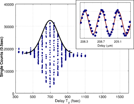
FIG. 11.: Pump pulse interference. The measured FWHM envelope is approximately 200fsec. Solid line is the Gaussian fit to the envelope. Each column of data represents the modulation of several wavelengths with modulation period of 400nm as shown in the inset. The inset has the same vertical scale as the main figure and it shows the detailed modulation around $T_{p}\approx$ 696 fsec.

With 40nm filters, the shape of the envelope remained almost the same, while the width of the envelope and the visibility is slightly reduced. The reduction of the visibility with 40nm filters is mainly due to the difficulty in aligning both crystals with broadband filters.

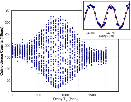
FIG. 12.: Space-time interference observed in coincidence between the two detectors $D_{1}$ and $D_{2}$ for the analyzer setting $\theta_{1}=\theta_{2}=45^{\circ}$. 10nm filters are used for this measurement. Note that the FWHM is much bigger than the pump pulse interference shown in Fig.11. 400nm modulation is observed as predicted in Eq.(38). The inset has the same vertical scale as the main figure and it shows the detailed modulation around $T_{p}\approx$ 826 fsec.

There are two problems with this method: (i) amplitude post-selection is assumed, and (ii) the MZI cannot be made very stable for a long term. In a recently published paper [40], the second problem was solved by using the “collinear interferometer” method in which two type-I crystals are placed collinearly with the optic axes orthogonally oriented. The first problem, amplitude post-selection, was also removed by employing non-degenerate type-I SPDC in the collinear scheme [41]. Also with collinear method, aligning the crystals is much easier and the visibility as high as 92% was easily obtained with 40nm filters [40]. Although the collinear method and the MZI method look different, the theoretical description we have presented in the previous sections applies with no modifications. The theory described in section IV explains all the experimental results of Ref.[40] in detail and the experimental results shown in Ref.[41] can be explained by using the theory described in section II by exchanging the polarization label with frequency label.

VI Conclusion

We have shown that high-visibility quantum interference can be observed without using narrow-band filters for both type-II and type-I SPDC pumped by femtosecond laser pulses. In these methods, a Mach-Zehnder interferometer is used to coherently add two biphoton amplitudes from two different nonlinear crystals pumped by coherent laser pulses. Using this method, maximally entangled two-photon polarization states, or Bell states, can be successfully prepared.

It is important to note that biphoton or two-photon amplitudes generated from coherent pump laser remain coherent even though they may originate from different spatial [35] or temporal [32, 36, 42] domains . As long as the distinguishing information present in the interfering amplitudes are erased, high-visibility quantum interference should be observed.

There is, however, one problem with the method using a Mach-Zehnder interferometer: keeping the phase coherence is difficult. This is a rather serious problem especially when one is interested in using such a method to prepare a Bell state and use it as a source. The collinear two-photon interferometer solves this problem. In this method, two type-I crystals are placed collinearly in the pump beam path [40, 41]. Although different geometry is used, the theory presented in section IV applies equally for both Mach-Zehnder interferometer and collinear case.

For the two-crystal scheme using pulse pumped type-II SPDC, the envelope of the space-time interference pattern is determined only by the bandwidth of the pump pulse $\sigma_{p}$, as shown in section II and section III. Crystal parameters do not affect the envelope of the interference pattern at all. On the other hand, for the two-crystal scheme using pulse pumped type-I SPDC, the envelope of the interference pattern strongly depends on the crystal parameters, especially on $D_{+}=1/u_{o}(\Omega_{p}/2)-1/u_{p}(\Omega_{p})$ and the crystal thickness $L$ as well as the pump bandwidth $\sigma_{p}$, as shown in section IV and section V. It is also interesting to note that the envelope of the interference pattern does not have explicit dependence on $D^{\prime\prime}$.

It is important to note the following. To observe the space-time interference, one can introduce the delay in two ways: (i) in $t_{-}$ or (ii) in $t_{+}$. In the single-crystal SPDC scheme, quantum interference is observed by introducing the delay $\tau$ in $t_{-}$. But in two-crystal SPDC scheme, one can introduce either in $t_{-}$ or in $t_{+}$. In this paper, we have demonstrated high-visibility quantum interference in femtosecond pulse pumped SPDC by introducing a delay $T_{p}$ in $t_{+}$.

In conclusion, we have demonstrated Bell states preparation schemes using femtosecond pulse pumped SPDC. In type-II SPDC, the envelope of the interference pattern is exactly equal to the envelope of the pump pulse convolution. On the other hand, the envelope of interference pattern from type-I SPDC is much broader than that of the pump interference. This may be useful if one needs to use femtosecond pulse pumped SPDC, yet requires that two-photon amplitudes are distributed in time more than the pump pulse itself. Type-I SPDC has an advantage over type-II SPDC: two crystals can be easily used collinearly. As demonstrated in [40, 41], such a method will serve as a good source of entangled photon pairs for experiments which require accurate timing to overlap biphotons from different domains.

REFERENCES

- [1] E. Schrödinger, Naturwissenschaften 23, 807 (1935); 23, 823 (1935); 23, 844 (1935); the English translation appears in Quantum Theory and Measurement, edited by J.A. Wheeler and W.H. Zurek (Princeton University Press, New York, 1983).
- [2] A. Einstein, B. Podolsky, and N. Rosen, Phys. Rev. 47, 777 (1935).
- [3] D. Bohm, Quantum Theory (Prentice-Hall Inc., New York, 1951).
- [4] J.S. Bell, Speakable and unspeakable in quantum mechanics, (Cambridge University Press, New York, 1987).
- [5] S.J. Freedman and J.F. Clauser, Phys. Rev. Lett. 28, 938 (1972); J.F. Clauser and A. Shimony, Rep. Prog. Phys. 41, 1881 (1978).
- [6] A. Aspect, P. Grangier, and G. Roger, Phys. Rev. Lett. 47, 460 (1981); A. Aspect, J. Dalibard, and G. Roger, Phys. Rev. Lett. 49, 1804 (1982); A. Aspect, P. Grangier, G. Roger, Phys. Rev. Lett. 49, 91 (1982).
- [7] C.O. Alley and Y.H. Shih, Proc. of 2nd Int. Symp. Foundations of Quantum Mechanics, ed. M. Namiki (Physical Society of Japan, Tokyo) (1987); Y.H. Shih and C.O. Alley, Phys. Rev. Lett. 61, 2921 (1988).
- [8] J.G. Rarity and P.R. Tapster, Phys. Rev. Lett. 64, 2495 (1990); G. Weihs, T. Jennewein, C. Simon, H. Weinfurter, and A. Zeilinger, Phys. Rev. Lett. 81, 5039 (1998).
- [9] T. Jennewein, C. Simon, G. Weihs, H. Weinfurter, and A. Zeilinger, Phys. Rev. Lett. 84, 4729 (2000); D.S. Naik, C.G. Peterson, A.G. White, A.J. Berglund, and P.G. Kwiat, Phys. Rev. Lett. 84, 4733 (2000); W. Tittel, J. Brendel, H. Zbinden, and N. Gisin, Phys. Rev. Lett. 84, 4737 (2000).
- [10] C.H. Bennett, G. Brassard, C. Crépeau, R. Jozsa,A. Peres, and W.K. Wootters , Phys. Rev. Lett. 70, 1895 (1993); D. Bouwmeester, J.-W. Pan, M. Eibl, H. Weinfurter, and A. Zeilinger , Nature 390, 575 (1997); D. Boschi, S. Branca, F. De Martini, L. Hardy, and S. Popescu, Phys. Rev. Lett. 80, 1121 (1998); A. Furusawa, J.L. Srensen, S.L. Braunstein, C.A. Fuchs, H.J. Kimble, E.S. Polzik, Science 282, 706 (1998); Y.-H. Kim, S.P. Kulik, and Y.H. Shih, Phys. Rev. Lett. 86, 1370 (2001).
- [11] D.N. Klyshko, Photons and Nonlinear Optics, (Gordon and Breach, 1988).
- [12] D.N. Klyshko, Soviet Phys-JETP Lett. 6, 23 (1967).
- [13] Ya. B. Zel’dovich and D.N. Klyshko, JETP Lett. 9, 40 (1969).
- [14] D.C. Burnham and D.L. Weinberg, Phys. Rev. Lett. 25, 84 (1970).
- [15] D.N. Klyshko, Sov. J. Quantum Electron. 7, 591 (1977); M.F. Vlasenko, G. Kh. Kitaeva, and A.N. Penin, Sov. J. Quantum Electron. 10, 252 (1980).
- [16] D.N. Klyshko, Sov. J. Quantum Electron. 10, 1112 (1980); A.A. Malygin, A.N. Penin, and A.V. Sergienko, JETP Lett. 33, 477 (1981); J.G. Rarity, K.D. Ridley, and P.R. Tapster, Applied Optics 26, 4616 (1987).
- [17] C.K. Hong, Z.Y. Ou, and L. Mandel, Phys. Rev. Lett. 59, 2044 (1987).
- [18] Y.H. Shih and A.V. Sergienko, Phys. Lett. A 186, 29 (1994); Phys. Lett. A 191, 201 (1994).
- [19] L. De Caro and A. Garuccio, Phys. Rev. A 50, R2803 (1994).
- [20] P.G. Kwiat, K. Mattle, H. Weinfurter, A. Zeilinger, A.V. Sergienko, and Y.H. Shih, Phys. Rev. Lett. 75, 4337 (1995);
- [21] P.G. Kwiat, E. Waks, A.G. White, I. Appelbaum, and P.H. Eberhard, Phys. Rev. A 60, R773 (1999).
- [22] A.V. Burlakov, M.V. Chekhova, O.A. Karabutova, D.N. Klyshko, and S.P. Kulik, Phys. Rev. A 60, R4209 (1999); A.V. Burlakov and D.N. Klyshko, JETP Lett. 69, 839 (1999).
- [23] T.E. Keller and M.H. Rubin, Phys. Rev. A 56, 1534 (1997).
- [24] A.V. Sergienko, M. Atatüre, Z. Walton, G. Jaeger, B.E.A. Saleh, and M.C. Teich, Phys. Rev. A 60, R2622 (1999).
- [25] W.P. Grice and I.A. Walmsley, Phys. Rev. A 56, 1627 (1997); G. Di Giuseppe, L. Haiberger, F. De Martini, A.V. Sergienko, Phys. Rev. A 56, R21 (1997); W.P. Grice, R. Erdmann, I.A. Walmsley, D. Branning, Phys. Rev. A 57, R2289 (1998).
- [26] D. Branning, W.P. Grice, R. Erdmann, and I.A. Walmsley, Phys. Rev. Lett 83, 955 (1999); Phys. Rev. A 62, 013814 (2000).
- [27] It should be noted that Branning et al do not claim Bell state preparation in Ref.[26]. In this paper, we simply point out that the experimental scheme demonstrated in Ref.[26] cannot be used to prepare a Bell state which is of our interest.
- [28] M. Atatüre, A.V. Sergienko, B.E.A. Saleh, and M.C. Teich, Phys. Rev. Lett. 84, 618 (2000).
-
[29]
Y.-H. Kim, S.P. Kulik, M.H. Rubin, and Y.H. Shih,
quant-ph/0006003. - [30] M.H. Rubin, D.N. Klyshko, Y.H. Shih, and A.V. Sergienko , Phys. Rev. A 50, 5122 (1994).
- [31] R.J. Glauber, Phys. Rev. 130, 2529 (1963).
- [32] Y.-H. Kim, V. Berardi, M.V. Chekhova, A. Garuccio, and Y.H. Shih, Phys. Rev. A 62, 043820 (2000).
- [33] The presence of the first-order interference in Branning et al’s scheme is not surprising. Similar effects are already observed by many authors, see Ref.[32, 35, 36]. First-order interference, although very interesting, is not desirable here and there should not be any first-order interference the purpose of Bell state preparation.
- [34] Branning et al’s scheme uses a plate and a polarizing beam splitter. This setup is essentially equivalent to the scheme with polarizers set at . As pointed out in Ref.[27], Branning et al do not claim Bell state preparation and therefore there is no need for varying the angles of the analyzers. We are, however, focused on Bell state preparation. Therefore, it is necessary that angles of the analyzers can be varied arbitrarily.
- [35] X.Y. Zou, L.J. Wang, and L. Mandel, Phys. Rev. Lett. 67, 318 (1991); T.J. Herzog, J.G. Rarity, H. Weinfurter, and A. Zeilinger, Phys. Rev. Lett. 72, 629 (1994); A.V. Burlakov, M.V. Chekhova, D.N. Klyshko, S.P. Kulik, A.N. Penin, Y.H. Shih, and D.V. Strekalov, Phys. Rev. A 56, 3214 (1997).
- [36] Y.-H. Kim, M.V. Chekhova, S.P. Kulik, Y.H. Shih, and M.H. Rubin, Phys. Rev. A 61, 051803(R) (2000).
- [37] Kwiat et al proposed a similar scheme with cw pumped SPDC for the purpose of loophole-free test of Bell’s inequality, see Ref.[38].
- [38] P.G. Kwiat, P.H. Eberhard, A.M. Steinberg, and R.Y. Chiao, Phys. Rev. A 49, 3209 (1994).
- [39] For 3.4mm type-II phased matched (400/800nm) BBO crystal, the maximum transverse walk-off between the e-ray and the o-ray is m. Compared to 2.5mm beam diameter, this is not big, but certainly not negligible.
- [40] Y.-H. Kim, S.P. Kulik, and Y.H. Shih, Phys. Rev. A 62, 011802(R) (2000).
-
[41]
Y.-H. Kim, S.P. Kulik, and Y.H. Shih,
quant-ph/0007067. - [42] Y.-H. Kim, M.V. Chekhova, S.P. Kulik, and Y.H. Shih, Phys. Rev. A 60, R37 (1999).