Entanglement generation and degradation by passive optical devices

Abstract

The influence of losses in the interferometric generation and the transmission of continuous-variable entangled light is studied, with special emphasis on Gaussian states. Based on the theory of quantum-state transformation at absorbing dielectric devices, the amount of entanglement is quantified by means of the relative-entropy measure. Upper bounds of entanglement and the distance to the set of separable Gaussian states are calculated. Compared with the distance measure, the bounds can substantially overestimate the entanglement. In particular, they do not show the drastic decrease of entanglement with increasing mean photon number, as does the distance measure.

I Introduction

Entangled quantum states containing more than one photon on average have been of increasing interest (see for example [1]) for several reasons. So, maximally entangled continuous-variable states of EPR type require infinitely large mean numbers of photons. Another reason is that such states might be more robust against decoherence. If, for example, in an experiment with Bell states one photon is lost, e.g. absorbed, during the transmission from a sender to a receiver, the entanglement is immediately gone (the state is projected onto a separable state). States with more than one photon on average have the advantage that even a few photons might get lost on the way (leaving behind some mixed state), but inseparability might still be preserved, that is, maximally entangled photon pairs could still be extracted by means of purification procedures [2, 3, 4].

The aim of the present article is to investigate entanglement properties of bipartite quantum states that generically live in infinite-dimensional Hilbert spaces. Typical examples are Gaussian states such as two-mode squeezed vacuum states, which are the states commonly used in quantum communication of continuous-variable systems [5]. They are also the states we will be looking at in what follows.

In real experiments, both in quantum-state generation and processing, e.g., transmission through generically lossy optical systems such as fibers, the necessarily existing interaction of the light fields with dissipative environments spoils the quantum-state purity, leaving behind statistical mixtures. Unfortunately, quantification of entanglement for mixed states in infinite-dimensional Hilbert spaces is yet impossible in practice. It typically involves minimizations over infinitely many parameters, as it is the case for the entropy of formation as well as for the distance to the set of all separable quantum states measured either by the relative entropy or Bures’ metric [6]. It is, however, possible to derive upper bounds on the entanglement content [7] by using the convexity property of the relative entropy. For Gaussian states, however, we derive an upper bound based on the distance to the set of separable Gaussian states which is far better than the convexity bound. These bounds may be very useful for estimation of the entanglement degradation in real quantum information systems.

The article is organized as follows. In Section II the influence of losses in the interferometric entanglement generation at a beam splitter is studied. A typical situation in quantum communication is considered in Section III, in which the entanglement degradation of a two-mode squeezed vacuum (TMSV) state is transmitted through a noisy communication channel say, two lossy optical fibers, is examined. Some concluding remarks are given in Section IV.

II Entanglement generation by mixing squeezed vacua at a beam splitter

A Lossless beam splitters

Let us first consider the case of a lossless beam splitter and (quasi-)monochromatic light of (mid-)frequency $\omega$ (Fig. 1). It is well known [8, 9, 10, 11, 12, 13] that a lossless beam splitter transforms the operators of the incoming modes $\hat{a}_{1}(\omega)$ and $\hat{a}_{2}(\omega)$ to the operators of the outgoing modes $\hat{b}_{1}(\omega)$ and $\hat{b}_{2}(\omega)$ according to

$${\hat{b}_{1}(\omega)\choose\hat{b}_{2}(\omega)}={\bf T}(\omega){\hat{a}_{1}(\omega)\choose\hat{a}_{2}(\omega)},$$ (1)

where ${\bf T}(\omega)$ is the unitary characteristic transformation matrix of the beam splitter. Equivalently, the operators can be left unchanged and instead the density operator is transformed with the inverse matrix ${\bf T}^{-1}(\omega)$ $\!=$ $\!{\bf T}^{+}(\omega)$ according to

$$\hat{\varrho}_{\rm out}=\hat{\varrho}_{\rm in}\!\left[{\bf T}^{+}(\omega){\hat{a}_{1}(\omega)\choose\hat{a}_{2}(\omega)}\,,{\bf T}^{\rm T}(\omega){\hat{a}_{1}^{\dagger}(\omega)\choose\hat{a}_{2}^{\dagger}(\omega)}\right].$$ (2)

Let each of the two incoming modes be prepared in a squeezed vacuum state, i.e.,

$$\hat{\varrho}_{\rm in}=|\Psi_{\rm in}\rangle\langle\Psi_{\rm in}|$$ (3)

where

$$|\Psi_{\rm in}\rangle=\hat{S}_{1}\hat{S}_{2}|0,0\rangle,$$ (4)

with $\hat{S}_{i}$ ($i$ $\!=$ $\!1,2$) being the (single-mode) squeeze operator

$$\hat{S}_{i}=\exp\!\left[-\textstyle\frac{1}{2}\left(\xi_{i}\hat{a}_{i}^{\dagger 2}-\xi_{i}^{\ast}\hat{a}_{i}^{2}\right)\right]$$ (6)

$$\hskip 8.61108pt=\exp\!\left(-\textstyle\frac{1}{2}q_{i}\hat{a}_{i}^{\dagger 2}\right)\left(1\!-\!|q_{i}|^{2}\right)^{(2\hat{n}_{i}+1)/4}\exp\!\left(\textstyle\frac{1}{2}q_{i}^{\ast}\hat{a}_{i}^{2}\right)$$

($q_{i}$ $\!=$ $\!\tanh|\xi_{i}|e^{i\phi_{i}}$, $\phi_{i}$ $\!=$ $\!\arg\xi_{i}$). Here, the second line follows from general disentangling theorems [14, 15]. By Eq. (2), the output quantum state is

$$\hat{\varrho}_{\rm out}=|\Psi_{\rm out}\rangle\langle\Psi_{\rm out}|,$$ (7)

where

$$|\Psi_{\rm out}\rangle=\left[(1-|q_{1}|^{2})(1-|q_{2}|^{2})\right]^{1/4}$$ (10)

$$\hskip 17.22217pt\times\,\exp\!\left[-\textstyle\frac{1}{2}q_{1}\big{(}T_{11}\hat{a}_{1}^{\dagger}+T_{21}\hat{a}_{2}^{\dagger}\big{)}^{2}\right.$$

$$\hskip 25.83325pt\left.-\,\textstyle\frac{1}{2}q_{2}\big{(}T_{12}\hat{a}_{1}^{\dagger}+T_{22}\hat{a}_{2}^{\dagger}\big{)}^{2}\right]|0,0\rangle.$$

The $T_{ij}$ are the elements of the characteristic transformation matrix ${\bf T}$ (at chosen mid-frequency), which can be given, without loss of generality, in the form of

$${\bf T}=\left(\begin{array}[]{cc}T&R\\ -R^{\ast}&T^{\ast}\end{array}\right),$$ (11)

with $T$ $\!=$ $\!|T|{\rm e}^{i\phi_{T}}$ and $R$ $\!=$ $\!|R|{\rm e}^{i\phi_{R}}$ being the (complex) transmission and reflection coefficients of the beam splitter.

From inspection of Eq. (7) it is seen that the preparation of an entangled state is controlled by the parameter

$$\xi_{12}=q_{1}T_{11}T_{21}+q_{2}T_{12}T_{22}=-q_{1}TR^{\ast}+q_{2}RT^{\ast}.$$ (12)

When $\xi_{12}$ $\!=$ $\!0$ is valid, then the output state is separable. This is the case for $\phi_{1}$ $\!-$ $\!\phi_{2}$ $\!+$ $\!2(\phi_{T}$ $\!-$ $\!\phi_{R})$ $\!=$ $\!0$ and $|q_{1}|$ $\!=$ $\!|q_{2}|$. On the other hand, if again $|q_{1}|$ $\!=$ $\!|q_{2}|$ $\!=$ $\!|q|$ but $\phi_{1}$ $\!-$ $\!\phi_{2}$ $\!+2(\phi_{T}$ $\!-\phi_{R})$ $\!=$ $\!\pm\pi$, then for $|TR|$ $\!=$ $\!1/2$ the output quantum state is just a TMSV state,

$$|\Psi_{\rm out}\rangle=|{\rm TMSV}\rangle=\sqrt{1-|q|^{2}}\,\exp\!\left[-q\hat{a}_{1}^{\dagger}\hat{a}_{2}^{\dagger}\right]|0,0\rangle,$$ (13)

where

$$q=|q|^{i(\phi_{2}+\phi_{R}-\phi_{T})}=-|q|{\rm e}^{i(\phi_{1}+\phi_{T}-\phi_{R})}.$$ (14)

Since, according to Eq. (7), the output quantum state is a pure state, entanglement is uniquely measured by the von Neumann entropy of the (reduced) quantum state of either of the output modes,

$$E(\hat{\varrho}_{\rm out})=S_{1(2)}=-{\rm Tr}\bigl{[}\hat{\varrho}_{1(2)}\ln\hat{\varrho}_{1(2)}\bigr{]},$$ (15)

where $\hat{\varrho}_{1(2)}$ denotes the (reduced) output density operator of mode $1(2)$, which is obtained by tracing $\hat{\varrho}_{\rm out}$ with respect to mode $2(1)$. The result of the numerical calculation is illustrated in Figs. 2 and 3 for a $50\%/50\%$ beam splitter. In Fig. 2 the phases are chosen such that the relation $\phi_{1}$ $\!-$ $\!\phi_{2}$ $\!+2(\phi_{T}$ $\!-\phi_{R})$ $\!=$ $\!\pm\pi$ is valid, thus leading to a TMSV state for $|q_{1}|$ $\!=$ $\!|q_{2}|$. Figure 3 shows the case where $\phi_{1}$ $\!-$ $\!\phi_{2}$ $\!+2(\phi_{T}$ $\!-\phi_{R})$ $\!=$ $0$, so that for $|q_{1}|$ $\!=$ $\!|q_{2}|$ no entanglement is observed. Note that using squeezed coherent states instead of squeezed vacuum states does not change the entanglement. This is due to the fact that coherent shifts are unitary operations on subsystems which leave any entanglement measure invariant.

B Lossy beam splitters

In practice there are always some losses and things get slightly more complicated. The SU(2) group transformation in Eq. (1) has to be replaced by a SU(4) group transformation, where the unitary transformation acts in the product Hilbert space of the field modes and the device modes [16, 17, 18]. As a result, Eqs. (1) and (2), respectively, have to be replaced by

$$\hat{\mbox{\boldmath$\beta$}}(\omega)=\mbox{\boldmath$\Lambda$}(\omega)\,\hat{\mbox{\boldmath$\alpha$}}(\omega)$$ (16)

and

$$\hat{\varrho}_{\rm out}^{({\rm F})}={\rm Tr}^{({\rm D})}\hat{\varrho}_{\rm in}\!\left[\mbox{\boldmath$\Lambda$}^{+}(\omega)\hat{\mbox{\boldmath$\alpha$}}(\omega),\mbox{\boldmath$\Lambda$}^{\rm T}(\omega)\hat{\mbox{\boldmath$\alpha$}}^{\dagger}(\omega)\right],$$ (17)

where the “four-vector” notation $\hat{\mbox{\boldmath$\alpha$}}(\omega)$ for abbreviating the list of operators $\hat{a}_{1}(\omega)$, $\hat{a}_{2}(\omega)$, $\hat{g}_{1}(\omega)$, $\hat{g}_{2}(\omega)$ [and $\hat{\mbox{\boldmath$\beta$}}(\omega)$ accordingly] has been used. The SU(4) group element $\mbox{\boldmath$\Lambda$}(\omega)$ is expressed in terms of the characteristic transformation and absorption matrices ${\bf T}(\omega)$ and ${\bf A}(\omega)$ of the beam splitter as

$$\mbox{\boldmath$\Lambda$}(\omega)=\left(\!\begin{array}[]{cc}{\bf T}(\omega)&{\bf A}(\omega)\\[2.15277pt] -{\bf S}(\omega){\bf C}^{-1}(\omega){\bf T}(\omega)&{\bf C}(\omega){\bf S}^{-1}(\omega){\bf A}(\omega)\end{array}\!\right)$$ (18)

with the commuting positive Hermitian matrices

$${\bf C}(\omega)=\sqrt{{\bf T}(\omega){\bf T}^{+}(\omega)}\,,\quad{\bf S}(\omega)=\sqrt{{\bf A}(\omega){\bf A}^{+}(\omega)}\,.$$ (19)

From the above, the output density matrix in the Fock basis can be given in the form of (Appendix A):

$$\langle m_{1},m_{2}|\hat{\varrho}_{\rm out}^{({\rm F})}|n_{1},n_{2}\rangle$$ (22)

$$\hskip 8.61108pt=\sqrt{\frac{(1\!-\!|q_{1}|^{2})(1\!-\!|q_{2}|^{2})}{m_{1}!m_{2}!n_{1}!n_{2}!}}(-1)^{m_{1}+m_{2}+n_{1}+n_{2}}$$

$$\hskip 8.61108pt\times\sum\limits_{g_{1},g_{2}=0}^{\infty}\frac{1}{g_{1}!g_{2}!}{\rm H}^{\bf M}_{m_{1},m_{2},g_{1},g_{2}}({\bf 0}){\rm H}^{\ast{\bf M}}_{n_{1},n_{2},g_{1},g_{2}}({\bf 0}),$$

where ${\rm H}^{\bf M}_{n}({\bf 0})$ denotes the Hermite polynomial of four variables with zero argument, generated by the symmetric matrix ${\bf M}$ with elements

$$M_{ij}=q_{1}\Lambda_{i1}\Lambda_{j1}+q_{2}\Lambda_{i2}\Lambda_{j2}\,.$$ (23)

Note that in Eq. (22) it is assumed that the device is prepared in the ground state.

In order to quantify the entanglement content of a mixed state $\hat{\varrho}$, such as $\hat{\varrho}_{\rm out}^{({\rm F})}$ in Eq. (22), we make use of the relative entropy measuring the distance of the state to the set ${\cal S}$ of all separable states $\hat{\sigma}$ [6],

$$E(\hat{\varrho})=\min_{\hat{\sigma}\in{\cal S}}{\rm Tr}\big{[}\hat{\varrho}\big{(}\ln\hat{\varrho}-\ln\hat{\sigma}\big{)}\big{]}\,.$$ (24)

For pure states this measure reduces to the von Neumann entropy (15) of either of the subsystems which can be computed by means of Schmidt decomposition of the continuous-variable state [4]. It is also known that when the quantum state has the Schmidt form,

$$\hat{\varrho}=\sum\limits_{n,m}C_{n,m}|\phi_{n},\psi_{n}\rangle\langle\phi_{m},\psi_{m}|,$$ (25)

then the amount of entanglement measured by the relative entropy is given by [19, 20]

$$E(\hat{\varrho})=-\sum_{n}C_{n,n}\ln C_{n,n}-S(\hat{\varrho}).$$ (26)

Unfortunately, there is no closed solution of Eq. (24) for arbitrary mixed states. Nevertheless, upper bounds on the entanglement can be calculated [7], representing the quantum state under study in terms of states in Schmidt decomposition and using the convexity of the relative entropy,

$$E\Bigl{(}\sum_{n}p_{n}\hat{\varrho}_{n}\Bigr{)}\leq\sum_{n}p_{n}E(\hat{\varrho}_{n}),\quad\sum_{n}p_{n}=1.$$ (27)

Applying the method to the output quantum state in Eq. (22), i.e., rewriting it in the form of

$$\hat{\varrho}_{\rm out}^{({\rm F})} = \sum\limits_{k,l=0}^{\infty}C_{k,l,0}|k,k\rangle\langle l,l|$$ (30)

$$+\sum\limits_{m=1}^{\infty}\sum\limits_{k,l=0}^{\infty}C_{k,l,m}|k+m,k\rangle\langle l+m,l|$$

$$+\sum\limits_{m=1}^{\infty}\sum\limits_{k,l=0}^{\infty}C_{k,l,m}|k,k+m\rangle\langle l,l+m|$$

$$= p_{0}\hat{\varrho}_{0}+\sum\limits_{m=1}^{\infty}p_{m}\hat{\varrho}_{m,1}+\sum\limits_{m=1}^{\infty}p_{m}\hat{\varrho}_{m,2}\,,$$ (31)

the inequality (27) leads to

$$E\big{(}\hat{\varrho}_{\rm out}^{({\rm F})}\big{)}\leq p_{0}E(\hat{\varrho}_{0})+\sum\limits_{m=1}^{\infty}p_{m}\left[E(\hat{\varrho}_{m,1})+E(\hat{\varrho}_{m,2})\right],$$ (32)

where $E(\hat{\varrho}_{0})$, $E(\hat{\varrho}_{m,1})$, and $E(\hat{\varrho}_{m,2})$ can be determined according to Eq. (26). In the numerical calculation we have used the dielectric-plate model of a beam splitter, taking the ${\bf T}$ and ${\bf A}$ matrices from [18, 21]. The result is illustrated in Fig. 4, which shows the dependence on the plate thickness of the upper bound of the attainable entanglement. The oscillations are due to phase matching and phase mismatch at certain beam splitter thicknesses [cf. Eq. (12)]. Note that the local minima of the curve for the lossy beam splitter never go down to zero as do the corresponding minima of the curve for the lossless beam splitter. This obviously reflects the fact that the result for the lossless beam splitter is exact, whereas that for the lossy beam splitter is only an upper bound.

III Entanglement degradation in TMSV transmission through lossy optical fibers

Let us now turn to the problem of entanglement degradation in transmission of light prepared in a TMSV state through absorbing fibers. The situation is somewhat different from that in the previous section, since we are effectively dealing with an eight-port device as depicted in Fig. 5, where the two channels are characterized by the transmission ($T_{i}$) and reflection ($R_{i}$) coefficients ($i$ $\!=$ $\!1,2$). In particular for perfect input coupling ($R_{i}$ $\!=$ $\!0$), the system is essentially characterized by the transmission coefficients $T_{i}$.

From Eq. (13) it is easily seen that in the Fock basis a TMSV state reads

$$|\mbox{TMSV}\rangle=\sqrt{1-|q|^{2}}\,\sum\limits_{n=0}^{\infty}(-q)^{n}|n,n\rangle,$$ (33)

whose entanglement content is

$$E\big{(}|\mbox{TMSV}\rangle\big{)}=-\ln\big{(}1\!-\!|q|^{2}\big{)}-\frac{|q|^{2}}{1\!-\!|q|^{2}}\ln|q|^{2}.$$ (34)

Application of the quantum-state transformation (17) yields ($R_{i}$ $\!=$ $\!0$) [17]

$$\hat{\varrho}_{\rm out}^{({\rm F})}=(1-|q|^{2})\sum\limits_{m=0}^{\infty}\sum\limits_{k,l=0}^{\infty}\Big{[}K_{k,l,m}$$ (36)

$$\hskip 8.61108pt\times\,(c_{m}|m\!+\!k\rangle\langle k|+\mbox{H.c.})\otimes(d_{m}|m\!+\!l\rangle\langle l|+\mbox{H.c.})\Big{]},$$

where

$$c_{m} = (-q)^{m/2}T_{1}^{m}\left(1-{\textstyle\frac{1}{2}}\delta_{m0}\right),$$ (37)

$$d_{m} = (-q)^{m/2}T_{2}^{m}\left(1-{\textstyle\frac{1}{2}}\delta_{m0}\right),$$ (38)

and

$$K_{k,l,m} = \frac{\big{[}|q|^{2}(1\!-\!|T_{1}|^{2})(1\!-\!|T_{2}|^{2})\big{]}^{a}a!(a\!+\!m)!}{\sqrt{k!l!(k\!+\!m)!(l\!+\!m)!}(a\!-\!k)!(a\!-\!l)!}$$ (41)

$$\times\left(\frac{|T_{1}|^{2}}{1-|T_{1}|^{2}}\right)^{k}\left(\frac{|T_{2}|^{2}}{1-|T_{2}|^{2}}\right)^{l}$$

$$\times\,{}_{2}F_{1}\!\left[{a\!+\!1,\,a\!+\!m\!+\!1\atop|k\!-\!l|\!+\!1}\,;\,|q|^{2}(1\!-\!|T_{1}|^{2})(1\!-\!|T_{2}|^{2})\right]$$

[$a$ $\!=$ $\!\max(k,l)$]. Note that in Eq. (36) the fibers are assumed to be in the ground state.

A Entanglement estimate by pure state extraction

The amount of entanglement contained in the (mixed) output state (36) can also be estimated, following the line sketched in Section II B. In particular, the convexity of the relative entropy can be combined with Schmidt decompositions of the output state in order to calculate, on using the theorem (26), appropriate bounds on entanglement. Before doing so, let us first consider the case of low initial squeezing, for which the entanglement can be estimated rather simply.

1 Extraction of a single pure state

Since, by Eqs. (36) – (41), for low squeezing only a few matrix elements are excited which were not contained in the original Fock expansion (33), we can forget about the entanglement that could be present in the newly excited elements and treat them as contributions to the separable states only. Following [17], the inseparable state relevant for entanglement can then be estimated to be the pure state

$$\sqrt{1-\lambda}\,|\Psi\rangle=\sqrt{\frac{1-|q|^{2}}{K_{000}}}\sum\limits_{n=0}^{\infty}K_{00n}c_{n}d_{n}|n,n\rangle.$$ (43)

It has the properties that only matrix elements of the same type as in the input TMSV state occur and the coefficients of the matrix elements $|0,0\rangle$ $\!\leftrightarrow$ $\!|n,n\rangle$ are met exactly, i.e.,

$$(1-\lambda)\langle 0,0|\Psi\rangle\langle\Psi|n,n\rangle=\langle 0,0|\hat{\varrho}_{\rm out}^{\rm(F)}|n,n\rangle.$$ (44)

In this approximation, the calculation of the entanglement of the mixed output quantum state reduces to the determination of the entanglement of a pure state [17]:

$$E(\hat{\varrho}_{\rm out}^{({\rm F})})\approx(1-\lambda)\,E(|\Psi\rangle)$$ (47)

$$\hskip 8.61108pt=\frac{1\!-\!x}{(1\!-\!x)^{2}\!-\!y}\,\ln\!\left[\frac{1\!-\!x}{(1\!-\!x)^{2}\!-\!y}\right]$$

$$\hskip 8.61108pt+\,\frac{(1\!-\!x)\{[y\!+\!(1\!-\!x)^{2}]\ln(1\!-\!x)\!-\!y\ln y\}}{[y\!-\!(1\!\!-x)^{2}]^{2}}\,,$$

where

$$x=|q|^{2}(1-|T_{1}|^{2})(1-|T_{2}|^{2}),$$ (48)

$$y=|qT_{1}T_{2}|^{2}.$$ (49)

Note that for $T_{1}$ $\!=$ $\!T_{2}$ $\!=$ $\!1$ the entanglement of the TMSV state is preserved, i.e., Eq. (47) reduces to Eq. (34). In Fig. 6, the estimate of entanglement as given by Eq. (47) is plotted as a function of the transmission length and the strength of initial squeezing for $T_{1}$ $\!=$ $\!T_{2}$ $\!=$ $\!T$, where $T$ is given by the Lambert–Beer law of extinction,

$$T={\rm e}^{in_{\rm R}(\omega)\omega l/c}{\rm e}^{-l/l_{\rm A}}.$$ (50)

Here, $n_{\rm R}$ is the real part of the complex refractive index, $l_{\rm A}$ $\!=$ $\!c/(n_{\rm I}\omega)$ is the absorption length, and $l$ is the transmission length.

It is worth repeating that the estimate given by Eq. (47) is valid for low squeezing only. Higher squeezing amounts to more excited density matrix elements and Eq. (47) might become wrong. Moreover, we cannot even infer it to be a bound in any sense since no inequality has been involved. A possible way out would be to extract successively more and more pure states from Eq. (36). But instead, let us turn to the Schmidt decomposition.

2 Upper bound of entanglement

In a similar way as in Section II B, an upper bound on the entanglement can be obtained [7], if the density operator (36) is rewritten as the convex sum of density operators in Schmidt decomposition,

$$\hat{\varrho}_{\rm out}^{({\rm F})} = \sum\limits_{k,l=0}^{\infty}\bigg{\{}A_{k,l}|k,k\rangle\langle l,l|$$ (53)

$$+\sum\limits_{m=1}^{\infty}B_{k,l,m}|k+m,k\rangle\langle l+m,l|$$

$$+\sum\limits_{m=1}^{\infty}C_{k,l,m}|k,k+m\rangle\langle l,l+m|\bigg{\}},$$

and the inequality (27) together with Eq. (26) is applied. The result is illustrated in Fig. 7.

From general arguments one would expect the entanglement to decrease faster the more squeezing one puts into the TMSV, because stronger squeezing is equivalent to saying the state is more macroscopically non-classical and quantum correlations should be destroyed faster. As an example, one would have to look at the entanglement degradation of an $n$-photon Bell-type state $|\Psi^{\pm}_{n}\rangle$, $E(|\Psi^{\pm}_{n}\rangle)$ $\!\leq$ $\!|T|^{2n}\ln 2$ [22]. Since the transmission coefficient $T$ decreases exponentially with the transmission length, entanglement decreases even faster. Note that similar arguments also hold for the destruction of the interference pattern of a cat-like state $\sim|\alpha\rangle+|-\alpha\rangle$ when it is transmitted, e.g., through a beam splitter. It is well known that the two peaks (in the $j$th output channel) decay as $|T_{j1}|^{2}$, whereas the quantum interference decays as $|T_{j1}|^{2}\exp[-2|\alpha|^{2}(1$ $\!-$ $\!|T_{j1}|^{2})]$.

The upper bound on the entanglement as calculated above seems to suggest that the entanglement degradation is simply exponential with the transmission length for essentially all (initial) squeezing parameters, which would make the TMSV a good candidate for a robust entangled quantum state. But this is a fallacy. The higher the squeezing, the more density matrix elements are excited, and the more terms appear, according to Eq. (53), in the convex sum (27). Equivalently, more and more separable states are mixed into the full quantum state. By that, the inequality gets more inadequate. In order to see this better, we have shown in Fig. 8 the upper bound on the entanglement for just two different (initial) squeezing parameters $|q|$ $\!=$ $\!0.71$ (equivalent to the mean photon number of $\bar{n}$ $\!=$ $\!1$, solid line) and $|q|$ $\!=$ $\!0.9535$ ($\bar{n}$ $\!=$ $\!10$, dashed line). For small transmission lengths, hence very few separable states are mixed in, the curves show the expected behavior in the sense that the state with higher initial squeezing decoheres fastest. The behavior changes for larger transmission lengths. We would thus conclude that the upper bound proposed in [7] is insufficient.

B Distance to separable Gaussian states

The methods of computing entanglement estimates and bounds as considered in the preceding sections are based on Fock-state expansions. In practice they are typically restricted to situations where only a few quanta of the overall system (consisting of the field and the device) are excited, otherwise the calculation even of the matrix elements becomes arduous. Here we will focus on another way of computing the relative entropy, which will also enable us to give an essentially better bound on the entanglement (for other quantities that characterize, in a sense, entanglement, see [23]).

Since it is close to impossible to compute the distance of a Gaussian state to the set of all separable states we restrict ourselves to separable Gaussian states. A quantum state is commonly called Gaussian if its quantum characteristic function is Gaussian. By the general relation for a $N$-mode quantum state

$$\hat{\sigma}=\frac{1}{\pi^{N}}\int{\rm d}^{2N}\!\mbox{\boldmath$\alpha$}\,\chi(-\mbox{\boldmath$\alpha$})\hat{D}(\mbox{\boldmath$\alpha$})$$ (54)

it is obvious that the density operator of a Gaussian state can be written in exponential form of

$$\hat{\sigma}={\cal N}\exp\!\left[-\left(\hat{a}^{\dagger}\,\hat{a}\right){\bf M}_{\sigma}{\hat{a}\choose\hat{a}^{\dagger}}\right],$$ (55)

where ${\bf M}_{\sigma}$ is a Hermitian matrix that can be assumed to give a symmetrically ordered density operator, and ${\cal N}$ is a suitable normalization factor. Here and in the following we restrict ourselves to Gaussian states with zero mean. Since coherent displacements, being local unitary transformations, do not influence entanglement, they can be disregarded.

The relative entropy (24) can now be written as

$$E_{R}\big{(}\hat{\varrho}\big{)}=\min_{\hat{\sigma}\in{\cal S}}{\rm Tr}\left\{\hat{\varrho}\left[\ln\hat{\varrho}-\ln{\cal N}+\left(\hat{a}^{\dagger}\,\hat{a}\right){\bf M}_{\sigma}{\hat{a}\choose\hat{a}^{\dagger}}\right]\right\}$$ (57)

$$\hskip 8.61108pt={\rm Tr}\left(\hat{\varrho}\ln\hat{\varrho}\right)+\min_{\hat{\sigma}\in{\cal S}}\left\langle\left(\hat{a}^{\dagger}\,\hat{a}\right){\bf M}_{\sigma}{\hat{a}\choose\hat{a}^{\dagger}}-\ln{\cal N}\right\rangle_{\!\hat{\varrho}}.$$

Since we have chosen the density operator $\hat{\sigma}$ to be symmetrically ordered, the last term in Eq. (57) is nothing but a sum of (weighted) symmetrically ordered expectation values $\langle\hat{a}^{\dagger m}\hat{a}^{n}\rangle_{s=0}$ ($m$ $\!+$ $\!n$ $\!=$ $\!2$). For a Gaussian quantum state $\hat{\varrho}$ it can be shown (Appendix B) that Eq. (57) can equivalently be written in terms of the matrix ${\bf D}_{\varrho}$ in the exponential of the characteristic function of $\hat{\varrho}$ as

$$E_{R}\big{(}\hat{\varrho}\big{)}={\rm Tr}\left(\hat{\varrho}\ln\hat{\varrho}\right)+\min_{\hat{\sigma}\in{\cal S}}\!\left[\textstyle\frac{1}{2}{\rm Tr}\left({\bf M}_{\sigma}{\bf D}_{\varrho}\right)-\ln{\cal N}\right].$$ (58)

From the above it is clear that we only need the matrix ${\bf D}_{\varrho}$ (which is unitarily equivalent to the variance matrix). For a Gaussian distribution with zero mean the elements of the variance matrix ${\bf V}$ are defined by $V_{ij}$ $\!=$ $\!\langle{\hat{\zeta}_{i},\hat{\zeta}_{j}}\rangle_{s=0}$ as the (symmetrically ordered) expectation values of the quadrature components $\hat{\mbox{\boldmath$\zeta$}}$ $\!=$ $\!(\hat{x}_{1},\hat{p}_{1},\hat{x}_{2},\hat{p}_{2})$.

The variance matrix of the TMSV state (33) reads ($q$ $\!=$ $\!\tanh|\xi|e^{i\phi}$, $\xi$ $\!=$ $\!|\xi|e^{i\phi}$)

$${\bf V}_{\varrho}=\left(\begin{array}[]{cc}{\bf X}&{\bf Z}\\ {\bf Z}^{\rm T}&{\bf Y}\end{array}\right)=\left(\begin{array}[]{cccc}c/2&0&-s_{1}/2&-s_{2}/2\\ 0&c/2&-s_{2}/2&s_{1}/2\\ -s_{1}/2&-s_{2}/2&c/2&0\\ -s_{2}/2&s_{1}/2&0&c/2\end{array}\right)\!,$$ (59)

with the notation $c$ $\!=$ $\!\cosh 2|\xi|$, $s_{1}$ $\!=$ $\!\sinh 2|\xi|\cos\phi$, and $s_{2}$ $\!=$ $\!\sinh 2|\xi|\sin\phi$. In case $\phi$ $\!=$ $\!0$ the variance matrix (59) reduces to the generic form

$${\bf V}_{0}=\left(\begin{array}[]{cccc}x&0&z_{1}&0\\ 0&x&0&z_{2}\\ z_{1}&0&y&0\\ 0&z_{2}&0&y\end{array}\right)$$ (60)

specified by four real parameters. Note that the variance matrix of any Gaussian state can be brought to the form (60) by local Sp(2,$\mathbb{R}$)$\otimes$Sp(2,$\mathbb{R}$) transformations [24], so that we can restrict further discussions to that case.

Application of the input-output relations (16) gives for the elements of the variance matrix of the output state, on assuming that the two modes are transmitted through two four-port devices prepared in thermal states of mean photon numbers $n_{{\rm th}i}$, [17]

$$X_{11}=X_{22}=$$ (62)

$$\hskip 8.61108pt\textstyle\frac{1}{2}c|T_{1}|^{2}+\textstyle\frac{1}{2}|R_{1}|^{2}+\left(n_{{\rm th}1}\!+\!\textstyle\frac{1}{2}\right)\left(1\!-\!|T_{1}|^{2}\!-\!|R_{1}|^{2}\right),$$

$$Y_{11}=Y_{22}=$$ (64)

$$\hskip 8.61108pt\textstyle\frac{1}{2}c|T_{2}|^{2}+\textstyle\frac{1}{2}|R_{2}|^{2}+\left(n_{{\rm th}2}\!+\!\textstyle\frac{1}{2}\right)\left(1\!-\!|T_{2}|^{2}-|R_{2}|^{2}\right),$$

$$Z_{11}=-Z_{22} = -\textstyle\frac{1}{2}s\,{\rm Re}\left(T_{1}T_{2}\right),$$ (65)

$$Z_{12}=Z_{21} = -\textstyle\frac{1}{2}s\,{\rm Im}\left(T_{1}T_{2}\right)$$ (66)

($\phi$ $\!=$ $\!0$). With regard to optical fibers with perfect input coupling ($R_{i}$ $\!=$ $\!0$) and equal transmission lengths, we again may set $|T_{i}|$ $\!=$ $\!e^{-l/l_{\rm A}}$. Moreover, we may assume real $T_{i}$ and thus set $Z_{12}$ $\!=$ $\!Z_{21}$ $\!=$ $\!0$.

First, one can check for separability according to the criterion [2, 24]

$$\det{\bf X}\det{\bf Y}+\left(\textstyle\frac{1}{4}-|\det{\bf Z}|\right)^{2}-{\rm Tr}\left({\bf XJZJYJZ}^{\rm T}{\bf J}\right)$$ (67)

$$\hskip 8.61108pt\geq\textstyle\frac{1}{4}\left(\det{\bf X}+\det{\bf Y}\right)\,,$$ (68)

which reduces to

$$4(xy-z_{1}^{2})(xy-z_{2}^{2})\geq(x^{2}+y^{2})+2|z_{1}z_{2}|-\textstyle\frac{1}{4}\,.$$ (69)

Combining Eqs. (62) – (69), it is not difficult to prove that the boundary between separability and inseparability is reached for [2, 17, 25]

$$l=l_{\rm S}\equiv\frac{l_{\rm A}}{2}\ln\!\left[1+\displaystyle\frac{1}{n_{\rm th}}\left(1-e^{-2|\xi|}\right)\right].$$ (70)

It is worth noting that this is exactly the same condition as for the transmitted state still being a squeezed state or not. To show this, we calculate the normally-ordered variance $\langle:\!(\Delta\hat{F})^{2})\!:\rangle$ of a phase-sensitive quantity such as $\hat{F}$ $\!=$ $\!|F_{1}|e^{i\varphi_{1}}\hat{a}_{1}$ $\!+$ $\!|F_{2}|e^{i\varphi_{2}}\hat{a}_{2}$ $\!+$ H.c.. Using the input-output relations (16), the normally ordered variance of the output field is derived to be

$$\langle:\!(\Delta\hat{F})^{2})\!:\rangle_{\rm out}=2|F_{1}|^{2}\left[|T_{1}|^{2}\sinh^{2}|\xi|\!+\!n_{{\rm th}1}\left(1\!-\!|T_{1}|^{2}\right)\right]$$ (73)

$$\hskip 8.61108pt+\,2|F_{2}|^{2}\left[|T_{2}|^{2}\sinh^{2}|\xi|+n_{{\rm th}2}\left(1-|T_{2}|^{2}\right)\right]$$

$$\hskip 8.61108pt-\,2|F_{1}F_{2}T_{1}T_{2}|\sinh 2|\xi|\,\cos(\varphi_{1}\!+\!\varphi_{2}\!+\!\varphi_{T}\!+\!\phi)$$

[$T_{i}$ $\!=$ $|T_{i}|e^{i\varphi_{T_{i}}}$, $i\!=\!1,2$; $\varphi_{T}$ $\!=$ $\!\varphi_{T_{1}}$ $\!+$ $\!\varphi_{T_{2}}$]. For equal amplitudes $|F_{1}|$ $\!=$ $\!|F_{2}|$ $\!=$ $\!|F|$ and equal fibers $|T_{1}|$ $\!=$ $\!|T_{2}|$ $\!=$ $\!|T|$, $n_{{\rm th}1}$ $\!=$ $\!n_{{\rm th}2}$ $\!=$ $\!n_{\rm th}$ the (phase-dependent) minimum is obtained to be

$$\left.\langle:\!(\Delta\hat{F})^{2})\!:\rangle_{\rm out}\right|_{\rm min}$$ (75)

$$\hskip 8.61108pt=4|F|^{2}\left[n_{\rm th}\left(1\!-\!|T|^{2}\right)\!-\!|T|^{2}\sinh|\xi|e^{-|\xi|}\right].$$

Equation (75) exactly leads to the condition (70), i.e.,

$$\left.\langle:\!(\Delta\hat{F})^{2})\!:\rangle_{\rm out}\right|_{\rm min}\left\{\begin{array}[]{l@{\quad{\rm if}\quad}l}<0&l<l_{\rm S}\,,\\[2.15277pt] \geq 0&l\geq l_{\rm S}\,.\end{array}\right.$$ (76)

Therefore, measurement of squeezing corresponds, in some sense, to an entanglement measurement.

In order to obtain (for $l$ $\!<$ $\!l_{\rm S}$) a measure of the entanglement degradation, we compute the distance of the output quantum state to the set of all Gaussian states satisfying the equality in (69), since they just represent the boundary between separability and inseparability. These states are completely specified by only three real parameters [one of the parameters in the equality in (69) can be computed by the other three]. With regard to Eq. (58), minimization is thus only performed in a three-dimensional parameter space. Results of our numerical analysis are shown in Fig. 9. It is clearly seen that the entanglement content (relative to the entanglement in the initial TMSV) decreases noticeably faster for larger squeezing, or equivalently, for higher mean photon number [the relation between the mean photon number $\bar{n}$ and the squeezing parameters being $\bar{n}$ $\!=$ $\!\sinh^{2}|\xi|$ $\!=$ $\!|q|^{2}/(1$ $\!-$ $\!|q|^{2})$].

It is very instructive to know how much entanglement is available after transmission of the TMSV through the fibers. Examples of the (maximally) available entanglement for different transmission lengths are shown in Fig. 10. One observes that a chosen transmission length allows only for transport of a certain amount of entanglement. The saturation value, which is quite independent of the value of the input entanglement, drastically decrease with increasing transmission length (compare the upper curve with the two lower curves in the figure). This has dramatic consequences for applications in quantum information processing such as continuous-variable teleportation, where a highly squeezed TMSV is required in order to teleport an arbitrary quantum state with sufficiently high fidelity [5]. Even if the input TMSV would be infinitely squeezed, the available (low) saturation value of entanglement principally prevents one from high-fidelity teleportation of arbitrary quantum states over finite distances.

C Comparison of the methods

In Fig. 11 the entanglement degradation as calculated in Section III B is compared with the estimate obtained in Section III A 1 and the bound obtained in Section III A 2. The figure reveals that the distance of the output state to the separable Gaussian states (lower curve) is much smaller than it might be expected from the bound on the entanglement (upper curve) calculated according to Eq. (32) together with Eqs. (26) and (53), as well as the estimate (middle curve) derived by extracting a single pure state according to Eq. (47). Note that the entanglement of the single pure state (43) comes closest to the distance of the actual state to the separable Gaussian states, whereas the convex sum (53) of density operators in Schmidt decomposition can give much higher values. Both methods, however, overestimate the entanglement. Since with increasing mean photon number the convex sum contains more and more terms, the bound gets worse [and substantially slower on the computer, whereas computation of the distance measure (58) does not depend on it].

Thus, in our view, the distance to the separable Gaussian states should be the measure of choice for determining the entanglement degradation of entangled Gaussian states. Nevertheless, it should be pointed out that the distance to separable Gaussian states has been considered and not the distance to all separable states. We have no proof yet, that there does not exist an inseparable non-Gaussian state which is closer than the closest Gaussian state.

IV Conclusions

In the present article the interferometric generation and the transmission of entangled light have been studied, with special emphasis on Gaussian states. The optical devices such as beam splitters and fibers are regarded as being dispersing and absorbing dielectric four-port devices as typically used in practice. In particular, their action on light is described in terms of the experimentally measurable transmission, reflection, and absorption coefficients.

An entangled two-mode state can be generated by mixing single-mode non-classical light at a beam splitter. Depending on the phases of the impinging light beams and the beam-splitter transformation, the amount of entanglement contained in the outgoing light can be controlled. For squeezed vacuum input states and appropriately chosen phases, maximal entanglement is obtained for lossless, symmetrical beam splitters. In realistic experiments, however, losses such as material absorption prevents one from realizing that value.

When entangled light is transmitted through optical devices, losses give always rise to entanglement degradation. In particular, after propagation of the two modes of a two-mode squeezed vacuum through fibers the available entanglement can be drastically reduced. Unfortunately, quantifying entanglement of mixed states in an infinite-dimensional Hilbert spaces has been close to impossible. Therefore, estimates and upper bounds for the entanglement content have been developed.

The analytical estimate employed in this article is based on extraction of a single pure state from the output Gaussian state, using its reduced von Neumann entropy as an estimate for the entanglement. However, this method is neither unique, since there are many different ways of extracting pure states, nor is it an upper bound, since nothing is said about the residual entanglement contained in the state which is left over. In principle, more and more pure states could be extracted until the residual state becomes separable.

Instead, an upper bound can be calculated by decomposing the output Gaussian state in a convex sum of Schmidt states as proposed in [7]. The disadvantage of this method is that the bound gets worse for increasing (statistical) mixing. In particular, it may give hints for large entanglement even if the quantum state under consideration is almost separable.

In order to overcome the disadvantage, the distance of the output Gaussian state to the set of separable Gaussian states measured by the relative entropy is considered. It has the advantage that separable states obviously correspond to zero distance. Although one has yet no proof that there does not exist a non-Gaussian separable state which is closer to the Gaussian state under consideration than the closest separable Gaussian state, one has good reason to think that it is even an entanglement measure. In any case, it is a much better bound than the one obtained by convexity. In particular, it clearly demonstrates the drastic decrease of entanglement of the output state with increasing entanglement of the input state. Moreover, one observes saturation of entanglement transfer; that is, the amount of entanglement that can maximally be contained in the output state is solely determined by the transmission length and does not depend on the amount of entanglement contained in the input state.

A Fock-state expansion of multimode squeezed vacuum states

Let us consider an incoming field prepared in the squeezed vacuum state (4) and an absorbing beam splitter in the ground state. The quantum-state transformation formula (17) then leads to

$$\hat{\varrho}_{\rm out}^{({\rm F})}=\sum\limits_{g_{1},g_{2}=0}^{\infty} \langle g_{1},g_{2}|\hat{S}_{a_{1}^{\prime}}(\xi_{1})\hat{S}_{a_{2}^{\prime}}(\xi_{2})|0,0,0,0\rangle$$ (A2)

$$\langle 0,0,0,0|\hat{S}^{\dagger}_{a_{2}^{\prime}}(\xi_{2})\hat{S}^{\dagger}_{a_{1}^{\prime}}(\xi_{1})|g_{1},g_{2}\rangle$$

where the transformed operators $\hat{a}_{i}^{\prime}$ are defined by

$$\hat{a}_{i}^{\prime}=\sum\limits_{j=1}^{4}\Lambda^{\ast}_{ji}\hat{a}_{j}$$ (A3)

according to the rules of quantum-state transformation. Equivalently, the Fock-state expansion of the density matrix reads

$$\langle m_{1},m_{2}|\hat{\varrho}_{\rm out}^{({\rm F})}|n_{1},n_{2}\rangle=$$ (A6)

$$\langle m_{1},m_{2}|\langle g_{1},g_{2}|\hat{S}_{a_{1}^{\prime}}(\xi_{1})\hat{S}_{a_{2}^{\prime}}(\xi_{2})|0,0,0,0\rangle$$

$$\langle 0,0,0,0|\hat{S}^{\dagger}_{a_{2}^{\prime}}(\xi_{2})\hat{S}^{\dagger}_{a_{1}^{\prime}}(\xi_{1})|g_{1},g_{2}\rangle|n_{1},n_{2}\rangle\,.$$

Expanding the Fock states in terms of coherent states and using the squeeze operator in the form given in the second line in Eq. (6), we obtain after performing all integrals

$$\langle m_{1},m_{2}|\hat{\varrho}_{\rm out}^{({\rm F})}|n_{1},n_{2}\rangle=$$ (A9)

$$\sqrt{\frac{(1-|q_{1}|^{2})(1-|q_{2}|^{2})}{m_{1}!m_{2}!n_{1}!n_{2}!}}(-1)^{m_{1}+m_{2}+n_{1}+n_{2}}$$

$$\times\sum\limits_{g_{1},g_{2}=0}^{\infty}\frac{1}{g_{1}!g_{2}!}\,H^{\bf M}_{m_{1},m_{2},g_{1},g_{2}}({\bf 0})H^{\ast{\bf M}}_{n_{1},n_{2},g_{1},g_{2}}({\bf 0}),$$

where the Hermite polynomials of four variables are generated by the symmetric matrix ${\bf M}$ with elements

$$M_{ij}=q_{1}\Lambda_{i1}\Lambda_{j1}+q_{2}\Lambda_{i2}\Lambda_{j2}\,.$$ (A10)

Using the relation between Hermite polynomials of one variable and those of several variables [26],

$$\sum\limits_{m_{1}+\ldots+m_{n}=m}\frac{a_{1}^{m_{1}}}{m_{1}!}\cdots\frac{a_{n}^{m_{n}}}{m_{n}!}H^{\bf M}_{m_{1},\ldots,m_{n}}(x_{1},\ldots.x_{n})$$ (A12)

$$\hskip 64.58313pt=\,\frac{[\textstyle\frac{1}{2}\phi({\bf a})]^{m/2}}{m!}\,H_{m}\!\left[\frac{\phi({\bf a},{\bf x})}{\sqrt{2\phi({\bf a})}}\right],$$

where

$$\phi({\bf a},{\bf x})=\sum_{i,j}a_{i}M_{ij}x_{j}$$ (A13)

and $\phi({\bf a})$ $\!\equiv$ $\!\phi({\bf a},{\bf a})$, we get for the multivariable Hermite polynomial of zero argument

$$H^{\bf M}_{m_{1},m_{2},g_{1},g_{2}}({\bf 0})=\frac{H_{m}(0)}{2^{m/2}}\frac{m_{1}!m_{2}!g_{1}!g_{2}!}{m!}$$ (A15)

$$\hskip 34.44434pt\times\sum_{\cal P}\underbrace{M_{i_{1},j_{1}}M_{i_{2},j_{2}}\cdots M_{i_{m/2},j_{m/2}}}_{m/2\mbox{ terms}}\qquad$$

($m$ $\!=$ $\!m_{1}+m_{2}+g_{1}+g_{2}$). Here, the ${\cal P}$-sum runs over all $m!/(m_{1}!m_{2}!g_{1}!g_{2}!)$ possible combinations to distribute $m_{1}$ indices $1$, $m_{2}$ indices $2$, $g_{1}$ indices $3$, and $g_{2}$ indices $4$ among the indices $i_{1}$, $j_{1}$, $\ldots$, $i_{m/2}$, $j_{m/2}$.

In particular, if we restrict ourselves to two dimensions, Eq. (A15) simplifies to

$$H^{\bf M}_{m_{1},m_{2}}({\bf 0})=$$ (A18)

$$\hskip 4.30554pt\frac{H_{m}(0)}{2^{m/2}}M_{11}^{(m_{1}-m_{2}-\nu)/4}M_{22}^{(m_{2}-m_{1}-\nu)/4}m_{1}!m_{2}!\bigg{(}\frac{m}{2}\bigg{)}!$$

$$\hskip 4.30554pt\times\!\sum\limits_{n=\frac{1}{2}\nu}^{\left[\frac{\mu}{2}\right]}\frac{1}{n!(\mu-2n)!(n-\frac{1}{2}\nu)!}M_{11}^{n}(2M_{12})^{\mu-2n}M_{22}^{n}$$

[$\mu$ $\!=$ $\max(m_{1},m_{2})$, $\nu$ $\!=$ $|m_{1}-m_{2}|$]. The sum can also be calculated leading to Gegenbauer, Jacobi or associated Legendre polynomials [27].

Another way of writing is the one we used for the numerical calculation of the density matrix elements. The method, however, is only applicable in cases where the number of variables the Hermite polynomial depends on is sufficiently small. The multivariable Hermite polynomial (now in four variables) of zero argument can be written as

$$(-1)^{m_{1}+m_{2}+g_{1}+g_{2}}H^{\bf M}_{m_{1},m_{2},g_{1},g_{2}}({\bf 0})=$$ (A20)

$$\hskip 8.61108pt\frac{\partial^{m_{1}+m_{2}+g_{1}+g_{2}}}{\partial\lambda_{1}^{m_{1}}\partial\lambda_{2}^{m_{2}}\partial\lambda_{3}^{g_{1}}\partial\lambda_{4}^{g_{2}}}\,\exp\!\left[-{\textstyle\frac{1}{2}}\mbox{\boldmath$\lambda$}^{\rm T}{\bf M}\mbox{\boldmath$\lambda$}\right]_{\mbox{\boldmath$\lambda$}={\bf 0}},$$

with ${\bf M}$ being given by Eq. (A10). Expanding the rhs of Eq. (A20), the only surviving term is the one proportional to $(\mbox{\boldmath$\lambda$}^{\rm T}{\bf M}\mbox{\boldmath$\lambda$})^{(m_{1}+m_{2}+g_{1}+g_{2})/2}$. Multinomial expansion of this term then leads to Eq. (22).

B Multimode Gaussian density operators and Wigner functions

Given the Wigner function of an $N$-mode Gaussian state of the form of

$$W_{N}(\mbox{\boldmath$\zeta$})=\frac{1}{(2\pi)^{N}\sqrt{\det{\bf V}}}\,\exp\!\left(-{\textstyle\frac{1}{2}}\mbox{\boldmath$\zeta$}^{\rm T}{\bf V}^{-1}\mbox{\boldmath$\zeta$}\right),$$ (B1)

where $\zeta$ $\!=$ $\!(x_{1},p_{1},\ldots,x_{N},p_{N})$ is the $2N$-dimensional “vector” of the quadrature components of the $N$ (complex) variables $\hat{a}_{i}$ and ${\bf V}$ is the $2N\times 2N$ variance matrix of the quadrature components. The characteristic function defined by the Fourier transform reads

$$\chi_{N}(\mbox{\boldmath$\eta$})=\exp\!\left(-{\textstyle\frac{1}{2}}\mbox{\boldmath$\eta$}^{\rm T}{\bf V}\mbox{\boldmath$\eta$}\right).$$ (B2)

Alternatively, the quantum state can can be given by the density operator

$$\hat{\varrho}=\frac{\exp\!\left[-\frac{1}{2}\left(\hat{a}^{\dagger}\,\hat{a}\right){\bf M}\displaystyle{\hat{a}\choose\hat{a}^{\dagger}}\right]}{{\rm Tr}\left\{\exp\left[-\left(\hat{a}^{\dagger}\,\hat{a}\right){\bf M}\displaystyle{\hat{a}\choose\hat{a}^{\dagger}}\right]\right\}}$$ (B3)

(where $\hat{a}$ is actually an $N$-dimensional “vector” with “components” $\hat{a}_{i}$).

In order to relate the matrix ${\bf M}$ to the matrix ${\bf V}$, we introduce a unitary transformation

$${\hat{a}\choose\hat{a}^{\dagger}}^{\prime}=\hat{U}{\hat{a}\choose\hat{a}^{\dagger}}\hat{U}^{-1}={\bf U}{\hat{a}\choose\hat{a}^{\dagger}},$$ (B4)

where the matrix ${\bf U}$ is chosen such that it diagonalizes ${\bf M}$, hence ${\bf U}^{+}{\bf M}{\bf U}$ $\!=$ $\Theta$ (with $\Theta$ being diagonal). Note, that ${\bf U}$ satisfies the generalized unitary relation

$${\bf UJU}^{+}={\bf J}\qquad\mbox{with}\quad{\bf J}=\mbox{diag}\,({\bf I}_{N},-{\bf I}_{N}).$$ (B5)

Then, the characteristic function of the density operator (B2) is

$$\chi_{N}(\mbox{\boldmath$\lambda$},\mbox{\boldmath$\lambda$}^{\ast})={\rm Tr}\left[\hat{\varrho}\hat{D}(\mbox{\boldmath$\lambda$})\right]$$ (B10)

$$={\rm Tr}\left\{\hat{\varrho}\exp\left[\left(\hat{a}^{\dagger}\,\hat{a}\right){\mbox{\boldmath$\lambda$}\choose-\mbox{\boldmath$\lambda$}^{\ast}}\right]\right\}$$

$$={\rm Tr}\left\{\hat{U}\hat{\varrho}\hat{U}^{-1}\hat{U}\exp\!\left[\left(\hat{a}^{\dagger}\,\hat{a}\right){\mbox{\boldmath$\lambda$}\choose-\mbox{\boldmath$\lambda$}^{\ast}}\right]\hat{U}^{-1}\right\}$$

$$=\exp\!\left[-{\textstyle\frac{1}{2}}{\mbox{\boldmath$\lambda$}\choose-\mbox{\boldmath$\lambda$}^{\ast}}^{+}{\bf U}\left({\textstyle\frac{1}{2}}\coth{\textstyle\frac{1}{2}}\mbox{\boldmath$\Theta$}\right){\bf U}^{+}{\mbox{\boldmath$\lambda$}\choose-\mbox{\boldmath$\lambda$}^{\ast}}\right]$$

$$=\exp\!\left[-{\textstyle\frac{1}{2}}{\mbox{\boldmath$\lambda$}\choose\mbox{\boldmath$\lambda$}^{\ast}}^{+}{\bf D}{\mbox{\boldmath$\lambda$}\choose\mbox{\boldmath$\lambda$}^{\ast}}\right]$$

with an obvious definition of the matrix ${\bf D}$, thus establishing a relation between the matrix ${\bf M}$ in the exponential of the density operator and the matrix ${\bf D}$ in the exponential of the characteristic function. From the third to the fourth line in Eq. (B10) we have used the expression for the characteristic function of a thermal state [28]. In due course, the normalization of the density operator is obtained as

$${\cal N}=\prod\limits_{i=1}^{N}2\sinh\frac{\Theta_{i}}{2}\,.$$ (B11)

The above description shows a way to compute the entropy of a Gaussian quantum state $\hat{\varrho}$ as well as the relative entropy between two Gaussian quantum states $\hat{\varrho}$ and $\hat{\sigma}$ as

$${\rm Tr}\left(\hat{\varrho}\ln\hat{\varrho}\right) = \sum\limits_{i=1}^{N}\ln\!\left(2\sinh\frac{\Theta_{i}}{2}\right)-\frac{1}{2}\,{\rm Tr}\left({\bf M}_{\varrho}{\bf D}_{\varrho}\right),$$ (B12)

$${\rm Tr}\left(\hat{\varrho}\ln\hat{\sigma}\right) = \sum\limits_{i=1}^{N}\ln\!\left(2\sinh\frac{\vartheta_{i}}{2}\right)-\frac{1}{2}\,{\rm Tr}\left({\bf M}_{\sigma}{\bf D}_{\varrho}\right),$$ (B13)

where the $\Theta_{i}$ and $\vartheta_{i}$ are respectively the eigenvalues of ${\bf M}_{\varrho}$ and ${\bf M}_{\sigma}$.

FIG. 1.: Squeezed states $|\psi_{1}\rangle$ and $|\psi_{2}\rangle$ impinging on a beam splitter producing entangled light beams.

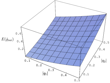
FIG. 2.: Entanglement produced at a lossless $50\%/50\%$ beam splitter by mixing two modes prepared in squeezed vacuum states as a function of $|q_{1}|$ and $|q_{2}|$ for the phase condition $2(\phi_{R}$ $\!-$ $\!\phi_{T})$ $\!+$ $\!\phi_{2}$ $\!-\phi_{1}$ $\!=$ $\!\pi$.

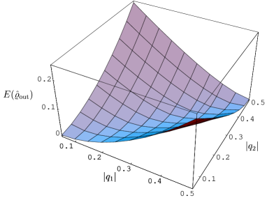
FIG. 3.: Entanglement produced at a lossless $50\%/50\%$ beam splitter by mixing two modes prepared in squeezed vacuum states as a function of $|q_{1}|$ and $|q_{2}|$ for the phase condition $2(\phi_{R}$ $\!-$ $\!\phi_{T})$ $\!+$ $\!\phi_{2}$ $\!-\phi_{1}$ $\!=$ $\!0$.

FIG. 4.: Entanglement produced at a lossless beam splitter with refractive index $n$ $\!=$ $\!1.41$ (dashed curve) as a function of the beam splitter thickness $l$. The full curve shows the upper bound of the produced entanglement at a lossy beam splitter with $n$ $\!=$ $\!1.41+0.1i$. The squeezing parameters chosen are $q_{1}$ $\!=$ $\!q_{2}$ $\!=$ $\!0.5$.

FIG. 5.: A two-mode input field prepared in the quantum state $|\psi\rangle$ is transmitted through two absorbing dielectric four-port devices, $\hat{a}_{1}$, $\hat{a}_{3}$ ($\hat{a}_{2}^{\prime}$, $\hat{a}_{4}^{\prime}$) being the photonic operators of the relevant input (output) modes.

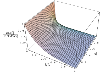
FIG. 6.: Estimate of the entanglement, Eq. (47), observed after transmission of a TMSV through absorbing fibers ($T_{1}$ $\!=$ $\!T_{2}$) as a function of the squeezing parameter $|q|^{2}$ and the transmission length $l$.

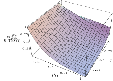
FIG. 7.: Upper bound on the entanglement degradation of a TMSV transmitted through absorbing fibers ($T_{1}$ $\!=$ $\!T_{2}$) as a function of the squeezing parameter $|q|$ and the transmission length $l$. In the numerical calculation, at most 30 photons per mode have been taken into account which is obviously not sufficient for higher squeezing when higher photon-number states are excited.

FIG. 8.: Upper bound of the entanglement degradation of a TMSV transmitted through absorbing fibers ($T_{1}$ $\!=$ $\!T_{2}$) as a function of the transmission length $l$ for the squeezing parameters $q$ $\!=$ $\!0.1$ (solid line) and $q$ $\!=$ $\!0.9$ (dashed line). In the numerical calculation, Fock states $|n\rangle$ up to $q^{n}$ $\!\lesssim$ $\!0.02$ have been taken into account.

FIG. 9.: Entanglement degradation of a TMSV transmitted through absorbing fibers ($T_{1}$ $\!=$ $\!T_{2}$) as a function of the transmission length $l$ for the (initial) mean photon numbers $\bar{n}$ $\!=$ $1$ ($|q|$ $\!\simeq$ $\!0.7071$) (topmost curve), $\bar{n}$ $\!=$ $10$ ($|q|$ $\!\simeq$ $\!0.9535$), $\bar{n}$ $\!=$ $10^{2}$ ($|q|$ $\!\simeq$ $\!0.9950$), and $\bar{n}$ $\!=$ $10^{3}$ ($|q|$ $\!\simeq$ $\!0.9995$) (lowest curve).

FIG. 10.: Available entanglement after transmission of a TMSV through absorbing fibers ($T_{1}$ $\!=$ $\!T_{2}$) as a function of the squeezing parameter $\xi$ for various transmission lengths $l$ [ $l$ $\!=$ $\!0$ (topmost curve), $l$ $\!=$ $\!10^{-2}l_{A}$ (middle curve), $l$ $\!=$ $\!10^{-1}l_{A}$ (lowest curve)]. For $|\xi|$ $\!\lesssim$ $\!0.5$ and $l/l_{A}$ $\!\lesssim$ $\!10^{-2}$, the numerical accuracy of the values of $E(\hat{\varrho}_{\rm out}^{\rm(F)})$ decreases due to low accuracy in the eigenvector computation.

FIG. 11.: Comparison of the upper bound on entanglement (upper curve) according to Fig. 7, the entanglement estimate (middle curve) according to Fig. 6, and the distance measure (lower curve) according to Fig. 9 for the mean photon number $\bar{n}$ $\!=$ $1$ ($|q|$ $\!\simeq$ $\!0.7071$).