Low energy atomic collision with dipole interactions

Abstract

We apply quantum defect theory to study low energy ground state atomic collisions including aligned dipole interactions such as those induced by an electric field. Our results show that coupled even ($l$) relative orbital angular momentum partial wave channels exhibit shape resonance structures while odd ($l$) channels do not. We analyze and interpret these resonances within the framework of multichannel quantum defect theory (MQDT).

34.50.-s, 34.50.Cf, 05.30.Jp, 05.30.Fk

I INTRODUCTION

Due to the tremendous progress made in laser cooling and trapping [1], cold atomic collision has become a frontier area of research in recent years. The atomic Bose-Einstein condensation demonstrations [2] have furthered this new trend of research in atomic physics. Recently, a topic of particular interest is the manipulation of BEC and matter- waves properties by controlling atom-atom interactions. Several groups have discussed mechanisms for changing the scattering length of atomic collision using near resonant lasers [3], radio frequency fields [4], Feschbach resonance due to a magnetic field [5], and shape resonance from dc electric field (dc-E) induced dipole interactions [6].

In this paper we present a detailed multichannel scattering investigation of low energy atomic collisions with anisotropic dipole collisions. Earlier studies of this problem [6, 7] have revealed several interesting features at low collision energies. Of particular interests to this study is its potential applications to modify (bosonic) atom-atom interaction strength with scattering resonances and the generation of p-wave BCS states for a single component fermi gas [7]. In this article, we develop a multichannel quantum defect theory (MQDT) using exact asymptotic solutions for the long range interatomic potential to analyze scattering resonance features. Our main aim is to explain the physical origin of dc-E dipole interaction induced resonances in the low energy limit. We also want to understand why such resonances only occur in even ($l$) partial wave channels, but not among odd ($l$) channels as numerically discovered earlier [6]. In a model study with two coupled channel ($l=0$ and $2$), we attempt to clarify the results of complicated multichannel scattering and illustrate the simple origin of these resonances. We find these are shape resonance caused by the coupling between different spatial spherical harmonic scattering channels due to anisotropic dipole interaction.

This paper is organized as follows; First we briefly discuss how an external dc-E modifies the effective interaction potential between two neutral atoms. We then present a detailed mathematical scattering formulation in Sec. II. In section III, we describe numerical techniques for the multichannel scattering calculation developed earlier by Marinescu and You [6], and present additional illustrative results (for ⁸⁵Rb in the singlet molecular potential state). The MQDT including dipole interaction is described in Sec. IV. In section V, we analyze the structure of the observed shape resonance with a simple model using only two (lowest angular momentum $l$) coupled channels. The dc-E field dependent zero energy bound states are discussed for the two channel model system in Sec. VI. Finally we summarize and conclude in Sec. VII.

II Formulation

The long-range interaction between two spherically symmetric atoms in the ground state, is usually given [in the London-van der Waals (LvW) formalism] by

$$V_{0}(R)=-\frac{C_{6}}{R^{6}}-\frac{C_{8}}{R^{8}}-\frac{C_{10}}{R^{10}}\cdots,$$ (1)

where $C_{6}$, $C_{8}$, and $C_{10}$ are the dispersion coefficients, and $R$ is the internuclear distance. With this asymptotic potential, zero energy scattering is described essentially only by one parameter: the s-wave scattering length, $a_{\rm sc}$ [8]. In the absence of a dc-E, the Hamiltonian of a model system of two spherically symmetric neutral alkali atoms A and B can be written as

$$H=H_{A}+H_{B}+V_{c}$$ (2)

where $H_{i=A,B}$ is the unperturbed Hamiltonian of atom $i$, and $V_{c}$ is the Coulomb potential between charge distributions of the two atoms and is given by the multipole expansion from [9]

$$V_{c}=\sum_{l,L=1}\frac{V_{lL}(\vec{r_{A}},\vec{r_{B}})}{R^{l+L+1}}$$ (3)

where $\vec{r_{i}}$ is the position vector of valence electron of $i$-th atom and $R$ is the separation between the centers of mass of the two atoms. Take the spatial quantization axis to be along the interatomic direction $\hat{R}$, the coefficient $V_{lL}(\vec{r_{A}},\vec{r_{B}})$ is then given by

$$V_{lL}=(-1)^{L}4\pi(\hat{l}\hat{L})^{-1/2}\sum_{m}{\mathbf{K}}_{lL}^{m}r_{A}^{l}r_{B}^{L}Y_{lm}(\hat{r}_{A})Y_{L-m}(\hat{r}_{B})$$ (4)

with $\hat{l}\equiv 2l+1$, $\hat{L}\equiv 2L+1$, and

$${\mathbf{K}}_{lL}^{m}=\left[C_{l+L}^{l+m}C_{l+L}^{L+m}\right]^{1/2},$$ (5)

where $C_{L}^{m}={L!}/[{m!(L-m)!}]$. Equation (1) of the long range dispersion is obtained from a perturbation calculation of $V_{c}$ in the limit of large $R$ when exchange effects between different atoms are negligible.

The presence of a dc-E distorts the spherical symmetry of an atom, consequently, the long-range form of interatomic potential Eq. (1) is modified. In the $R\rightarrow\infty$ limit, the ground state wave function $|S\rangle\equiv|n_{g},l=0,m=0\rangle$ ($n_{g}$, $l$, and $m$ are respectively the principal, angular, and magnetic quantum numbers) of an atom acquires a small $P$ angular momentum component due to the electric dipole coupling with excited states. Within the first order perturbation theory, the perturbed ground state wave function can be written as $|\phi\rangle=|S\rangle+{\cal E}|{\mathbf{P}}\rangle$, where $|{\mathbf{P}}\rangle$ is the sum of all $P$ excited states,

$$|{\mathbf{P}}\rangle=\frac{1}{\sqrt{3}}\sum_{n,m}|n,l,m\rangle\frac{(n,1|r|n_{g},0)(\hat{s}\cdot\hat{e}_{m}^{*})}{E_{n,1}-E_{n_{g},0}}.$$ (6)

$\hat{s}$ denotes the unit vector along the dc-E direction and $r$ is the valance electron coordinate (dipole operator) expanded in the tensor operator basis $\hat{e}_{m}$ of $\vec{r}_{i}$. The first order energy perturbation, i.e. interatomic interaction potential can then be written as

$$E^{(1)} = \langle\phi\phi|V_{c}|\phi\phi\rangle$$ (7)

$$= \left(\langle SS|+{\cal E}\langle S{\mathbf{P}}|+{\cal E}^{2}\langle{\mathbf{P}}{\mathbf{P}}|\right)V_{c}\left(|SS\rangle+{\cal E}|S{\mathbf{P}}\rangle+{\cal E}^{2}|{\mathbf{P}}{\mathbf{P}}\rangle\right).$$ (8)

To leading order in the dc-E amplitude $\cal E$, equation (8) generates an additional term,

$$V_{E}(R)=-\frac{C_{E}}{R^{3}}P_{2}(\cos\theta),$$ (9)

to the LvW formalism of Eq. (1). $C_{E}=2{\cal E}^{2}\alpha_{1}^{A}(0)\alpha_{1}^{B}(0)$ is the induced electric dipole interaction coefficient with $\alpha_{1}^{A(B)}(0)$ the static atomic dipole polarizabilities of atom A(B). $P_{2}(.)$ is the Legendre polynomial of order 2 and $\theta$ is the angle between the directions of the electric field ($\hat{s}$) and the internuclear axis ($\hat{R}$). As discovered earlier by Marinescu and You [6] this electric field induced dipole interaction Eq. (9), has a “quasi long-range” character in the sense that it generates a “short-range” contribution to the effective potential of the partial wave channel $l=0$ while it generates a “long-range” contribution (proportional to $-1/R^{3}$) for all other partial wave channels ($l\neq 0$).

Assuming a weak dc-E, the value of the induced dipole term [Eq. (9)] is small in comparison to typical atomic energy scale [e.g. 100 (kV/cm) is equivalent to $1.94401\times 10^{-5}$ (a.u.)]. Nevertheless, the qualitatively different asymptotic behavior for the interaction potential (i.e. $-1/R^{3}$) provides significant implications for threshold behaviors of low energy collision. We recall that for a spherically symmetric short range potential (which vanishes exponentially with increasing $R$), partial wave scattering phase shift obeys the Wigner threshold law $\delta_{l}(k)\sim k^{2l+1}$ at low energies. For a long range potential vanishes as $-1/R^{n}$, $\delta_{l}$ instead behaves in the limit of zero energy as $k^{2l+1}$ if $l<(n-3)/2$ and as $k^{n-2}$ otherwise [10]. For our problem, the complete long-range interatomic potential is given by $V_{0}(R)+V_{E}(R)$, where $V_{0}(R)$ is the usual long-range dispersion form Eq. (1) free of dc-E. Different partial wave channels are now coupled because of the anisotropic $Y_{20}(\hat{R})\sim P_{2}(\hat{R})$ in $V_{E}$. Applying the rule for low energy collision phase shifts to all diagonal terms of the potential, we discover the interesting situation where all partial wave phase shifts are proportional to $k$ due to the presence of induced dipole interaction $V_{E}$ [6].

The anisotropic Eq. (9) couples different angular momentum channels. The matrix elements for the scattering potential are simply

$$V(R)\delta_{ll^{\prime}}\delta_{mm^{\prime}}-\frac{C_{E}}{R^{3}}\langle lm|P_{2}(\cos\theta)|l^{\prime}m^{\prime}\rangle,$$ (10)

where $|lm\rangle=Y_{lm}(\hat{R})$ and $V(R)$ is the usual dc-E free isotropic interatomic potential which reduces to $V_{0}(R)$ in the large $R$ limit. Due to symmetry of the z-component of the angular momentum, the matrix element $\langle lm|P_{2}|l^{\prime}m^{\prime}\rangle$ vanishes if $l+l^{\prime}$ is an odd number; A non-zero coupling only exists if $l-l^{\prime}=\pm 2$ and $m=m^{\prime}$. Therefore even and odd parity channels as well as different $m$ blocks are decoupled.

Because of the coupling among different partial wave channels, the usual procedure for partial wave scattering calculation needs to be modified to accommodate the dipole interaction $V_{E}$. We assume the scattering wavefunction for $R\rightarrow\infty$ to be of the form

$$R\Psi(\vec{R})\sim R\exp(i\vec{k}\cdot\vec{R})+f(\vec{k},\hat{R})\exp(ikR)$$ (11)

where $\vec{k}$ is the incident momentum. The on-shell elastic scattering is then described by $f(\vec{k},\hat{R})$ with the scattered momentum $\vec{k}^{{}^{\prime}}=k\hat{R}$. We expand the scattering amplitude $f(\vec{k},\hat{R})$ onto the complete basis

$$f(\vec{k},\hat{R})=\frac{4\pi}{k}\sum_{lm}T_{lm}(\vec{k})Y_{lm}(\hat{R})$$ (12)

and apply the partial wave expansion

$$\exp(i\vec{k}\cdot\vec{R})=4\pi\sum_{l,m}i^{l}j_{l}(kR)Y_{lm}^{*}(\hat{k})Y_{lm}(\hat{R}).$$ (13)

We then obtain for $R\rightarrow\infty$

$$R\psi_{k}(\vec{R})=\phi_{k}(\vec{R})=\frac{4\pi}{k}\sum_{lm}i^{l}\left[Y_{lm}^{*}(\hat{k})\sin(kR-l\pi/2)+T_{lm}(\vec{k})\exp(ikR-il\pi/2)\right]Y_{lm}(\hat{R}),$$ (14)

where we have used the asymptotic form $j_{l}(kr)\sim\sin(kR-l\pi/2)/(kR)$. Therefore the scattering equations take the multichannel form

$$h_{l}\phi_{lm}(\vec{R})=\sum_{l^{\prime}m^{\prime}}i^{l^{\prime}-l}\langle lm|V(\vec{R})|l^{\prime}m^{\prime}\rangle\phi_{l^{\prime}m^{\prime}},$$ (15)

with

$$h_{l}=-\frac{\hbar^{2}}{2\mu}\frac{d^{2}}{dR^{2}}+\frac{\hbar^{2}}{2\mu}\frac{l(l+1)}{R^{2}}-E,$$ (16)

and $\phi_{lm}=\langle lm|R\Psi(\vec{R})\rangle$. $E=\hbar^{2}k^{2}/(2\mu)$ is the collision energy. The boundary conditions are then given by

$$\phi_{lm}\sim Y_{lm}^{*}(k)\sin(kR-l\pi/2)+T_{lm}(\vec{k})\exp(ikR-il\pi/2).$$ (17)

The above coupled multichannel scattering equation in relative angular momentum ($l$) channels can also be conveniently written in a matrix form

$$\left[(-\frac{\hbar^{2}}{2\mu}\frac{d^{2}}{dR^{2}}+V){\mathbf{I}}+\frac{\hbar^{2}}{2\mu R^{2}}{\mathbf{L}}^{2}+{\mathbf{V}}_{E}\right]{\mathbf{\Phi}}=E{\mathbf{\Phi}},$$ (18)

where $\mathbf{I}$ is the identity matrix, $\mathbf{L}$ is the momentum operator and ${\mathbf{L}}^{2}$ takes the form of a diagonal matrix: ${\mathbf{L}}^{2}={\mathbf{Diag}}[l(l+1),(l+2)(l+3),\cdots]$ with $l=$ even or odd channels decoupled; $\mu=M/2$ is the reduced mass for two identical atoms. The wave function ${\mathbf{\Phi}}$ is a column vector containing coupled channel function $\phi_{lm}$, (i.e., different outgoing channels $Y_{lm}(\hat{R})$). Since we need a complete set of linear independent scattering solutions to determine $T_{lm}$ from its expansion

$$\frac{1}{k}T_{lm}(\vec{k})=\sum_{l^{\prime}m^{\prime}}t_{lm}^{l^{\prime}m^{\prime}}(k)Y_{l^{\prime}m^{\prime}}(\hat{k}),$$ (19)

${\mathbf{\Phi}}$ is made to be a matrix with different columns characterizing scattering solutions for different incident channels $Y_{lm}(\hat{k})$. The T-matrix elements, $T_{lm}^{l^{\prime}m^{\prime}}$, can be extracted by imposing the boundary condition Eq. (17) on the partial waves in the asymptotic region. The total elastic cross section is given by

$$\sigma_{\rm E(O)}=8\pi\sum_{l,l^{\prime}={\rm even(odd)}}\sum_{m,m^{\prime}}|t_{lm}^{l^{\prime}m^{\prime}}|^{2}.$$ (20)

for E (even) and O (odd), respectively. We recall that $t_{lm}^{l^{\prime}m^{\prime}}=-a_{\rm sc}\,\delta_{l0}\delta_{l^{\prime}0}\delta_{m0}\delta_{m^{\prime}0}$ for spherically symmetric collisions described by Eq. (1) without the dipole interaction.

As a technical note for caution, we emphasize that the dipole interaction Eq. (9) is only valid for $R>\!>a_{0}$ ($a_{0}$ is Bohr radius). In constructing the complete potential, it is therefore required to be smoothly added to the isotropic potential, whose short range part $V_{\rm sh}$ also needs to be smoothly connected with its asymptotic form $V_{0}$. We used different cut-off radius $R_{c}$ with the same matching function for this purpose

$$f_{c}(R)=\theta(R-R_{c})+\theta(R_{c}-R)\exp[-(R_{c}/R-1)^{2}],$$ (21)

where $\theta(.)$ is the step function. We also note as elucidated by Jackson [11], an additional contact term is needed for the point dipole interaction to comply with the Gauss’s law. For our case of Eq. (9), this amounts to a contact term $-8\pi\alpha^{(A)}\alpha^{(B)}{\cal E}^{2}\delta(\vec{R})/3$. Such an addition is absent in our formulation since its effect is already implicitly included in the short range potential of $V(R)$.

III Results and Discussions

The standard numerov technique was adopted in numerically propagating Eq. (18) to obtain asymptotic scattering solutions. At lower energies, details of the potential functions $V(R)$ becomes important. Accurate potentials were obtained from other groups [12]. Most often we adopted a parametrization approach to adjust a reasonable $V_{\rm sh}$ potential such that a correct $a_{\rm sc}$ was obtained. To be able to solve the problem efficiently, we adopted a variable step size $h$ along $R$. With numerov we propagate from $R=0$ to asymptotic region $R_{\infty}$, we specify the initial conditions as ${\mathbf{\Phi}}(0)=0$ and ${\mathbf{\Phi}}(h)={\mathbf{\Phi}}_{\rm arb}$, where ${\mathbf{\Phi}}_{\rm arb}$ is an arbitrary symmetric matrix whose columns are chosen to be linearly independent vectors. In the absence of analytical solutions, there seems to be no clear-cut criteria for choosing the asymptotic region. With our numerical code, in the sub-$\mu K$ energy region, typically convergent results were only obtained for $R\geq 10^{7}a_{0}$. In order to maintain orthogonality and linear independence of different solution vectors during propagation, the subspace rotation technique is performed regularly. In the asymptotic region, we determine (by matching to potential free motion states)

$$\phi_{lm}=c_{1}\sin(kR-l\pi/2)+c_{2}\cos(kR-l\pi/2),$$ (22)

and construct the S-matrix with its element given by $(c_{1}-ic_{2})^{-1}(c_{1}+ic_{2})$ and the T-matrix $({{\mathbf{S}}-1})/{(2i)}$.

In the illustrative study to be reported below, unless stated otherwise, we always use ⁸⁵Rb atoms in its singlet potential curve. We have employed a maximum angular quantum momentum $l=8$ (9) for even (odd) channels, respectively. A reasonably good asymptotic radius $R_{\infty}$ is chosen to satisfy $|V-C_{3}/R^{3}|<10^{-6}\times|{\hbar^{2}l(l+1)}{R^{2}}/{(2\mu)}-E|$ with $l=2$ (1) for even (odd) partial wave channels.

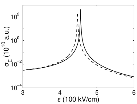
FIG. 1.: The total scattering cross section as a function of dc-E field ${\cal E}$ for several different cut-off radius $R_{c}=10(a_{0})$ (dashed line) and $R_{c}=27(a_{0})$ (solid line). Typically an increase of $R_{c}$ results in a shift to higher ${\cal E}$ value of the resonance peak at ${\cal E}_{r}$. Collision energy is $E=0.01$ (nk).

First, we discuss the choice of cut-off radius $R_{c}$ and the asymptotic radius $R_{\infty}$ for our numerical calculations. Figures 1, 2, and 3 illustrate effects of different values for electric dipole cut off radius $R_{c}$. In general, we find that resonance peak shifts towards higher ${\cal E}$ values as $R_{c}$ increases. Because of the perturbative nature for the effective long range dipole interaction, $R_{c}$ is always taken to be much larger than $a_{0}$. Unless otherwise stated, we will use $R_{c}=27(a_{0})$ to present our results. The small $R_{c}$ dependence can be operationally fixed by a normalization against any dc-E field dependent experimental data.

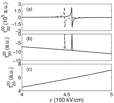
FIG. 2.: Selected reduced T-matrix elements under the same conditions as in Fig. 1. In (c), the two curves are indistinguishable.

Figure 2 shows that, among all partial wave channels, scattering in the s-wave ($l=0$) channel is the most sensitive with the choice of cut-off radius, while higher $l$ channel results remain almost unaffected. Physically this $R_{c}$ dependence can be explained in terms of the centrifugal potential term $\propto l(l+1)/R^{2}$ which is absent for the s-wave channel. Comparing with Fig. 1, we see that the resonance at ${\cal E}=456$ (kV/cm) is mostly due to the contribution from $t_{00}^{00}$ (s-wave) despite the anisotropic nature of dc-E induced dipole interaction. The coupling of s- to d-wave is the main reason for such a resonance as otherwise there seems no direct dipole interaction contributions to the s-wave channel. Our extensive calculations show that typical values of $t_{00}^{20}$ are many orders of magnitude smaller than $t_{00}^{00}$ [for ${\cal E}<1$ (MV/cm)]. This is explicitly shown in Fig. 3, where the ratio for different partial wave cross sections are compared with the s-wave one. We see that at low energies, scattering cross section for $l>2$ channels are smaller than that for the s-wave ($l=0$) by at least two orders of magnitude for ${\cal E}<1$ (MV/cm). At and near the resonance, scattering for $l\neq 0$ are absolutely negligible ($<10^{-5}$ of $\sigma_{00}^{00}$) in this case.

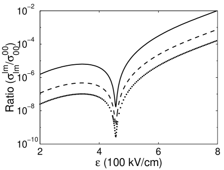
FIG. 3.: The high $l$ channel partial wave scattering cross sections are compared to the s-wave cross section in terms of the ratios $\sigma_{20}^{20}/\sigma_{00}^{00}$ (solid line), $\sigma_{30}^{30}/\sigma_{00}^{00}$ (dashed line), and $\sigma_{40}^{40}/\sigma_{00}^{00}$ (dotted line) at $E=0.01$ (nk).

For ${\cal E}<200$ (kV/cm), we find the $R_{c}$-dependence to be marginal as shown in Fig. 4. But at increased field strength the overall effect is not always negligible ($>1$%).

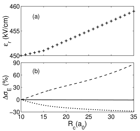
FIG. 4.: The dependence of the resonance value ${\cal E}_{r}$ (a) and the percentage change of the total scattering cross section (b) on $R_{c}$ at a selected dc-E values of ${\cal E}=200$ (kV/cm) (solid line), ${\cal E}=500$ (kV/cm) (dashed line), and ${\cal E}=1000$ (kV/cm) (dotted line). $E=0.01$ (nk).

Next, we consider the low energy threshold dependence of the scattering cross section. As discussed earlier, we expect the asymptotic behaviour $T_{lm}^{l^{\prime}m^{\prime}}\sim k$ at sufficiently low energies. We have performed extensive calculations to assure that all reported results are asymptotically converging such that we indeed have reached this limit. In Fig. 5 we display the variation of total scattering cross section $\sigma_{E}$ as a function of energy ranging from nK to mK regime. We see that for ${\cal E}=100$ (kV/cm), $\sigma_{E}$ becomes almost independent of energy below 1 ($\mu$K), while at ${\cal E}=456$ (kV/cm) $\sigma_{E}$ varies almost linearly with inverse of energy in the range of $20$ (nK) to $10$ ($\mu$K). It is worth pointing out here that at ${\cal E}=456$ (kV/cm), a resonance occurs at low energy as discussed later resulting in a divergent low energy cross section $\propto 1/k^{2}$.

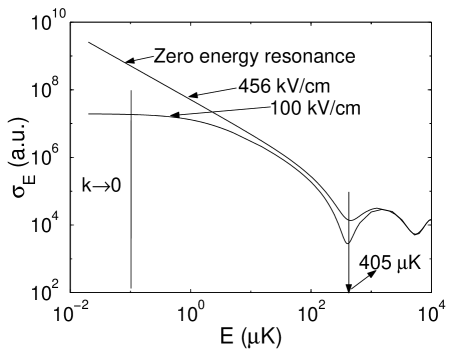
FIG. 5.: The dependence of zero energy scattering cross section ($\sigma_{E}$) on collision energy for selected dc-E values of ${\cal E}=100$ (kV/cm) and ${\cal E}=456$ (kV/cm). At any zero energy resonance, the scattering cross sections scales inverse proportional to collision energy.

Figure 6 is a selected result from odd ($l$) partial wave channels for ⁸²Rb (fermion). No resonance structure was ever detected in such cases.

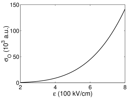
FIG. 6.: An example of the total scattering cross section $\sigma_{O}$ for ⁸²Rb (fermion) is also found to be dominated by $t_{10}^{10}$. No resonance occurs in this case, and $E=0.01$ (nk).

In Fig. 7, we plot the scattering cross section of ⁸⁵Rb for large fields ${\cal E}>1$ (MV/cm). As the field strength increases the resonance become more closely spaced. Again, the major contribution to the scattering comes from s-wave channel, although increased coupling between s- and higher $l$- partial waves with field strength is responsible for the multiple peak resonance structure.

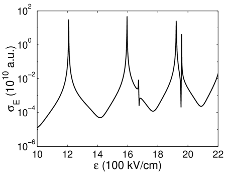
FIG. 7.: The dc-E field ${\cal E}$-dependent total scattering cross section of ⁸⁵Rb at a collision energy $E=0.01$ (nK). Multiple resonance structures appear in this case for ${\cal E}>1$ (MV/cm).

The results presented so far are obtained by radial integrations of coupled Schröedinger equations. There are certain practical disadvantages of using such a exclusively numerical method. First, it takes considerable amount of time to obtain the results, since the propagation of solutions continue until the asymptotic radius, which can be of the order of $10^{7}a_{0}$ or higher, is reached. The lower the energy, the longer the cpu time is needed because of increased $R_{\infty}$; Second, the increase of either collision energy or dc-E field strength or both calls for reduced propagation step size which again prolongs numerical computations; Third, as discussed earlier, the asymptotic boundary is not well defined. Therefore, no direct physical insight is gained about the resonance. In order to overcome these shortcomings of the numerical method, we have developed a MQDT for scattering with anisotropic dipole interactions. Quantum defect theory (QDT) relies on matching numerically integrated scattering solutions to analytic solutions (not asymptotic plane waves). The integration can be restricted to much shorter radius $R$ if appropriate analytical solutions are known. This not only makes the computation faster, the use of analytical solutions to the long range potential also helps to gain deep insight into resonance phenomena and low energy threshold behaviour.

IV Quantum defect theory for anisotropic dipole interaction

Quantum defect theory [13] was originally formulated to explain the spectrum of hydrogenic Rydberg atoms. In the Rydberg’s formula, $E_{n}=-R/(n-\mu)^{2}$ where $R$ is the Rydberg constant; the quantum defect $\mu$ accounts for effects of the ionic core on a highly excited electron. The idea of QDT has been successfully applied in atomic collisions and spectroscopy over the years [13]. The multichannel version of QDT, known as MQDT provides a good theoretical framework for analysis of diverse phenomena in atomic and molecular physics. In collision theory, MQDT requires analytical solutions in all asymptotic channel potentials. In the present problem including anisotropic dipole interaction, the diagonal elements of potential matrix goes asymptotically as $-1/R^{n}$ with $n=6$ for $l=0$ and $n=3$ for all other channels ($l\neq 0$). The exact solutions of these power law potentials have only recently become available through application of secular perturbation method [14, 15].

We first consider $n$ channels, as noted earlier, of even ($l$) angular momentum scattering states. In the asymptotic region, the diagonal potential term for s-wave channel $l=0$ goes as $-1/R^{6}$ while the diagonal terms for $l>0$ channels varies as $-1/R^{3}$. Applying MQDT, we first numerically integrate the multi-channel scattering equation (18) from $R=0$ to a certain $R=R_{0}$ such that $C_{6}/R_{0}^{6}<\!<|\langle 20|V_{E}(R_{0})|20\rangle|$. How to make a judicious choice of $R_{0}$ will be discussed later. Next, as a first approximation, we neglect off-diagonal potential terms for $R>R_{0}$. We note more complicated procedure exists that can incorporate off-diagonal effects in the long-range regime ($R>R_{0}$) [16]. It will be discussed later. The exact solutions of $-1/R^{6}$ and $-1/R^{3}$ potentials are then matched to numerically integrated multi-channel wave functions at $R_{0}$ in the spirit of MQDT

$${\mathbf{\Phi}}={\mathbf{I\,F}}+{\mathbf{J\,G}},$$ (23)

where

$${\mathbf{F}} ={\mathbf{Diag}}[f^{(6)}_{l=0},f^{(3)}_{l=2},\cdots f^{(3)}_{l=2(n-1)}],$$ (24)

$${\mathbf{G}} ={\mathbf{Diag}}[g^{(6)}_{l=0},g^{(3)}_{l=2}\cdots g^{(3)}_{l=2(n-1)}],$$ (25)

are two diagonal matrices with $f^{(n)}_{l}$ and $g^{(n)}_{l}$ two suitably chosen linear independent base functions for $-C_{n}/R^{n}$ type potential. One can define a characteristic length scale for such a power law potential $\beta_{n}=(2\mu C_{n}/\hbar^{2})^{1/(n-2)}$. Explicit expressions for $f_{l}^{n}$ and $g_{l}^{n}$ are reproduced in appendix-A. Their asymptotic forms are given in appendix-B, which for $E>0$ are grouped as

$$\left(\begin{array}[]{cc}f_{l}^{(n)}(R\rightarrow\infty)\\ g_{l}^{(n)}(R\rightarrow\infty)\end{array}\right)=\left(\begin{array}[]{cc}Z_{fb}^{(nl)}&Z_{fc}^{(nl)}\\ Z_{gb}^{(nl)}&Z_{gc}^{(nl)}\end{array}\right)\left(\begin{array}[]{cc}\sin(kR-\frac{l\pi}{2})\\ \cos(kR-\frac{l\pi}{2})\end{array}\right).$$ (32)

The coefficient matrices $\mathbf{I}$ and $\mathbf{J}$ are determined by use of the Wronskians: ${\mathbf{I}}=W({\mathbf{\Phi}},{\mathbf{G}}){\pi}/{2}$ and ${\mathbf{J}}=-W({\mathbf{\Phi}},{\mathbf{F}}){\pi}/{2}$ at $R=R_{0}$. As a convention, we set the constant Wronskian $W(f_{l}^{(n)},g_{l}^{(n)})$ for the linear independent base pairs $f_{l}^{(n)}$ and $g_{l}^{(n)}$ to $2/\pi$. Substituting for the asymptotic form Eq. (32), we arrive at

$${\mathbf{F}}(R\rightarrow\infty) ={\mathbf{Z}}_{FB}{\mathbf{B}}+{\mathbf{Z}}_{FC}{\mathbf{C}},$$ (33)

$${\mathbf{G}}(R\rightarrow\infty) ={\mathbf{Z}}_{GB}{\mathbf{B}}+{\mathbf{Z}}_{GC}{\mathbf{C}},$$ (34)

where ${\mathbf{Z}}_{FB(C)}$ are $n\times n$ diagonal matrices of the form ${\mathbf{Diag}}[Z_{fb(c)}^{(60)},Z_{fb(c)}^{(32)},\cdots]$ and similarly expressions for ${\mathbf{Z}}_{GB(C)}$ with the subscript $F$ ($f$) replaced by $G$ ($g$). ${\mathbf{B}}={\mathbf{Diag}}[\sin(kR),\cdots,\sin(kR-{l\pi}/{2}),\cdots]$ and ${\mathbf{C}}={\mathbf{Diag}}[\cos(kR),\cdots,\cos(kR-{l\pi}/{2}),\cdots]$ are also diagonal matrices. Substituting these expressions into Eq. (23), we obtain

$${\mathbf{\Phi}}(R\rightarrow\infty) =({\mathbf{I}}\,{\mathbf{Z}}_{FB}+{\mathbf{J}}\,{\mathbf{Z}}_{GB}){\mathbf{B}}$$ (36)

$$+({\mathbf{I}}\,{\mathbf{Z}}_{FC}+{\mathbf{J}}\,{\mathbf{Z}}_{GC}){\mathbf{C}}.$$

From which we find the scattering K-matrix as

$${\mathbf{K}}=({\mathbf{Z}}_{FB}+{\mathbf{K}}^{0}{\mathbf{Z}}_{GB})^{-1}({\mathbf{Z}}_{FC}+{\mathbf{K}}^{0}{\mathbf{Z}}_{GC}),$$ (37)

where ${\mathbf{K}}^{0}={\mathbf{I}}^{-1}{\mathbf{J}}$ is a matrix that hopefully will depend only on shorter range interactions ($R\leq R_{0}$). In general, ${\mathbf{K}}^{0}$ will have some $R$ dependence. For the case of a single channel, it becomes a slowly varying function of $R$ and approaches a constant at $R_{0}$ where the potential attains its power law asymptotic form ($-1/R^{n}$). The matching point $R_{0}$ is therefore appropriately chosen such that ${\mathbf{K}}^{0}$ becomes independent of $R$. This is always possible as all analytic dependence on potential and collision energy is taken care of by the various ${\bf Z}$ functions. For multi-channel with anisotropic interactions as in the present context, the situation become more complicated, and will be discussed in the next section.

The S-matrix is obtained from K-matrix according to ${\mathbf{S}}=({\mathbf{1}}-i{\mathbf{K}})^{-1}({\mathbf{1}}+i{\mathbf{K}})$. The eigen phase shifts can be directly calculated from the diagonalized S-matrix ${\mathbf{\Lambda}}^{-1}{\mathbf{S}}{\mathbf{\Lambda}}={\mathbf{Diag}}[\exp(2i\delta_{0}),\exp(2i\delta_{2}),\cdots]$, where $\mathbf{\Lambda}$ is the unitary transformation matrix. Thus the phase shifts for different incoming and outgoing channels become available.

For odd ($l$) coupled partial wave channels, essentially the same mathematical structure as the above formalism remains, except now all diagonal potential terms are $\propto-1/R^{3}$ at large $R$. Therefore we only need analytical channel solutions for $-1/R^{3}$ type potential. This makes the odd angular momentum channel problem qualitatively different (simpler).

Before developing a model two channel problem, we briefly summarize a technique that would allow for inclusion of off-diagonal potential terms for $R>R_{0}$ within our approach [16]. In the presence of off diagonal couplings at large interatomic separation $(R>R_{0})$, the wavefunction for each channel $l$ can be expressed as

$$\phi_{l}=u_{l}(R)f_{l}(R)-v_{l}(R)g_{l}(R),$$ (38)

where $f_{l}$ and $g_{l}$ are the two linearly independent base functions as defined earlier satisfying the Schrödinger equation for a $-1/R^{n}$ type potential. We will suppress the $m$ quantum number index since even anistropic dipole potential $V_{E}$ remains diagonal in $m$. $u_{l}$ and $v_{l}$ are two slowly varying functions of $R$ defined by equations

$$\frac{d\phi_{l}}{dR} = u_{l}(R)\frac{df_{l}(R)}{dR}-v_{l}(R)\frac{dg_{l}(R)}{dR},$$ (39)

and

$$\frac{du_{l}}{dR} = \xi_{l}(R)g_{l}(R),$$ (40)

$$\frac{dv_{l}}{dR} = \xi_{l}(R)f_{l}(R).$$ (41)

By substituting the above expressions into the Schroedinger equation (16), we obtain

$$-W(f_{l},g_{l})\xi_{l}(R)=\frac{2\mu}{\hbar^{2}}\sum_{l^{\prime}\neq l}(i)^{l^{\prime}-l}(V_{E})_{ll^{\prime}}\phi_{l^{\prime}}(R)$$ (42)

where $W(f_{l},g_{l})$ is the Wronskian of the base pair $f_{l}$ and $g_{l}$. The solutions of Eq. (41) can then be written as

$$u_{l}(R) = u_{l}(R_{0})+\frac{\mu\pi}{\hbar^{2}}\int_{R_{0}}^{R}dR^{\prime}g_{l}(R^{\prime})\sum_{l^{\prime}\neq l}(i)^{l^{\prime}-l}(V_{E})_{ll^{\prime}}\phi_{l^{\prime}}(R^{\prime}),$$ (43)

$$v_{l}(R) = v_{l}(R_{0})+\frac{\mu\pi}{\hbar^{2}}\int_{R_{0}}^{R}dR^{\prime}f_{l}(R^{\prime})\sum_{l^{\prime}\neq l}(i)^{l^{\prime}-l}(V_{E})_{ll^{\prime}}\phi_{l^{\prime}}(R^{\prime}),$$ (44)

a form that allows for direct perturbation analysis [13]. The scattering matrix can be determined by evaluating values of $u_{l}$ and $v_{l}$ at large $R$ values, since the asymptotic expressions for $f_{l}$ and $g_{l}$ as given by Eq. (32) are known. The values of $u_{l}(R_{0})$ and $v_{l}(R_{0})$ are given by the condition that at $R=R_{0}$ the $l$-channel wave function $\phi_{l}$ given by Eq. (38) should coincide with the corresponding wave function given by Eq. (23). Thus $u_{l}(R_{0})$ and $v_{l}(R_{0})$ are then respectively elements of the matrices ${\mathbf{I}}$ and $-{\mathbf{J}}$. We will, however, not pursue such a complicated calculation as it turns out that most of the interesting physics in low energy dipole collision can be obtained through a simpler model calculation involving only two channels.

V two coupled channels

To illustrate the physics of dc-E induced shape resonance, we apply the MQDT method as outlined above, to a closed system of two coupled channels ($l=0$ and $2$). Given the fact that scattering for $l>2$ channels are almost negligible at low energies as illustrated in Fig. 3 for ${\cal E}$ field range of interests to us, this $2\times 2$ coupled-channel system represents a well justified model. From Eq. (18) we have,

$$\left[\left(-\frac{\hbar^{2}}{2\mu}\frac{d^{2}}{dR^{2}}+V-E\right)\left(\begin{array}[]{cc}1&0\\ 0&1\end{array}\right)+\frac{\hbar^{2}}{2\mu R^{2}}\left(\begin{array}[]{cc}0&0\\ 0&6\end{array}\right)-\frac{C_{E}}{R^{3}}\left(\begin{array}[]{cc}0&C_{20}\\ C_{20}&C_{22}\end{array}\right)\right]\left(\begin{array}[]{cc}\phi_{00}\\ \phi_{20}\end{array}\right)=0,$$ (53)

where $C_{ll^{\prime}}=\langle l0|P_{2}(.)|l^{\prime}0\rangle$. As $R\rightarrow\infty$, the diagonal potential terms in the channels $l=0$ and $l=2$ become $V_{0}=-C_{6}/R^{6}$ and $V_{2}\simeq{6\hbar^{2}}/{(2\mu R^{2})}-C_{E}C_{22}/R^{3}$, respectively. We, therefore, employ exact solutions of $-1/R^{6}$ and $-1/R^{3}$ potentials as obtained by B. Gao [14] to match numerically computed ones at a radius $R_{0}$. We first choose $R_{0}$ to satisfy condition $C_{6}/R_{0}^{6}<\!<C_{E}C_{22}/R_{0}^{3}$, i.e., $R_{0}>\!>[C_{6}/(C_{E}C_{22})]^{1/3}$. Therefore, as discussed in the previous section, we expect the diagonal element of ${\mathbf{K}}^{0}$ in the $l=2$ channel, i.e., $K^{0}_{22}$ should approach a constant as $R\rightarrow R_{0}$, provided the strength of the long range anisotropy is negligible for $R>R_{0}$. A good measure of the relative strength of the anisotropy can be defined according to

$$\eta(R)=\left|\frac{V_{12}}{V_{2}-V_{0}}\right|.$$ (54)

We neglect anisotropic effects for $R>R_{0}$ if $\eta(R>R_{0})$ drops well below unity (typically at $5\times 10^{-3}$). In Fig. 8 we have plotted $\eta$ as a function of $R$ for several different values of ${\cal E}$ field.

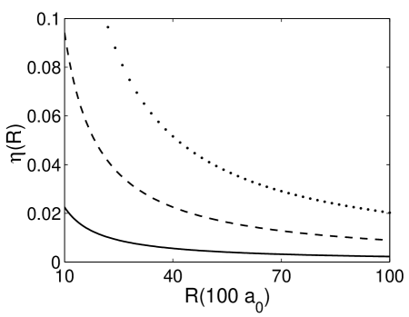
FIG. 8.: The strength of anisotropy versus $R$ for dc-E values of ${\cal E}=100$ (kV/cm) (solid line), ${\cal E}=1000$ (kV/cm) (dashed line), and ${\cal E}=1500$ (kV/cm) (dotted line).

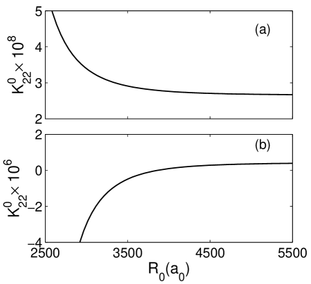
FIG. 9.: The variation of short-range K-matrix element $K_{22}^{0}$ as a function of $R$ for dc-E values of ${\cal E}=500$ (kV/cm) (a) and ${\cal E}=1000$ (kV/cm) (b) at a collision energy $E=1$ (nK).

In Figure 9, we display variations of $K^{0}_{22}$ as a function of $R_{0}$ for two different electric field strength at $1$ (nK) collision energy. We note that $K^{0}_{22}$ approaches a constant for $R\geq 4000(a_{0})$. The same behavior is true at even higher ${\cal E}$ fields, albeit, at still larger values of $R_{0}$. Therefore for ${\cal E}\leq 1000$ (kV/cm), we expect little loss of accuracy by neglecting off-diagonal terms when $R\geq 4000(a_{0})$. Based on the MQDT formulation discussed in the previous section, we have computed the scattering wave function as well as the corresponding T-matrix for our model of two coupled channels. In Figure 10, we show the scattering cross section as a function of dc-E field strength ${\cal E}$ at three different collisions energies. We note that the resonance becomes more prominent as collision energy is lowered below ($\mu$K), indicating the presence of a bound state or a virtual bound-state (quasi-bound) near the zero energy threshold. This calculation illustrates that our model indeed captures the resonance at ${\cal E}=456$ (kV/cm) as previously discussed in Fig. 5. This results are almost indistinguishable from a complete numerical calculations done earlier. We will discuss in more detail such zero energy resonances in the next section.

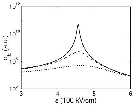
FIG. 10.: The dc-E field dependent scattering cross section $\sigma_{E}$ at three different collision energies $E=1$ (nK) (solid line), $E=100$ (nK) (dashed line), and $E=1$ ($\mu$K) (dotted line). These results are obtained by the MQDT method for two coupled channels.

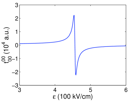
FIG. 11.: The reduced T-matrix element $t_{00}^{00}$ obtained by MQDT for two coupled channels ($l=0,2$) at $E=1$ (nK). This result is in fact indistinguishable from a numerical (two channel) calculation, although differs slightly from a multi-channel (five channel) calculation.

As a check of consistency, we note that results obtained from the MQDT two channel model calculation agree quite well with those obtained by the complete numerical calculations as long as the two channel approximation remains valid for ${\cal E}<1$ (MV/cm). For ${\cal E}>1$ (MV/cm), off-diagonal terms of the dipole potential are not negligible for the same value of MQDT matching radius $R_{0}$ used. A simple way of including more effects of off-diagonal terms would be to increase $R_{0}$. We therefore conclude that the MQDT does provide significant computational advantage over the direct numerical integration technique. It is especially efficient at lower energies when $E<10$ ($\mu$K).

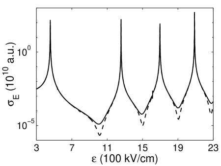
FIG. 12.: Comparison of numerical (dashed line) and MQDT (solid line) scattering cross sections within the two channel approximation for large dc-E fields (${\cal E}>1$ (MV/cm) at $E=0.01$ (nK). With such large electric fields, short range K-matrix only become independent of $R_{0}$ at rather large values, taken here to be $10000(a_{0})$.

We now analyze the long range behaviour of our two channel model. For the $l=0$ channel, the diagonal potential behaves asymptotically as $-1/R^{6}$. This singlet potential in fact can support many many bound states, including those close to the zero energy threshold [17]. For $l\neq 0$ channels, on the other hand, quasi-bound states (virtual bound states in the quasi-continuum) may also occur due to the presence of the centrifugal potential barrier. In the zero energy limit, scattering is mostly due to s-wave ($l=0$) in the regime of parameters of interest to us. Any alteration of the long-range s-wave potential ($-1/R^{6}$) due to electric-field-induced coupling with d-wave leads to a modification of its bound (quasibound) spectrum near the zero energy threshold. The effective potential $V_{2}$ (diagonal term plus centrifugal barrier) has a maximum (barrier) at $R=R_{m}$ given by the condition $dV_{2}/dR=0$, i.e. $R_{m}=\mu C_{E}C_{22}/(2\hbar^{2})$ and the barrier height is given by $\delta V=\hbar^{2}/(\mu R_{m}^{2})$. Since coefficient $C_{E}$ is proportional to field intensity ${\cal E}^{2}$, $R_{m}$ is linearly proportional to ${\cal E}^{2}$. Consequently, the barrier height becomes inversely proportional to ${\cal E}^{4}$. The coupling between s- and d-wave channels may lead to combined new bound or quasi-bound states or both at near-zero energies. The existence of these states is manifested in the form of scattering resonance. For instance when an incident low energy atom from s-wave channel hits a quasi-bound states supported by the d-wave centrifugal barrier, we may have a situation resemble what is commonly known as a Feshach resonance [5]. If there exists a bound state at or near zero energy, scattering cross sections will consequently be enhanced many-fold. This is indeed the case found in our earlier extensive numerical calculations. As will be proven in the next section on bound states, such resonance structures can be fully explained based on zero energy bound states using the MQDT.

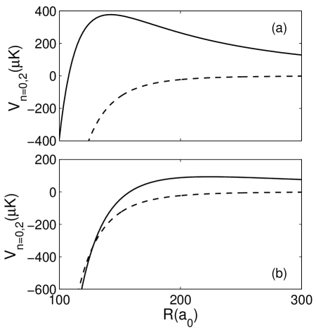
FIG. 13.: The diagonal potential terms $V_{0}$ (dashed line) for $l=0$ and $V_{2}$ (solid line) for $l=2$ at two different dc-E field strength ${\cal E}=456$ (kV/cm) (a) and ${\cal E}=1500$ (kV/cm) (b). The larger the ${\cal E}$ field, the further out in $R$ where the two potential curves crosses. The height of the $V_{2}$ potential barrier decreases with increasing ${\cal E}$.

VI Bound states

As discussed in the previous section, low energy scattering resonance is a signature of a bound or quasibound state near zero energy. At some critical dc-E field strength, a new bound state is formed at micro- or submicro-Kelvin energy leading to the observed zero-energy shape resonance. In order to elucidate this point explicitly, we again rely on the two-channel model and find its last bound or quasibound state just below zero energy by the MQDT formulation. The asymptotic form of linearly independent base pairs $f_{l}^{(n)}$ and $g_{l}^{(n)}$ satisfying the Schroedinger equation with a potential $-1/R^{n}$ for $E<0$ can be expressed as

$$\left(\begin{array}[]{cc}f_{l}^{(n)}(R\rightarrow\infty)\\ g_{l}^{(n)}(R\rightarrow\infty)\end{array}\right)=\left(\begin{array}[]{cc}W_{f-}^{(nl)}&W_{f+}^{(nl)}\\ W_{g-}^{(nl)}&W_{g+}^{(nl)}\end{array}\right)\left(\begin{array}[]{cc}\exp(\kappa R)\\ \exp(-\kappa R)\end{array}\right),$$ (61)

where $W$’s are chosen to be real functions. For the two coupled channels discussed in the previous section, we have

$$W_{f-}^{(60)} = (4\pi\kappa)^{-1/2}[(X_{0}^{2}+Y_{0}^{2})\sin(\pi\nu)]^{-1},$$ (62)

$$\times \left[\{\beta\sin(\pi\nu)+\alpha\cos(\pi\nu)\}G(-\nu)-\alpha G(\nu)\right],$$ (63)

$$W_{g-}^{(60)} = (4\pi\kappa)^{-1/2}[(X_{0}^{2}+Y_{0}^{2})\sin(\pi\nu)]^{-1}$$ (64)

$$\times \left[\{\alpha\sin(\pi\nu)-\beta\cos(\pi\nu)\}G(-\nu)+\beta G(\nu)\right],$$ (65)

and

$$W_{f-}^{(32)} = 2(2\pi\kappa)^{-1/2}\left[\frac{C_{+}(-\nu)}{G(-\nu)}\Delta^{\nu}-\frac{C_{+}(\nu)}{G(\nu)}\Delta^{-\nu}\right],$$ (66)

$$W_{g-}^{(32)} = 2(2\pi\kappa)^{-1/2}\left[-\frac{C_{-}(-\nu)}{G(-\nu)}\Delta^{\nu}+\frac{C_{-}(\nu)}{G(\nu)}\Delta^{-\nu}\right].$$ (67)

Except for $\hbar^{2}\kappa^{2}/(2\mu)=-E$, all notations used here follow from earlier definitions as in appendix-A. After some tedious algebra, the condition for bound states of our two channel model becomes

$${\rm Det}[{\mathbf{Q}}+{\mathbf{K}}^{0}]=0,$$ (68)

where ${\mathbf{Q}}$ is a diagonal matrix given by

$${\mathbf{Q}}={\bf Diag}[W_{f-}^{(60)},W_{f-}^{(32)}]\left({\bf Diag}[W_{g-}^{(60)},W_{g-}^{(32)}]\right)^{-1}.$$ (69)

The bound state wave function at discrete energy $E_{i}$ can then be expressed as

$$\Psi_{i}(R)=({\mathbf{F}}+{\mathbf{K}}^{0}{\mathbf{G}})M,$$ (70)

where ${\mathbf{F}}$, ${\mathbf{G}}$, and ${\mathbf{K}}^{0}$ are similar to matrices defined in Sec. IV, and $M$ is a column vector. Using the asymptotic form of base pairs functions, Eq. (70) can be rewritten as

$$\Psi_{i}(R\rightarrow\infty)=\exp(-\kappa R){\mathbf{Q}}_{+}M+\exp(\kappa R){\mathbf{Q}}_{-}M,$$ (71)

where

$${\mathbf{Q}}_{\pm}={\bf Diag}[W_{f\pm}^{(nl)},W_{f\pm}^{(n^{\prime}l^{\prime})},\cdots]+{\mathbf{K}}^{0}{\bf Diag}[W_{g\pm}^{(nl)},W_{g\pm}^{(n^{\prime}l^{\prime})},\cdots],$$ (72)

The bound state energy is therefore given by the requirement that the exponentially rising part of Eq. (72) vanishes, i.e.,

$${\rm Det}[Q_{-}]=0.$$ (73)

The matching radius $R_{0}$ in this case is chosen to be in classically allowed region of diagonal channel potentials. The condition for the existence of a new bound state, i.e. Eq. (68) is then given by

$$(Q_{11}+K^{0}_{11})(Q_{22}+K^{0}_{22})-K^{0}_{12}K^{0}_{21}=0,$$ (74)

where the subscript indices denote respective elements of ${\mathbf{Q}}$ and ${\mathbf{K}}^{0}$ matrices, and $(1/Q_{11})$ and $Q_{22}$ are the $\chi$ functions for a pure $-1/R^{6}$ or $-1/R^{3}$ potential as defined in Ref. [14]. Since the value of $K_{12}$ is typically much smaller than $K_{11}$ near resonance, as an approximation, we can drop the two off-diagonal elements from ${\mathbf{K}}^{0}$. We then obtain two uncoupled bound spectrum series, given respectively by

$$Q_{11}+K^{0}_{11}=0,$$ (75)

and

$$Q_{22}+K^{0}_{22}=0.$$ (76)

The first condition Eq. (75) gives bound states predominantly supported by s-wave channel. The effect of channel-coupling due to external electric field enters only through the parameter $K^{0}_{11}$. In this first approximation, the off-diagonal potential terms are neglected for $R>R_{0}$. As commented earlier, the short-range K-matrix ${\mathbf{K}}^{0}$ is a slowly varying function of collision energies near the zero energy threshold. We can then extrapolate their values from $E>0$ (for scattering) to the bound state case $E_{i}\leq 0$. In the present case of zero energy bound states satisfying $E_{i}\sim 0$, we basically used the same short range K-matrix as obtained from a converged low energy scattering calculation. We compute bound states near the zero energy threshold that satisfy

$$|E_{i}|<\!<C_{6}/R_{0}^{6}<C_{3}/R_{0}^{3}.$$ (77)

For an asymptotic $-1/R^{3}$ potential as in $l=2$, the matching radius $R_{0}$ is taken to be smaller than the characteristic length scale $\beta_{3}=2\mu C_{E}C_{22}/\hbar^{2}$ of the potential.

In Figure 14, we show the energy dependence of $Q_{11}^{-1}$. The last bound state of isolated s-wave $l=0$ channel (with asymptotic potential $-1/R^{6}$) is then given by crossing points of $Q_{11}$ and -$K_{11}^{0}$. In the absence of an external electric field, the energy of the last bound state supported by an asymptotic $-/R^{6}$ potential of ⁸⁵Rb is about $2$ (mK) which is in fact far beyond the zero energy limit appropriate for the present discussion. In the zero energy limit ($l=0$), $R_{0}$ can be taken arbitrarily large for the condition given by by the single channel bound state Eq. (75).

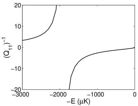
FIG. 14.: The inverse of $Q_{11}$ as a function of bound state energy in ($\mu$K) for ⁸⁵Rb.

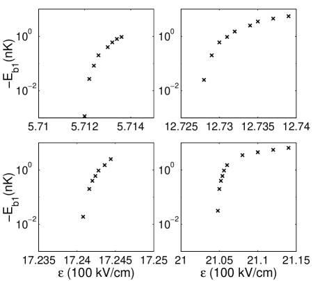
FIG. 15.: Bound state energies ($E_{b1}$) in the $l=0$ channel as a function of electric field ${\cal E}$ in the zero energy limit.

From Fig. 14, we see that a new zero energy bound state appears only when $K_{11}^{0}$ becomes infinite. In Fig. 15, we display variations of the subsequent four zero energy bound state energies as a function of ${\cal E}$. We used $K_{11}^{0}$ as determined at a positive energy near zero energy threshold and matched analytical solutions with the numerical ones at a relatively large $R$ ($R=4000a_{0}$ for ${\cal E}\!<1$ MV/cm, $R=10000a_{0}$ for ${\cal E}\!>1$ MV/cm). It is interesting to note that these resonances agree quite well with results obtained from a complete numerical multichannel scattering calculation presented before in Figs. 1 and 7.

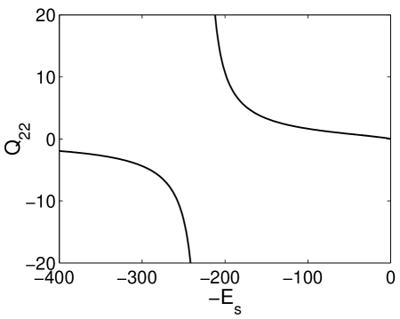
FIG. 16.: $Q_{22}$ as a function of scaled energy $E_{s}=2\mu C_{E}C_{22}E/\hbar^{2}$ for ⁸⁵Rb. For an asymptotic $-1/R^{3}$ potential as in the $l=2$ channel, use of this scaled energy helps to illustrate the long range interaction. The last bound state is given by crossing points of $Q_{22}$ with -$K^{0}$, just as in the $l=0$ s-wave case.

The second condition Eq. (76) corresponds to bound state series of the $l=2$ channel. In addition to dc-E effects accumulated in $Q_{22}$, the asymptotic wave function is now chosen to include the field induced diagonal term $\propto-1/R^{3}$. In Figure 16 we plot the energy and dc-E field dependent $Q_{22}$. It resembles $Q_{11}^{-1}$ rather than $Q_{11}$ because of a different choice between $g$ and $f$ functions. At field values of interest to us, we find the short-range ${\bf K^{0}}$ matrix actually changes rapidly in this case with the (relative small) matching radius $R_{0}$. Therefore, in the classically allowed region, we were not able to perform a correct MQDT with an energy and $R_{0}$ independent $K_{22}^{0}$. Nevertheless, to explore the physics qualitatively, we instead choose a radius $R_{0}=105(a_{0})$ (in the classically allowed region of the $l=2$ diagonal potential) such that it reproduces the first bound state as in the s-wave channel between ${\cal E}=500$ and $600$ (kV/cm). As we can see from Fig. 15, the third bound state then also seem to be reproduced correctly.

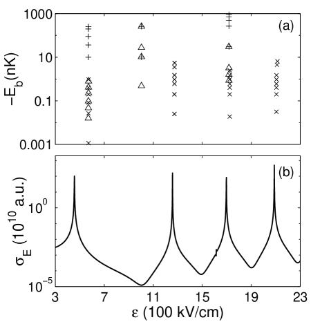
FIG. 17.: The comparison between zero energy bound states as obtained from MQDT for a single channel $l=0$ ($\times$), $l=2$ ($+$), and the two coupled channels ($\triangle$) in (a), and their comparison with numerical results from the two channel model (b). We note the s-wave single channel results matched in the classically forbidden region at $R_{0}\geq 4000(a_{0})$ reproduces exactly all numerically calculated scattering resonance. Note that the numerical two channel results here (b) differ somewhat from the complete multi-channel results given in Fig. 7.

We now proceed to estimate the combined bound state sequence by solving for Eq. (74). In this case, for bound state energy larger than a few $\mu$K, the classically forbidden region limits the choice of a matching radius to be within 100-150 $a_{0}$, which is much smaller than the typical value of 4000 $a_{0}$ used for the scattering calculations. We again choose the same matching radius at $105(a_{0})$ as for the single $l=2$ channel [Eq. (76)] discussed above. Obviously, there is no reason to trust the obtained results seriously as the neglected anisotropic effects become significant at such a small $R_{0}$. Nevertheless, it is interesting to compare the obtained results as in Fig. 17 for these three separate approximations. Note the comparison of bound state locations with the numerical calculated zero energy scattering cross section from the same two channel model. We find that the $l=0$ s-wave bound state locations match quite well with the numerically calculated resonance structures. This gives us the confidence to assign these resonances as due to dc-E field induced zero energy bound states, thus they are indeed shape resonance. As the strength of electric field is increased to a certain critical value, a new bound or quasibound state appears at the zero energy threshold. Since we neglect the off-diagonal potential terms for $R>R_{0}$, the bound state energies calculated here only provides approximate estimates, they differ from results reported in Fig. 8 obtained from a complete multichannel calculation. The fact that a single s-wave ($l=0$) channel completely captures the resonance structure is perhaps also not surprising, as it is indeed the dominant channel found numerically before. By choosing the matching radius $R_{0}$ to be sufficiently large, the anisotropic dipole induced coupling with other higher $l$ channels are included through the short range ${\bf K}^{0}$ matrix.

Finally we note that MQDT bound states technique used here may also be improved with a perturbative method as discussed earlier to include additional asymptotic ansiotropic effects [16].

VII Conclusion

We have presented a detailed analysis of low energy atomic collisions including electric field induced anisotropic dipole interaction. We have discussed both multichannel numerical and MQDT methods for the scattering calculations. In particular, we have highlighted the zero-energy resonance phenomena due to formation of long-range bound or quasi-bound states near the zero energy threshold. At low energies ($E\sim$ nK) and with reasonable dipole interaction strength, the scattering cross section is predominantly due to the s-wave for coupled even $l$ angular momentum channels. We also note that the zero energy resonance due to formation of new bound states only occurs in the coupled even $l$ channels, but not in the odd $l$ channels. This is mainly due to the presence of the s-wave potential well (without centrifugal potential) in the coupled even $l$ blocks. At positive energies, the s-wave channel is open throughout the entire range ($0<R<\infty$) of its diagonal potential, while other channels ($l>0$) have locally closed regions near zero energy. When s-wave is present, atoms can penetrate into shorter $R$ range via scattering and multichannel coupling and therefore zero-energy resonance is more likely to occur. By manipulating such scattering resonance with dc-E induced dipole interaction, it is possible to change low energy scattering properties such as the scattering length and total or partial wave scattering cross sections. In contrast to the magnetic field-induced Feshbach resonance where coupling between different hyper-fine levels (different internal states) are involved, electric field-induced resonance is due to coupling among different rotational (external) states of the two colliding atoms, and only one threshold (or internal state) is present in the system. In the present paper, using a model two channel MQDT calculation, we have provided a clear physical picture of these resonances and provided analytical means for estimating their locations. The availability of approximate analytical forms for these near zero-energy bound states allows for detailed examination of bound-free and free-free motional Franck-Condon factors.

A Analytic solutions for $-1/R^{n=3,6}$-type potential

The base pair for $-1/R^{6}$ potential is given by

$$f_{l}^{6} =\frac{1}{\sqrt{2}}(\alpha^{2}+\beta^{2})^{-1}[\alpha\tilde{f}_{l}(r)-\beta\tilde{g}_{l}(r)],$$ (A1)

$$g_{l}^{6} =\frac{1}{\sqrt{2}}(\alpha^{2}+\beta^{2})^{-1}[\beta\tilde{f}_{l}(r)+\alpha\tilde{g}_{l}(r)],$$ (A2)

where

$$\tilde{f}_{l}(r) =\sum_{m=-\infty}^{\infty}b_{m}r^{1/2}J_{\nu+m}\left(\frac{1}{2}(r/\beta_{6})^{-2}\right),$$ (A3)

$$\tilde{g}_{l}(r) =\sum_{m=-\infty}^{\infty}b_{m}r^{1/2}J_{\nu+m}\left(\frac{1}{2}(r/\beta_{6})^{-2}\right),$$ (A4)

with

$$\alpha =\cos[\pi(\nu-\nu_{0})/2]X_{l}-\sin[\pi(\nu-\nu_{0})/2]Y_{l},$$ (A5)

$$\beta =\sin[\pi(\nu-\nu_{0})/2]X_{l}+\cos[\pi(\nu-\nu_{0})/2]Y_{l},$$ (A6)

and

$$X_{l} =\sum_{m=-\infty}^{\infty}(-1)^{m}b_{2m},$$ (A7)

$$Y_{l} =\sum_{m=-\infty}^{\infty}(-1)^{m}b_{2m+1},$$ (A8)

and [14]

$$b_{j} =(-\Delta)^{j}\frac{\Gamma(\nu)\Gamma(\nu-\nu_{0}+1)\Gamma(\nu+\nu_{0}+1)}{\Gamma(\nu+j)\Gamma(\nu-\nu_{0}+j+1)\Gamma(\nu+\nu_{0}+j+1)}c_{j}(\nu),$$ (A9)

$$b_{-j} =(-\Delta)^{j}\frac{\Gamma(\nu-j+1)\Gamma(\nu-\nu_{0}-j)\Gamma(\nu+\nu_{0}-j)}{\Gamma(\nu+1)\Gamma(\nu-\nu_{0})\Gamma(\nu+\nu_{0})}c_{-j}(-\nu),$$ (A10)

where $j$ is a positive integer, $\Delta$ is a scaled energy, $\Delta=k^{2}\beta_{6}^{2}/16$ with $k=2\mu E/\hbar^{2}$; $\nu_{0}$ is related to the angular momentum $l$, $\nu_{0}=(2l+1)/4$, and $c_{j}(\nu)=b_{0}Q(\nu)Q(\nu+1)\cdots Q(\nu+j-1)$ with $b_{0}$ being a normalization constant; and $Q(\nu)$ is given by a continued fraction,

$$Q(\nu)={1\over 1-\Delta^{2}{1\over(\nu+1)(\nu+2)[(\nu+1)^{2}-\nu_{0}^{2}][(\nu+2)^{2}-\nu_{0}^{2}]}Q(\nu+1)}.$$ (A11)

Here $\nu$ is a root of a characteristic function

$$\Lambda_{l}(\nu,\Delta)=(\nu^{2}-\nu_{0}^{2})-(\Delta^{2}/\nu)[\tilde{Q}(\nu)-\tilde{Q}(-\nu)],$$ (A12)

where $\tilde{Q}(\nu)=[(\nu+1)\{(\nu+1)^{2}-\nu_{0}^{2}\}^{-1}Q(\nu)$.

Next, we present the solutions of $-C_{3}/R^{3}$ potential [14]. The base pair can be expressed as

$$f_{l}^{3}(r) =\frac{2}{D(\nu)}\left[\frac{1}{G(-\nu)}C_{+}(\nu)\xi(r)-\frac{1}{G(\nu)}C_{+}(-\nu)\eta(r)\right],$$ (A13)

$$g_{l}^{3}(r) =\frac{2}{D(-\nu)}\left[\frac{1}{G(-\nu)}C_{-}(\nu)\xi(r)-\frac{1}{G(\nu)}C_{-}(-\nu)\eta(r)\right],$$ (A14)

where

$$C_{\pm}(\nu) =\cos[\pi(\nu_{0}/2-\nu)]\pm\sin[\pi(\nu_{0}/2-\nu)],$$ (A15)

$$D(\nu) =C_{+}(\nu)C_{-}(-\nu)-C_{+}(-\nu)C_{-}(\nu),$$ (A16)

$$G(\nu) =|\tilde{\Delta}|^{-\nu}\frac{\Gamma(1+\nu_{0}+\nu)\Gamma(1-\nu_{0}+\nu)}{\Gamma(1-\nu)}C(\nu),$$ (A17)

with $\tilde{\Delta}=k\beta_{3}/2$ and $\nu_{0}=l+1/2$. Here $\xi(r)$ and $\eta(r)$ are two linearly independent functions:

$$\xi(r) =\sum_{-\infty}^{\infty}b_{m}r^{1/2}J_{\nu+m}(kr),$$ (A18)

$$\eta(r) =\sum_{-\infty}^{\infty}(-1)^{m}b_{m}r^{1/2}J_{-\nu-m}(kr).$$ (A19)

Here $b_{j}$ is given by the similar expression as in Eq. (A10) with $\Delta$ replaced by $\tilde{\Delta}$, and $\nu$ is a root of the corresponding characteristic equation and $C(\nu)=\lim_{j\rightarrow\infty}c_{j}$.

B Asymptotic expansion for the analytic solutions

In this Appendix, we write the asymptotic form of a pair of linearly independent base functions for a power law potential ($-1/R^{n}$). For a $-/R^{6}$ potential, the asymptotic behaviours of the base pair for positive energy are given by

$$f_{l}^{(6)}(R\rightarrow\infty) \sim(1/\pi k)^{1/2}\left[Z_{fb}^{(6l)}\sin(kR-l\pi/2)+Z_{fc}^{(6l)}\cos(kR-l\pi/2)\right],$$ (B1)

$$g_{l}^{(6)}(R\rightarrow\infty) \sim(1/\pi k)^{1/2}\left[Z_{gb}^{(6l)}\sin(kR-l\pi/2)+Z_{gc}^{(6l)}\cos(kR-l\pi/2)\right],$$ (B2)

where

$$Z_{fb}^{(6l)} = [(X_{l}^{2}+Y_{l}^{2})\sin(\pi\nu)]^{-1}$$ (B3)

$$\times \left[-(-1)^{l}\{\beta\sin(\pi\nu)+\alpha\cos(\pi\nu)\}G(-\nu)\sin(\pi\nu-l\pi/2-\pi/4)-\alpha G(\nu)\sin(\pi\nu-l\pi/2-\pi/4)\right],$$ (B4)

$$Z_{fc}^{(6l)} = -[(X_{l}^{2}+Y_{l}^{2})\sin(\pi\nu)]^{-1},$$ (B5)

$$\times \left[-(-1)^{l}\{\beta\sin(\pi\nu)+\alpha\cos(\pi\nu)\}G(-\nu)\cos(\pi\nu-l\pi/2-\pi/4)-\alpha G(\nu)\sin(\pi\nu-l\pi/2-\pi/4)\right],$$ (B6)

$$Z_{gb}^{(6l)} = [(X_{l}^{2}+Y_{l}^{2})\sin(\pi\nu)]^{-1},$$ (B7)

$$\times \left[-(-1)^{l}\{\alpha\sin(\pi\nu)-\beta\cos(\pi\nu)\}G(-\nu)\sin(\pi\nu-l\pi/2-\pi/4)+\beta G(\nu)\cos(\pi\nu-l\pi/2-\pi/4)\right],$$ (B8)

$$Z_{gc}^{(6l)} = -[(X_{l}^{2}+Y_{l}^{2})\sin(\pi\nu)]^{-1},$$ (B9)

$$\times \left[-(-1)^{l}\{\alpha\sin(\pi\nu)-\beta\cos(\pi\nu)\}G(-\nu)\cos(\pi\nu-l\pi/2-\pi/4)+\beta G(\nu)\sin(\pi\nu-l\pi/2-\pi/4)\right].$$ (B10)

Next, for a $-1/R^{3}$ potential, the corresponding $Z$ functions are given by

$$Z_{fb}^{(3l)} =\frac{2}{D(\nu)}\left[\frac{1}{G(-\nu)}C_{+}(\nu)\{\cos[\pi(\nu-\nu_{0})/2]X_{l}-\sin[\pi(\nu-\nu_{0})/2]Y_{l}\}-\frac{1}{G(\nu)}C_{+}(-\nu)\tilde{B}\right],$$ (B11)

$$Z_{fc}^{(3l)} =-\frac{2}{D(\nu)}\left[\frac{1}{G(-\nu)}C_{+}(\nu)\{\sin[\pi(\nu-\nu_{0})/2]X_{l}-\cos[\pi(\nu-\nu_{0})/2]Y_{l}\}-\frac{1}{G(\nu)}C_{+}(-\nu)\tilde{C}\right],$$ (B12)

$$Z_{gb}^{(3l)} =\frac{2}{D(\nu)}\left[\frac{1}{G(-\nu)}C_{-}(\nu)\{\cos[\pi(\nu-\nu_{0})/2]X_{l}-\sin[\pi(\nu-\nu_{0})/2]Y_{l}\}-\frac{1}{G(\nu)}C_{-}(-\nu)\tilde{B}\right],$$ (B13)

$$Z_{gc}^{(3l)} =-\frac{2}{D(\nu)}\left[\frac{1}{G(-\nu)}C_{-}(\nu)\{\sin[\pi(\nu-\nu_{0})/2]X_{l}-\cos[\pi(\nu-\nu_{0})/2]Y_{l}\}-\frac{1}{G(\nu)}C_{+}(-\nu)\tilde{C}\right],$$ (B14)

where

$$\tilde{B} =\{\cos[\pi(\nu-\nu_{0})/2]X_{l}-\sin[\pi(\nu-\nu_{0})/2]Y_{l}\}\cos(\pi\nu)+\{\sin[\pi(\nu-\nu_{0})/2]X_{l}-\cos[\pi(\nu-\nu_{0})/2]Y_{l}\}\sin(\pi\nu),$$ (B15)

$$\tilde{C} =-\{\cos[\pi(\nu-\nu_{0})/2]X_{l}-\sin[\pi(\nu-\nu_{0})/2]Y_{l}\}\sin(\pi\nu)+\{\sin[\pi(\nu-\nu_{0})/2]X_{l}-\cos[\pi(\nu-\nu_{0})/2]Y_{l}\}\cos(\pi\nu).$$ (B16)

REFERENCES

- [1] C. Cohen-Tannoudji, Rev. Mod. Phys. 70, 707 (1998); S.Chu, ibid 70,685 (1998); W. D. Philips, ibid 70, 721 (1998).
- [2] M. Anderson, J. R. Ensher, M. R. Matthews, C. E. Wieman, and E. A. Cornell, Science 269, 198 (1995); C. C. Bradley, C. A. Sackett, J. J. Tollett, and R. G. Hulet, Phys. Rev. Lett. 75, 1687 (1995); C. C. Bradley, C. A. Sackett and R. G. Hulet, ibid. 78, 985 (1997); K. B. Davis, M. O. Mewes, M. R. Andrews, N. J. van Druten, D. S. Durfee, D. M. Kurn, and W. Ketterle, Phys. Rev. Lett. 75, 3969 (1995).
- [3] P. O. Fedichev, Y. Kagan, G. V. Shlyapnikov, and J. T. M. Walraven, Phys. Rev. Lett. 77, 2913 (1996); J. L. Bohn and P. S. Julienne, Phys. Rev. A 56, 1486 (1997).
- [4] A. J. Moerdijk, B. J. Verhaar, and T. M. Nagtegaal, Phys. Rev. A 53, 4343 (1996).
- [5] E. Tiesinga, A. J. Moerdijk, B. J. Verhaar, and H. T. C. Stoof, Phys. Rev. A 46, R1167 (1992); E. Tiesinga, B. J. Verhaar, and H. T. C. Stoof, ibid. 47, 4114 (1993); J. M. Vogles, C. C. Tsai, R. S. Freeland, S. J. J. M. F. Kokkelmans, B. J. Verhaar, and D. J. Heinzen, Phys. Rev. A 56, R1067 (1997).
- [6] M. Marinescu and L. You, Phys. Rev. Lett 81, 4596 (1998).
- [7] L. You, and M. Marinescu, Phys. Rev. A 60, 2324 (1999).
- [8] K. Huang, Statistical Mechanics, (Wiley, NY. 1987).
- [9] M. Marinescu and A. Dalgarno, Phys. Rev. A 52, 311 (1995).
- [10] T. Y. Wu and T. Ohmura, Quantum Theory of Scattering, (Prentice-Hall, Englewood, N.J., 1962), p9.
- [11] J. D. Jackson, Classical Electrodynamics, 3rd edition, (John Wiley and Sons, New York, 1999), p149.
- [12] C. H. Greene, (private communication).
- [13] M. J. Seaton, Proc. Phys. Soc. London 88 801 (1966); U. Fano, J. Opt. Soc. Am. 65, 979 (1975); C. Greene, U. Fano, G. Strinati, Phys. Rev. A 19, 1485 (1979); C. H. Greene, A. R. P. Rau, and U. Fano, Phys. Rev. A 26, 2441 (1982).
- [14] B. Gao, Phys. Rev. A 58, 1728 (1998); Phys. Rev. A 59, 2778 (1999).
- [15] M. J. Cavagnero, Phys. Rev. A 50, 2841 (1994).
- [16] U. Fano and A. R. P. Rau, Atomic Collisions and Spectra, (Academic, 1986).
- [17] B. Gao, Phys. Rev. A 62, 050702 (2000).