We describe in detail the theory underpinning the measurement of density matrices of a pair of quantum two-level systems (“qubits”). Our particular emphasis is on qubits realized by the two polarization degrees of freedom of a pair of entangled photons generated in a down-conversion experiment; however the discussion applies in general, regardless of the actual physical realization. Two techniques are discussed, namely a tomographic reconstruction (in which the density matrix is linearly related to a set of measured quantities) and a maximum likelihood technique which requires numerical optimization (but has the advantage of producing density matrices which are always non-negative definite). In addition a detailed error analysis is presented, allowing errors in quantities derived from the density matrix, such as the entropy or entanglement of formation, to be estimated. Examples based on down-conversion experiments are used to illustrate our results.

LA-UR-01-1143

I Introduction

The ability to create, manipulate and characterize quantum states is becoming an increasingly important area of physical research, with implications for areas of technology such as quantum computing, quantum cryptography and communications. With a series of measurements on a large enough number of identically prepared copies of an quantum system, one can infer,to a reasonable approximation, the quantum state of the system. Arguably, the first such experimental technique for determining the state of quantum system was devised by George Stokes in 1852 [1]. His famous four parameters allow an experimenter to determine uniquely the polarization state of a light beam. With the insight provided by nearly 150 years of progress in optical physics, we can consider coherent light beams to be an ensemble of two-level quantum mechanical systems, the two levels being the two polarization degrees of freedom of the photons; the Stokes parameters allow one to determine the density matrix describing this ensemble. More recently, experimental techniques for the measurement of the more subtle quantum properties of light have been the subject of intensive investigation (see ref.[2] for a comprehensive and erudite exposition of this subject). In various experimental circumstances is has been found reasonably straightforward to devise a simple linear tomographic technique in which the density matrix (or Wigner function) of a quantum state is found from a linear transformation of experimental data. However, there is one important drawback to this method, in that the recovered state might not correspond to a physical state because of experimental noise. For example, density matrices for any quantum state must be Hermitian, positive semi-definite matrices with unit trace. The tomographically measured matrices often fail to be positive semi-definite, especially when measuring low-entropy states. To avoid this problem the “maximum likelihood” tomographic approach to the estimation of quantum states has been developed [3, 4, 5, 6, 7]. In this approach the density matrix that is “mostly likely” to have produced a measured data set is determined by numerical optimization.

In the past decade several groups have successfully employed tomographic techniques for the measurement of quantum mechanical systems. In 1990 Risley et al. at North Carolina State University reported the measurement of the density matrix for the nine sublevels of the $n=3$ level of hydrogen atoms formed following collision between ${\rm H}^{+}$ ions and He atoms, in conditions of high symmetry which simplified the tomographic problem [8]. Since then, in 1993 Smithey et al. (University of Oregon), made a homodyne measurement of the Wigner function of a single mode of light [9]. Other explorations of the quantum states of single mode light fields have been made by Mlynek et al. (University of Konstanz, Germany) [10] and Bachor et al. (Australian National University) [11]. Other quantum systems whose density matrices have been investigated experimentally include the vibrations of molecules [12], the motion ions and atoms [13, 14] and the internal angular momentum quantum state of the $F=4$ ground state of a cesium atom [15]. The quantum states of multiple spin-half nuclei have been measured in the high-temperature regime using NMR techniques [16], albeit in systems of such high entropy that the creation of entangled states is necessarily precluded [17]. The measurement of the quantum state of entangled qubit pairs, realized using the polarization degrees of freedom of a pair of photons created in a parametric down-conversion experiment was reported by us recently [18].

In this paper we will examine techniques in detail for quantum state measurement as it applies to multiple correlated two-level quantum mechanical systems (or “qubits” in the terminology of quantum information). Our particular emphasis is qubits realized via the two polarization degrees of freedom of photons, data from which we use to illustrate our results. However, these techniques are readily applicable to other technologies proposed for creating entangled states of pairs of two-level systems. Because of the central importance of qubit systems to the emergent discipline of quantum computation, a thorough explanation of the techniques needed to characterize the qubit states will be of relevance to workers in the various diverse experimental fields currently under consideration for quantum computation technology [19]. This paper is organized as follows: In Section II we explore the analogy with the Stokes parameters, and how they lead naturally to a scheme for measurement of an arbitrary number of two-level systems. In Section III, we discuss the measurement of a pair of qubits in more detail, presenting the validity condition for an arbitrary measurement scheme and introducing the set of 16 measurements employed in our experiments. Section IV deals with our method for maximum likelihood reconstruction and in Section V we demonstrate how to calculate the errors in such measurements, and how these errors propagate to quantities calculated from the density matrix.

II The Stokes parameters and quantum state tomography

As mentioned above, there is a direct analogy between the measurement of the polarization state of a light beam and the measurement of the density matrix of an ensemble of two-level quantum mechanical systems. Here we explore this analogy in more detail.

A Single qubit tomography

The Stokes parameters are defined from a set of four intensity measurements[20] : (i) with a filter that transmits 50$\%$ of the incident radiation, regardless of its polarization; (ii) with a polarizer that transmits only horizontally polarized light; (iii) with a polarizer that transmits only light polarized at $45^{o}$ to the horizontal; and (iv) with a polarizer that transmits only right circularly polarized light. The number of photons counted by a detector, which is proportional to the classical intensity, in these four experiments are as follows:

$$n_{0} = \frac{{\cal N}}{2}\left(\langle H|\hat{\rho}|H\rangle+\langle V|\hat{\rho}|V\rangle\right)=\frac{{\cal N}}{2}\left(\langle R|\hat{\rho}|R\rangle+\langle L|\hat{\rho}|L\rangle\right)$$ (2.1)

$$n_{1} = {\cal N}\left(\langle H|\hat{\rho}|H\rangle\right)$$ (2.2)

$$= \frac{{\cal N}}{2}\left(\langle R|\hat{\rho}|R\rangle+\langle R|\hat{\rho}|L\rangle+\langle L|\hat{\rho}|R\rangle+\langle L|\hat{\rho}|L\rangle\right)$$ (2.3)

$$n_{2} = {\cal N}\left(\langle\bar{D}|\hat{\rho}|\bar{D}\rangle\right)$$ (2.4)

$$= \frac{{\cal N}}{2}\left(\langle R|\hat{\rho}|R\rangle+\langle L|\hat{\rho}|L\rangle-i\langle L|\hat{\rho}|R\rangle+i\langle R|\hat{\rho}|L\rangle\right)$$ (2.5)

$$n_{3} = {\cal N}\left(\langle R|\hat{\rho}|R\rangle\right)$$ (2.6)

Here $|H\rangle$, $|V\rangle$, $|\bar{D}\rangle=\left(|H\rangle-|V\rangle\right)/\sqrt{2}=\exp(i\pi/4)\left(|R\rangle+i|L\rangle\right)/\sqrt{2}$ and $|R\rangle=\left(|H\rangle-i|V\rangle\right)/\sqrt{2}$ are the kets representing qubits polarized in the linear horizontal, linear vertical, linear diagonal ($45^{o}$) and right-circular senses respectively, $\hat{\rho}$ is the $(2\times 2)$ density matrix for the polarization degrees of the light (or, for a two-level quantum system) and ${\cal N}$ is constant dependent on the detector efficiency and light intensity. The Stokes parameters, which fully characterize the polarization state of the light, are then defined by

$${\cal S}_{0} \equiv 2n_{0}={\cal N}\left(\langle R|\hat{\rho}|R\rangle+\langle L|\hat{\rho}|L\rangle\right)$$ (2.8)

$${\cal S}_{1} \equiv 2\left(n_{1}-n_{0}\right)={\cal N}\left(\langle R|\hat{\rho}|L\rangle+\langle L|\hat{\rho}|R\rangle\right)$$ (2.9)

$${\cal S}_{2} \equiv 2\left(n_{2}-n_{0}\right)={\cal N}i\left(\langle R|\hat{\rho}|L\rangle-\langle L|\hat{\rho}|R\rangle\right)$$ (2.10)

$${\cal S}_{3} \equiv 2\left(n_{3}-n_{0}\right)={\cal N}\left(\langle R|\hat{\rho}|R\rangle-\langle L|\hat{\rho}|L\rangle\right).$$ (2.11)

We can now relate the Stokes parameters to the density matrix $\hat{\rho}$ by the formula

$$\hat{\rho}=\frac{1}{2}\sum_{i=0}^{3}\frac{{\cal S}_{i}}{{\cal S}_{0}}\hat{\sigma}_{i},$$ (2.13)

where $\hat{\sigma}_{0}=|R\rangle\langle R|+|L\rangle\langle L|$ is the single qubit identity operator and $\hat{\sigma}_{1}=|R\rangle\langle L|+|L\rangle\langle R|$, $\hat{\sigma}_{2}=i(|L\rangle\langle R|-|R\rangle\langle L|$ and $\hat{\sigma}_{3}=|R\rangle\langle R|-|L\rangle\langle L|$ are the Pauli spin operators. Thus the measurement of the Stokes parameters can be considered equivalent to a tomographic measurement of the density matrix of an ensemble of single qubits.

B Multiple beam Stokes parameters: multiple qubit tomography

The generalization of the Stokes scheme to measure the state of multiple photon beams (or multiple qubits) is reasonably straightforward. One should, however, be aware that importance differences exist between the one-photon and the multiple photon cases. Single photons, at least in the current context, can be described in a purely classical manner, and the density matrix can be related to the purely classical concept of the coherency matrix [21]. For multiple photon one has the possibility of non-classical correlations occurring, with quintessentially quantum-mechanical phenomena such as entanglement being present. We will return to the concept of entanglement and how it may be measured later in this paper.

An n-qubit state is characterized by a density matrix which may be written as follows:

$$\hat{\rho}=\frac{1}{2^{n}}\sum_{i_{1},i_{2},\ldots i_{n}=0}^{3}r_{i_{1},i_{2},\ldots i_{n}}\hat{\sigma}_{i_{1}}\otimes\hat{\sigma}_{i_{2}}\otimes\ldots\otimes\hat{\sigma}_{i_{n}},$$ (2.14)

where the $4^{n}$ parameters $r_{i_{1},i_{2},\ldots i_{n}}$ are real numbers. The normalization property of the density matrices requires that $r_{0,0,\ldots 0}=1$, and so the density matrix is specified by $4^{n}-1$ real parameters. The symbol $\otimes$ represents the tensor product between operators acting on the Hilbert spaces associated with the separate qubits.

As Stokes showed, the state of a single qubit can be determined by taking a set of four projection measurements which are represented by the four operators $\hat{\mu}_{0}=|H\rangle\langle H|+|V\rangle\langle V|$, $\hat{\mu}_{1}=|H\rangle\langle H|$, $\hat{\mu}_{2}=|\bar{D}\rangle\langle\bar{D}|$, $\hat{\mu}_{3}=|R\rangle\langle R|$. Similarly, the state of two qubits can be determined by the set of 16 measurements represented by the operators $\hat{\mu}_{i}\otimes\hat{\mu}_{j}$ ($i,j=0,1,2,3$). More generally the state of an n-qubit system can be determined by $4^{n}$ measurements given by the operators $\hat{\mu}_{i_{1}}\otimes\hat{\mu}_{i_{2}}\otimes\ldots\otimes\hat{\mu}_{i_{n}}$ ($i_{k}=0,1,2,3$) and ($k=1,2,\ldots n$). This ‘tree’ structure for multi-qubit measurement is illustrated in fig.1.

The proof of this conjecture is reasonably straightforward. The outcome of a measurement is given by the formula

$$n={\cal N}{\rm Tr}\left\{\hat{\rho}\hat{\mu}\right\},$$ (2.15)

where $\hat{\rho}$ is the density matrix, $\hat{\mu}$ is the measurement operator and $\cal{N}$ is a constant of proportionality which can be determined from the data. Thus in our n-qubit case, the outcomes of the various measurement are

$$n_{i_{1},i_{2},\ldots i_{n}}={\cal N}{\rm Tr}\left\{\hat{\rho}\left(\hat{\mu}_{i_{1}}\otimes\hat{\mu}_{i_{2}}\otimes\ldots\otimes\hat{\mu}_{i_{n}}\right)\right\}.$$ (2.16)

Substituting from eq.(2.14) we obtain

$$n_{i_{1},i_{2},\ldots i_{n}}=\frac{{\cal N}}{2^{n}}\sum_{j_{1},j_{2},\ldots j_{n}=0}^{3}{\rm Tr}\left\{\hat{\mu}_{i_{1}}\hat{\sigma}_{j_{1}}\right\}{\rm Tr}\left\{\hat{\mu}_{i_{2}}\hat{\sigma}_{j_{2}}\right\}\ldots{\rm Tr}\left\{\hat{\mu}_{i_{n}}\hat{\sigma}_{j_{n}}\right\}r_{i_{1},i_{2},\ldots i_{n}}.$$ (2.17)

As can be easily verified, the single qubit measurement operators $\hat{\mu}_{i}$ are linear combinations of the Pauli operators $\hat{\sigma}_{j}$, i.e. $\hat{\mu}_{i}=\sum_{j=0}^{3}\Upsilon_{ij}\hat{\sigma}_{j}$, where $\Upsilon_{ij}$ are the elements of the matrix

$$\Upsilon=\left(\begin{array}[]{cccc}1&0&0&0\\ 1/2&1/2&0&0\\ 1/2&0&1/2&0\\ 1/2&0&0&1/2\end{array}\right).$$ (2.18)

Further, we have the relation ${\rm Tr}\left\{\hat{\sigma}_{i}\hat{\sigma}_{j}\right\}=2\delta_{ij}$ (where $\delta_{ij}$ is the Kronecker delta). Hence eq.(2.17) becomes

$$n_{i_{1},i_{2},\ldots i_{n}}={\cal N}\sum_{j_{1},j_{2},\ldots j_{n}=0}^{3}\Upsilon_{i_{1}j_{1}}\Upsilon_{i_{2}j_{2}}\ldots\Upsilon_{i_{n}j_{n}}r_{i_{1},i_{2},\ldots i_{n}}.$$ (2.19)

Introducing the left-inverse of the matrix $\Upsilon$, defined so that $\sum_{k=0}^{3}(\Upsilon^{-1})_{ik}\Upsilon_{kj}=\delta_{ij}$ and whose elements are

$$\Upsilon^{-1}=\left(\begin{array}[]{cccc}1&0&0&0\\ -1&2&0&0\\ -1&0&2&0\\ -1&0&0&2\end{array}\right),$$ (2.20)

we can find a formula for the parameters $r_{i_{1},i_{2},\ldots i_{n}}$ in terms of the measured quantities $n_{i_{1},i_{2},\ldots i_{n}}$, viz.:

$${\cal N}r_{i_{1},i_{2},\ldots i_{n}} = \sum_{j_{1},j_{2},\ldots j_{n}=0}^{3}\left(\Upsilon^{-1}\right)_{i_{1}j_{1}}\left(\Upsilon^{-1}\right)_{i_{2}j_{2}}\ldots\left(\Upsilon^{-1}\right)_{i_{n}j_{n}}n_{i_{1},i_{2},\ldots i_{n}}$$ (2.21)

$$\equiv {\cal S}_{i_{1},i_{2},\ldots i_{n}}.$$ (2.22)

In eq.(2.22) we have introduced the n-photon Stokes parameter ${\cal S}_{i_{1},i_{2},\ldots i_{n}}$, defined in an analogous manner to the single photon Stokes parameters give in eq.(LABEL:repulse).

Since, as already noted, $r_{0,0,\ldots 0}=1$, we can make the identification ${\cal S}_{0,0,\ldots 0}={\cal N}$, and so the density matrix for the n-qubit system can be written in terms of the Stokes parameters as follows:

$$\hat{\rho}=\frac{1}{2^{n}}\sum_{i_{1},i_{2},\ldots i_{n}=0}^{3}\frac{{\cal S}_{i_{1},i_{2},\ldots i_{n}}}{{\cal S}_{0,0,\ldots 0}}\hat{\sigma}_{i_{1}}\otimes\hat{\sigma}_{i_{2}}\otimes\ldots\otimes\hat{\sigma}_{i_{n}}.$$ (2.23)

This is a recipe for measurement of the density matrices which, assuming perfect experimental conditions and the complete absence of noise, will always work. It is important to realize that the set of four Stokes measurements $\left\{\hat{\mu}_{0},\hat{\mu}_{1},\hat{\mu}_{2},\hat{\mu}_{3}\right\}$ are not unique: there may be circumstances in which it is more convenient to use some other set, which are equivalent. A more typical set, at least in optical experiments, is $\hat{\mu}^{\prime}_{0}=|H\rangle\langle H|$, $\hat{\mu}^{\prime}_{1}=|V\rangle\langle V|$, $\hat{\mu}^{\prime}_{2}=|D\rangle\langle D|$, $\hat{\mu}^{\prime}_{3}=|R\rangle\langle R|$.

In the following section we will explore more general schemes for the measurement of two qubits, starting with a discussion, in some detail, of how the measurements are actually performed.

III Generalized Tomographic Reconstruction of the Polarization State of Two Photons

A Experimental set-up

The experimental arrangement used in our experiments is shown schematically in Fig.1. An optical system consisting of lasers, polarization elements and non-linear optical crystals (and collectively characterized for the purposes of this paper as a “black-box”,) is used to generate pairs of qubits in an almost arbitrary quantum state of their polarization degrees of freedom. A full description of this optical system and how such quantum states can be prepared can be found in ref.[22, 23, 24] The output of the black box consists of a pair of beams of light, whose quanta can be measured by means of photo-detectors. To project the light beams onto a polarization state of the experimenter’s choosing, three optical elements are placed in the beam in front of each detector: a polarizer (which transmits only vertically polarized light), a quarter-wave plate and a half-wave plate. The angles of the fast axes of both of the waveplates can be set arbitrarily, allowing the $|V\rangle$ projection state fixed by the polarizer to be rotated into any polarization state that the experimenter may wish.

Using the Jones calculus notation, with the following convention,

$$\left(\begin{array}[]{c}0\\ 1\\ \end{array}\right)=|\rm{V}\rangle,\,\,\,\left(\begin{array}[]{c}1\\ 0\\ \end{array}\right)=|\rm{H}\rangle,$$ (3.1)

where $|\rm{V}\rangle$ ($|\rm{H}\rangle$) is the ket for a vertically (horizontally) polarized beam, the effect of quarter and half wave plates whose fast axes are at angles $q$ and $h$ with respect to the vertical axis, respectively, are given by the 2 $\times$ 2 matrices

$$\hat{U}_{QWP}(q) = \frac{1}{\sqrt{2}}\left(\begin{array}[]{cc}i-\cos(2q)&\sin(2q)\\ \sin(2q)&i+\cos(2q)\\ \end{array}\right),$$ (3.4)

$$\hat{U}_{HWP}(q) = \left(\begin{array}[]{cc}\cos(2h)&-\sin(2h)\\ -\sin(2h)&-\cos(2h)\\ \end{array}\right).$$ (3.7)

Thus the projection state for the measurement in one of the beams is given by

$$|\psi^{(1)}_{proj}(h,q)\rangle = \hat{U}_{QWP}(q)\cdot\hat{U}_{HWP}(h)\cdot\left(\begin{array}[]{c}0\\ 1\\ \end{array}\right)$$ (3.10)

$$= a(h,q)|{\rm H}\rangle+b(h,q)|{\rm V}\rangle,$$ (3.11)

where, neglecting an overall phase, the functions $a(h,q)$ and $b(h,q)$ are given by

$$a(h,q) = \frac{1}{\sqrt{2}}\left(\sin(2h)-i\sin[2(h-q)]\right),$$ (3.12)

$$b(h,q) = -\frac{1}{\sqrt{2}}\left(\cos(2h)+i\cos[2(h-q)]\right).$$ (3.13)

The projection state for the two beams is given by

$$|\psi^{(2)}_{proj}(h_{1},q_{1},h_{2},q_{2})\rangle = |\psi^{(1)}_{proj}(h_{1},q_{1})\rangle\otimes|\psi^{(1)}_{proj}(h_{2},q_{2})\rangle$$ (3.14)

$$= a(h_{1},q_{1})a(h_{2},q_{2})|{\rm HH}\rangle+a(h_{1},q_{1})b(h_{2},q_{2})|{\rm HV}\rangle+$$ (3.16)

$$b(h_{1},q_{1})a(h_{2},q_{2})|{\rm VH}\rangle+b(h_{1},q_{1})b(h_{2},q_{2})|{\rm VV}\rangle.$$

We shall denote the projection state corresponding to one particular set of waveplate angles $\{h_{1,\nu},q_{1,\nu},h_{2,\nu},q_{2,\nu}\}$ by the ket $|\psi_{\nu}\rangle$; thus the projection measurement is represented by the operator $\hat{\mu}_{\nu}=|\psi_{\nu}\rangle\langle\psi_{\nu}|$. Consequently, the average number of coincidence counts that will be observed in a given experimental run is

$$n_{\nu}={\cal N}\langle\psi_{\nu}|\hat{\rho}|\psi_{\nu}\rangle$$ (3.17)

where $\hat{\rho}$ is the density matrix describing the ensemble of qubits, and ${\cal N}$ is a constant dependent on the photon flux and detector efficiencies. In what follows, it will be convenient to consider the quantities $s_{\nu}$ defined by

$$s_{\nu}=\langle\psi_{\nu}|\hat{\rho}|\psi_{\nu}\rangle.$$ (3.18)

B Tomographically Complete set of Measurements

In Section II we have given one possible set of projection measurements $\{|\psi_{\nu}\rangle\ \langle\psi_{\nu}|\}$ which which uniquely determine the density matrix $\hat{\rho}$. However, one can conceive of situations in which these will not be the most convenient set of measurements to make. Here we address the problem of finding other sets of suitable measurements. The smallest number of states required for such measurements can be found by a simple argument: there are 15 real unknown parameters which determine a $4\times 4$ density matrix, plus there is the single unknown real parameter ${\cal N}$, making a total of 16.

In order to proceed it is helpful to convert the $4\times 4$ matrix $\hat{\rho}$ into a 16-dimensional column vector. To do this we use a set of 16 linearly independent $4\times 4$ matrices $\{\hat{\Gamma}_{\nu}\}$ which have the following mathematical properties:

$${\rm Tr}\left\{\hat{\Gamma}_{\nu}\cdot\hat{\Gamma}_{\mu}\right\} = \delta_{\nu,\mu}$$ (3.19)

$$\hat{A} = \sum_{\nu=1}^{16}\hat{\Gamma}_{\nu}{\rm Tr}\left\{\hat{\Gamma}_{\nu}\cdot\hat{A}\right\}\,\,\,\forall\hat{A},$$ (3.20)

where $\hat{A}$ is an arbitrary $4\times 4$ matrix. Finding a set of $\hat{\Gamma}_{\nu}$ matrices is in fact reasonably straightforward: for example, the set of (appropriately normalized) generators of the Lie algebra $SU(2)\otimes SU(2)$ fulfill the required criteria (for reference, we list this set in Appendix A). These matrices are of course simply a re-labeling of the two-qubit Pauli matrices $\hat{\sigma}_{i}\otimes\hat{\sigma}_{j}$ ($i,j=0,1,2,3$) discussed above. Using these matrices the density matrix can be written as

$$\hat{\rho}=\sum_{\nu=1}^{16}\hat{\Gamma}_{\nu}r_{\nu},$$ (3.21)

where $r_{\nu}$ is the $\nu$-th element of a sixteen element column vector, given by the formula

$$r_{\nu}={\rm Tr}\left\{\hat{\Gamma}_{\nu}\cdot\hat{\rho}\right\}$$ (3.22)

Substituting from eq.(3.21) into eq.(3.17), we obtain the following linear relationship between the measured coincidence counts $n_{\nu}$ and the elements of the vector $r_{\mu}$:

$$n_{\nu}={\cal N}\sum_{\mu=1}^{16}B_{\nu,\mu}r_{\mu}$$ (3.23)

where the $16\times 16$ matrix $B_{\nu,\mu}$ is given by

$$B_{\nu,\mu}=\langle\psi_{\nu}|\hat{\Gamma}_{\mu}|\psi_{\nu}\rangle.$$ (3.24)

Immediately we find a necessary and sufficient condition for the completeness of the set of tomographic states $\{|\psi_{\nu}\rangle\}$: if the matrix $B_{\nu,\mu}$ is non- singular, then eq.(3.23) can be inverted to give

$$r_{\nu}=({\cal N})^{-1}\sum_{\mu=1}^{16}\left(B^{-1}\right)_{\nu,\mu}n_{\mu}.$$ (3.25)

The set of sixteen tomographic states which we employed are given in Table 1. They can be shown to satisfy the condition that $B_{\nu,\mu}$ is non- singular. By no means are these states unique in this regard: these were the states chosen principally for experimental convenience.

These states can be realized by setting specific values of the half- and quarter-wave plate angles. The appropriate values of these angles (measured from the vertical) are given in Table 1. Note that overall phase factors do not affect the results of projection measurements.

Substituting eq.(3.25) into eq.(3.21), we find that

$$\hat{\rho} = ({\cal N})^{-1}\sum_{\nu=1}^{16}\hat{M}_{\nu}n_{\nu}$$ (3.26)

$$= \sum_{\nu=1}^{16}\hat{M}_{\nu}s_{\nu},$$ (3.27)

where the sixteen $4\times 4$ matrices $\hat{M}_{\nu}$ are defined by

$$\hat{M}_{\nu}=\sum_{\nu=1}^{16}\left(B^{-1}\right)_{\nu,\mu}\hat{\Gamma}_{\mu}.$$ (3.28)

The introduction of the $\hat{M}_{\nu}$ matrices allows a compact form of linear tomographic reconstruction, eq.(3.27), will be most useful in the error analysis that follows. These $\hat{M}_{\nu}$ matrices, valid for our set of tomographic states, are listed in Appendix B, together with some of their important properties. We can use one of these properties, eq.(B.6), to obtain the value of the unknown quantity ${\cal N}$. That relationship implies

$$\sum_{\nu}{\rm Tr}\left\{\hat{M}_{\nu}\right\}|\psi_{\nu}\rangle\langle\psi_{\nu}|\hat{\rho}=\hat{\rho}.$$ (3.29)

Taking the trace of this formula, and multiplying by ${\cal N}$ we obtain:

$$\sum_{\nu}{\rm Tr}\left\{\hat{M}_{\nu}\right\}n_{\nu}={\cal N}.$$ (3.30)

For our set of tomographic states, it can be shown that

$$\sum_{\nu}{\rm Tr}\left\{\hat{M}_{\nu}\right\}=\left\{\begin{array}[]{ll}1&\mbox{if }\nu=1,2,3,4\\ 0&\mbox{if }\nu=5,\ldots 16,\\ \end{array}\right.$$ (3.31)

hence the value of the unknown parameter ${\cal N}$ in our experiments is given by:

$${\cal N} = \sum_{\nu=1}^{4}n_{\nu}$$ (3.32)

$$= {\cal N}\left(\langle HH|\hat{\rho}|HH\rangle+\langle HV|\hat{\rho}|HV\rangle+\langle VH|\hat{\rho}|VH\rangle+\langle VV|\hat{\rho}|VV\rangle\right).$$ (3.33)

Thus we obtain the final formula for the tomographic reconstruction of the density matrices of our states:

$$\hat{\rho}=\left(\sum_{\nu=1}^{16}\hat{M}_{\nu}n_{\nu}\right)/\left(\sum_{\nu=1}^{4}n_{\nu}\right).$$ (3.34)

As an example, the following set of 16 counts were taken for the purpose of tomographically determining the density matrix for an ensemble of qubits all prepared in a specific quantum state: $n_{1}=34749,n_{2}=324,n_{3}=35805,n_{4}=444,n_{5}=16324,n_{6}=17521,n_{7}=13441,n_{8}=16901,n_{9}=17932,n_{10}=32028,n_{11}=15132,n_{12}=17238,n_{13}=13171,n_{14}=17170,n_{15}=16722,n_{16}=33586$ Applying eq.(3.34) we find

$$\hat{\rho}=\left(\begin{array}[]{cccc}0.4872&-0.0042+i0.0114&-0.0098-i0.0178&0.5192+i0.0380\\ -0.0042-i0.0114&0.0045&0.0271-i0.0146&-0.0648-i0.0076\\ -0.0098+i0.0178&0.0271+i0.0146&0.0062&-0.0695+i0.0134\\ 0.5192-i0.0380&-0.0648+i0.0076&-0.0695-i0.0134&0.5020\end{array}\right)$$ (3.35)

This matrix is shown graphically in fig.3a.

Note that, by construction, the density matrix is normalized, i.e. ${\rm Tr}\{\hat{\rho}\}=1$ and Hermitian, i.e. $\hat{\rho}^{\dagger}=\hat{\rho}$ . However, when one calculates the eigenvalues of this measured density matrix, one finds the values 1.02155, 0.0681238, -0.065274 and -0.024396; and also, ${\rm Tr}\{\hat{\rho}^{2}\}=1.053$ . Density matrices for all physical states must have the property of positive semi-definiteness, which (in conjunction with the normalization and Hermiticity properties) imply that all of the eigenvalues must lie in the interval $[0,1]$, their sum being 1; this in turn implies that $0\leq{\rm Tr}\{\hat{\rho}^{2}\}\leq 1$. Clearly the density matrix reconstructed above by linear tomography violates these condition. From our experience of tomographic measurements of various mixed and entangled states prepared experimentally, this seems to happen roughly 75$\%$ of the time for low entropy, highly entangled states; it seems to have a higher probability of producing the correct result for states of higher entropy, but the cautious experimenter should check every time. The obvious culprit for this problem is experimental inaccuracies and statistical fluctuations of coincidence counts, which mean that the actual numbers of counts recorded in a real experiment differ from those that can be calculated by eq.(3.17). Thus the linear reconstruction is of limited value for states of low entropy (which are of most experimental interest because of their application to quantum information technology); however as we shall see, the linear approach does provide a useful starting point for the numerical optimization approach to density matrix estimation which we will discuss in the next section.

IV Maximum Likelihood Estimation

As mentioned in Section III, the tomographic measurement of density matrices can produce results which violate important basic properties such as positivity. To avoid this problem, the maximum likelihood estimation of density matrices may be employed. Here we describe a simple realization of this technique.

A Basic approach

Our approach to the maximum likelihood estimation of the density matrix is as follows:

(i) Generate a formula for an explicitly “physical” density matrix, i.e. a matrix which has the three important properties of normalization, Hermiticity and positivity. This matrix will be a function of 16 real variables (denoted $\{t_{1},t_{2},\ldots t_{16}\}$). We will denote the matrix as $\hat{\rho}_{p}(t_{1},t_{2},\ldots t_{16})$.

(ii) Introduce a “likelihood function” which quantifies how good the density matrix $\hat{\rho}_{p}(t_{1},t_{2},\ldots t_{16})$ is in relation to the experimental data. This likelihood function is a function of the 16 real parameters $t_{\nu}$ and of the 16 experimental data $n_{\nu}$. We will denote this function as ${\cal L}(t_{1},t_{2},\ldots t_{16};n_{1},n_{2},\ldots n_{16})$.

(iii) Using standard numerical optimization techniques, find the optimum set of variables $\{t^{(opt)}_{1},t^{(opt)}_{2},\ldots t^{(opt)}_{16}\}$ for which the function ${\cal L}(t_{1},t_{2},\ldots t_{16};n_{1},n_{2},\ldots n_{16})$ has its maximum value. The best estimate for the density matrix is then $\hat{\rho}(t^{(opt)}_{1},t^{(opt)}_{2},\ldots t^{(opt)}_{16})$.

The details of how these three steps can be carried out are described in the next three sub-sections.

B Physical Density Matrices

The property of non-negative definiteness for any matrix $\hat{{\cal G}}$ is written mathematically as

$$\langle\psi|\hat{{\cal G}}|\psi\rangle\geq 0\;\;\;\;\forall|\psi\rangle.$$ (4.1)

Any matrix that can be written in the form $\hat{{\cal G}}=\hat{T}^{\dagger}\hat{T}$ must be non-negative definite. To see that this is the case, substitute into eq.(4.1):

$$\langle\psi|\hat{T}^{\dagger}\hat{T}|\psi\rangle=\langle\psi^{\prime}|\psi^{\prime}\rangle\geq 0,$$ (4.2)

where we have defined $|\psi^{\prime}\rangle=\hat{T}|\psi\rangle$. Furthermore $(\hat{T}^{\dagger}\hat{T})^{\dagger}=\hat{T}^{\dagger}(\hat{T}^{\dagger})^{\dagger}=\hat{T}^{\dagger}\hat{T}$, i.e. $\hat{{\cal G}}=\hat{T}^{\dagger}\hat{T}$ must be Hermitian. To ensure normalization, one can simply divide by the trace: thus the matrix $\hat{g}$ given by the formula

$$\hat{g}=\hat{T}^{\dagger}\hat{T}/{\rm Tr}\{\hat{T}^{\dagger}\hat{T}\}$$ (4.3)

has all three of the mathematical properties which we require for density matrices.

For the two qubit system, we have a $4\times 4$ density matrix with 15 independent real parameters. Since it will be useful to be able to invert relation (4.3), it is convenient to choose a tri-diagonal form for $\hat{T}$:

$$\hat{T}(t)=\left(\begin{array}[]{cccc}t_{1}&0&0&0\\ t_{5}+it_{6}&t_{2}&0&0\\ t_{11}+it_{12}&t_{7}+it_{8}&t_{3}&0\\ t_{15}+it_{16}&t_{13}+it_{14}&t_{9}+it_{10}&t_{4}\end{array}\right),$$ (4.4)

Thus the explicitly “physical” density matrix $\hat{\rho}_{p}$ is given by the formula

$$\hat{\rho}_{p}(t)=\hat{T}^{\dagger}(t)\hat{T}(t)/{\rm Tr}\{\hat{T}^{\dagger}(t)\hat{T}(t)\}.$$ (4.5)

For future reference, the inverse relationship, by which the elements of $\hat{T}$ can be expressed in terms of the elements of $\hat{\rho}$, is as follows:

$$\hat{T}=\left(\begin{array}[]{cccc}\sqrt{\frac{\Delta}{{\cal M}^{(1)}_{11}}}&0&0&0\\ &&&\\ \frac{{\cal M}^{(1)}_{12}}{\sqrt{{\cal M}^{(1)}_{11}{\cal M}^{(2)}_{11,22}}}&\sqrt{\frac{{\cal M}^{(1)}_{11}}{{\cal M}^{(2)}_{11,22}}}&0&0\\ &&&\\ \frac{{\cal M}^{(2)}_{12,23}}{\sqrt{\rho_{44}}\sqrt{{\cal M}^{(2)}_{11,22}}}&\frac{{\cal M}^{(2)}_{11,23}}{\sqrt{\rho_{44}}\sqrt{{\cal M}^{(2)}_{11,22}}}&\sqrt{\frac{{\cal M}^{(2)}_{11,22}}{\rho_{44}}}&0\\ &&&\\ \frac{\rho_{41}}{\sqrt{\rho_{44}}}&\frac{\rho_{42}}{\sqrt{\rho_{44}}}&\frac{\rho_{43}}{\sqrt{\rho_{44}}}&\sqrt{\rho_{44}}\end{array}\right).$$ (4.6)

Here we have used the notation $\Delta={\rm Det}(\hat{\rho})$; ${\cal M}^{(1)}_{ij}$ is the first minor of $\hat{\rho}$, i.e. the determinant of the $3\times 3$ matrix formed by deleting the $i$-th row and $j$-th column of $\hat{\rho}$; ${\cal M}^{(2)}_{ij,kl}$ is the second minor of $\hat{\rho}$, i.e. the determinant of the $2\times 2$ matrix formed by deleting the $i$-th and $k$-th rows and $j$-th and $l$-th columns of $\hat{\rho}$ ($i\neq k$ and $j\neq l$).

C The Likelihood Function

The measurement data consists of a set of 16 coincidence counts $n_{\nu}\;(\nu=1,2,\ldots 16)$ whose expected value is $\bar{n}_{\nu}={\cal N}\langle\psi_{\nu}|\hat{\rho}|\psi_{\nu}\rangle$. Let us assume that the noise on these coincidence measurements has a Gaussian probability distribution. Thus the probability of obtaining a set of 16 counts $\{n_{1},n_{2},\ldots N_{16}\}$ is

$$P\left(n_{1},n_{2},\ldots n_{16}\right)=\frac{1}{{\em Norm}}\prod_{\nu=1}^{16}\exp\left[-\frac{(n_{\nu}-\bar{n}_{\nu})^{2}}{2\sigma_{\nu}^{2}}\right],$$ (4.7)

where $\sigma_{\nu}$ is the standard deviation for $\nu$-th coincidence measurement (given approximately by $\sqrt{\bar{n}_{\nu}}$) and ${\em Norm}$ is the normalization constant. For our physical density matrix $\hat{\rho}_{p}$ the number of counts expected for the $\nu$-th measurement is

$$\bar{n}_{\nu}\left(t_{1},t_{2},\ldots t_{16}\right)={\cal N}\langle\psi_{\nu}|\hat{\rho}_{p}\left(t_{1},t_{2},\ldots t_{16}\right)|\psi_{\nu}\rangle.$$ (4.8)

Thus the likelihood that the matrix $\hat{\rho}_{p}\left(t_{1},t_{2},\ldots t_{16}\right)$ could produce the measured data $\{n_{1},n_{2},\ldots n_{16}\}$ is

$$P\left(t_{1},t_{2},\ldots t_{16}\right)=\frac{1}{{\em Norm}}\prod_{\nu=1}^{16}\exp\left[-\frac{({\cal N}\langle\psi_{\nu}|\hat{\rho}_{p}\left(t_{1},t_{2},\ldots t_{16}\right)|\psi_{\nu}\rangle-n_{\nu})^{2}}{2{\cal N}\langle\psi_{\nu}|\hat{\rho}_{p}\left(t_{1},t_{2},\ldots t_{16}\right)|\psi_{\nu}\rangle-n_{\nu})}\right],$$ (4.9)

where ${\cal N}=\sum_{\nu=1}^{4}N_{\nu}$.

Rather than find maximum value of $P\left(t_{1},t_{2},\ldots t_{16}\right)$ it simplifies things somewhat to find the maximum of its logarithm (which is mathematically equivalent) . Thus the optimization problem reduces to finding the minimum of the following function:

$${\cal L}\left(t_{1},t_{2},\ldots t_{16}\right)=\sum_{\nu=1}^{16}\frac{({\cal N}\langle\psi_{\nu}|\hat{\rho}_{p}\left(t_{1},t_{2},\ldots t_{16}\right)|\psi_{\nu}\rangle-n_{\nu})^{2}}{2{\cal N}\langle\psi_{\nu}|\hat{\rho}_{p}\left(t_{1},t_{2},\ldots t_{16}\right)|\psi_{\nu}\rangle-n_{\nu})}.$$ (4.10)

This is the “likelihood” function which we employed in our numerical optimization routine.

D Numerical Optimization

We used the Mathematica 4.0 routine FindMinimum which executes a multidimensional Powell direction set algorithm (see ref.[25] for a description of this algorithm). To execute this routine, one requires an initial estimate for the values of $t_{1},t_{2},\ldots t_{16}$. For this, we used the tomographic estimate of the density matrix in the inverse relation (4.6), allowing us to determine a set of values for $t_{1},t_{2},\ldots t_{16}$. Since the tomographic density matrix may not be non-negative definite, the values of the $t_{\nu}$’s deduced in this manner are not necessarily real. Thus for our initial guess we used the real parts of the $t_{\nu}$’s deduced from the tomographic density matrix.

For the example given in Section 2, the maximum likelihood estimate is

$$\hat{\rho}=\left(\begin{array}[]{cccc}0.5069&-0.0239+i0.0106&-0.0412-i0.0221&0.4833+i0.0329\\ -0.0239-i0.0106&0.0048&0.0023+i0.0019&-0.0296-i0.0077\\ -0.0412+i0.0221&0.0023-i0.0019&0.0045&-0.0425+i0.0192\\ 0.4833-i0.0329&-0.0296+i0.0077&-0.0425-i0.0192&0.4839\end{array}\right).$$ (4.11)

This matrix is illustrated in Fig.2b. In this case, the matrix has eigenvalues 0.986022, 0.0139777, 0 and 0; and ${\rm Tr}\{\hat{\rho}^{2}\}=0.972435$, indicating, while the linear reconstruction gave a non-physical density matrix, the maximum-likelihood reconstruction gives a legitimate density matrix.

V Error Analysis

In this section we present an analysis of the errors inherent in the tomographic scheme described in Section III. Two sources of errors are found to be important: the shot noise error in the measured coincidence counts $n_{\nu}$ and the uncertainty in the settings of the angles of the waveplates used to make the tomographic projection states. We will analyze these two sources separately.

In addition to determining the density matrix of a pair of qubits, one is often also interested in quantities derived from the density matrix, such as the entropy or the entanglement of formation. For completeness, we will also derive the errors in some of these quantities.

A Errors due to Count Statistics

From eq.(3.34) we see that the density matrix is specified by a set of sixteen parameters $s_{\nu}$ defined by

$$s_{\nu}=n_{\nu}/{\cal N},$$ (5.1)

where $n_{\nu}$ are the measured coincidence counts and ${\cal N}=\sum_{\nu=1}^{4}n_{\nu}$. We can determine the errors in $s_{\nu}$ using the following formula [26]

$$\overline{\delta s_{\nu}\delta s_{\mu}}=\sum_{\lambda,\kappa=1}^{16}\left(\frac{\partial s_{\nu}}{\partial n_{\lambda}}\right)\left(\frac{\partial s_{\mu}}{\partial n_{\kappa}}\right)\overline{\delta n_{\lambda}\delta n_{\kappa}},$$ (5.2)

where the over-bar denotes the ensemble average of the random uncertainties $\delta s_{\nu}$ and $\delta n_{\lambda}$. The measured coincidence counts $n_{\lambda}$ are statistically independent Poissonian random variables, which implies the following relation:

$$\overline{\delta n_{\lambda}\delta n_{\kappa}}=n_{\lambda}\delta_{\lambda,\kappa},$$ (5.3)

where $\delta_{\lambda,\kappa}$ is the Kronecker delta.

Taking the derivative of eq.(5.1), we find that

$$\frac{\partial s_{\mu}}{\partial n_{\nu}}=\frac{1}{{\cal N}}\delta_{\mu\nu}-\frac{n_{\mu}}{{\cal N}^{2}}D_{\nu},$$ (5.4)

where

$$D_{\nu}=\sum_{\lambda=1}^{4}\delta_{\lambda,\nu}=\left\{\begin{array}[]{ll}1&\mbox{if}\,\,\,1\leq\nu\leq 4\\ &\\ 0&\mbox{if}\,\,\,5\leq\nu\leq 16.\end{array}\right.$$ (5.5)

Substituting from eq.(5.4) into eq.(5.2) and using eq.(5.3), we obtain the result

$$\overline{\delta s_{\nu}\delta s_{\mu}}=\frac{n_{\mu}}{{\cal N}^{2}}\delta_{\nu,\mu}+\frac{n_{\nu}n_{\mu}}{{\cal N}^{3}}(1-D_{\mu}-D_{\nu}).$$ (5.6)

In most experimental circumstances ${\cal N}\gg 1$, and so the second term in eq.(5.6) is negligibly small in comparison to the first. We shall therefore ignore it, and use the approximate expression in the subsequent discussion;

$$\overline{\delta s_{\nu}\delta s_{\mu}}\approx\frac{n_{\mu}}{{\cal N}^{2}}\delta_{\nu,\mu}\equiv\frac{s_{\mu}}{{\cal N}}\delta_{\nu,\mu}.$$ (5.7)

B Errors due to Angular Settings Uncertainties

Using the formula (3.18) for the parameters $s_{\nu}$ we can find the dependence of the measured density matrix on errors in the tomographic states. The derivative of $s_{\nu}$ with respect to some generic wave-plate settings angle $\theta$ is

$$\frac{\partial s_{\nu}}{\partial\theta}=\left\{\frac{\partial}{\partial\theta}\langle\psi_{\nu}|\right\}\hat{\rho}|\psi_{\nu}\rangle+\langle\psi_{\nu}|\hat{\rho}\left\{\frac{\partial}{\partial\theta}|\psi_{\nu}\rangle\right\},$$ (5.8)

where $|\psi_{\nu}\rangle$ is the ket of the $\nu$-th projection state [see eq.(3.16)]. Substituting from eq.(3.27) we find

$$\frac{\partial s_{\nu}}{\partial\theta}=\sum_{\mu=1}^{16}s_{\mu}\left[\left\{\frac{\partial}{\partial\theta}\langle\psi_{\nu}|\right\}\hat{M_{\mu}}|\psi_{\nu}\rangle+\langle\psi_{\nu}|\hat{M_{\mu}}\left\{\frac{\partial}{\partial\theta}|\psi_{\nu}\rangle\right\}\right].$$ (5.9)

For convenience, we shall label the four waveplate angles $\{h_{1,\nu},q_{1,\nu},h_{2,\nu},q_{2,\nu}\}$ which specify the $\nu$-th state by $\{\theta_{\nu,1},\theta_{\nu,2},\theta_{\nu,3},\theta_{\nu,4}\}$ respectively. Clearly the $\mu$-th state does not depend on any of the $\nu$-th set of angles. Thus we obtain the following expression for the derivatives of $s_{\nu}$ with respect to waveplate settings:

$$\frac{\partial s_{\nu}}{\partial\theta_{\lambda,i}}=\delta_{\nu,\lambda}\sum_{\mu=1}^{16}s_{\mu}f^{(i)}_{\nu,\mu},$$ (5.10)

where

$$f^{(i)}_{\nu,\mu}=\left\{\frac{\partial}{\partial\theta_{\nu,i}}\langle\psi_{\nu}|\right\}\hat{M_{\mu}}|\psi_{\nu}\rangle+\langle\psi_{\nu}|\hat{M_{\mu}}\left\{\frac{\partial}{\partial\theta_{\nu,i}}|\psi_{\nu}\rangle\right\}.$$ (5.11)

The 1024 quantities $f^{(i)}_{\nu,\mu}$ can be determined by taking the derivatives of the functional forms of the tomographic states given by eqs.(3.13) and (3.16), and evaluating those derivatives at the appropriate values of the arguments (see Table 1).

The errors in the angles are assumed to be uncorrelated, as would be the case if each wave-plate were adjusted for each of the 16 measurements. In reality, for qubit experiments, only one or two of the four waveplates are adjusted between one measurement and the next. However the assumption of uncorrelated angular errors greatly simplifies the calculation (which is, after all, only an estimate of the errors), and seems to produce reasonable figures for our error bars Thus with the following assumption

$$\overline{\delta\theta_{\nu,i}\delta\theta_{\mu,j}}=\delta_{\nu,\mu}\delta_{i,j}(\Delta\theta)^{2},$$ (5.12)

(where $\Delta\theta$ is the RMS uncertainty in the setting of the waveplate, with an estimated value of $0.25^{o}$ for our apparatus) we obtain the following expression for the errors in $s_{\nu}$ due to angular settings:

$$\overline{\delta s_{\nu}\delta s_{\mu}}=\delta_{\nu,\mu}\sum_{i=1}^{4}\sum_{\epsilon,\lambda=1}^{16}f^{(i)}_{\nu,\epsilon}f^{(i)}_{\nu,\lambda}s_{\epsilon}s_{\lambda}$$ (5.13)

Combining eqs.(5.13) and (5.7) we obtain the following formula for the total error in the quantities $s_{\nu}$:

$$\overline{\delta s_{\nu}\delta s_{\mu}}=\delta_{\nu,\mu}\Lambda_{\nu}$$ (5.14)

where

$$\Lambda_{\nu}=\left[\frac{s_{\nu}}{{\cal N}}+\sum_{i=1}^{4}\sum_{\epsilon,\lambda=1}^{16}f^{(i)}_{\nu,\epsilon}f^{(i)}_{\nu,\lambda}s_{\epsilon}s_{\lambda}\right].$$ (5.15)

These sixteen quantities can be calculated using the parameters $s_{\nu}$ and the constants $f^{(i)}_{\nu,\epsilon}$. Note that the same result can be obtained by assuming a priori that the errors in the $s_{\nu}$ are all uncorrelated, with $\Lambda_{\nu}=\delta s_{\nu}^{2}$; the more rigorous treatment given here is however necessary to demonstrate this fact. For a typical number of counts, say $\cal{N}=10000$ it is found that the contribution of errors from the two causes is roughly comparable; for larger numbers of counts, the angular settings will become the dominant source of error.

Based on these results, the errors in the values of the various elements of the density matrix estimated by the linear tomographic technique described in Section 3 are as follows:

$$\left(\Delta\rho_{i,j}\right)^{2} = \sum_{\nu,\mu=1}^{16}\frac{\partial\rho_{i,j}}{\partial s_{\nu}}\frac{\partial\rho_{i,j}}{\partial s_{\mu}}\overline{\delta s_{\nu}\delta s_{\mu}}$$ (5.16)

$$= \sum_{\nu=1}^{16}\left(M_{\nu(i,j)}\right)^{2}\Lambda_{\nu}$$ (5.17)

where $M_{\nu(i,j)}$ is the $i,j$ element of the matrix $\hat{M}_{\nu}$.

A convenient way in which to estimate errors for a maximum likelihood tomographic technique (rather than a linear tomographic technique) is to employ the above formulae, with the slight modification that the parameter $s_{\nu}$ should be recalculated from eq.(3.18) using the estimated density matrix $\hat{\rho}_{est}$. This does not take into account errors inherent in the maximum likelihood technique itself.

C Errors in Quantities Derived from the Density Matrix

When calculating the propagation of errors, it is actually more convenient to use the errors in the $s_{\nu}$ parameters, (given by eq.(5.15), rather than the errors in the elements of density matrix itself (which have non-negligible correlations).

1 von Neumann Entropy

The von Neumann entropy is an important measure of the purity of a quantum state $\hat{\rho}$. It is defined by [27]

$$\cal{S} = -{\rm Tr}\left\{\hat{\rho}\log_{2}\left(\hat{\rho}\right)\right\}$$ (5.18)

$$= -\sum_{a=1}^{4}p_{a}\log_{2}p_{a},$$ (5.19)

where $p_{a}$ is an eigenvalue of $\hat{\rho}$, i.e.

$$\hat{\rho}|\phi_{a}\rangle=p_{a}|\phi_{a}\rangle,$$ (5.20)

$|\phi_{a}\rangle$ being the $a$-th eigenstate ($a$= 1,…4). The error in this quantity is given by

$$\left(\Delta\cal{S}\right)^{2}=\sum_{\nu=1}^{16}\left(\frac{\partial\cal{S}}{\partial s_{\nu}}\right)^{2}\Lambda_{\nu}.$$ (5.21)

Applying the chain rule, we find

$$\left(\frac{\partial\cal{S}}{\partial s_{\nu}}\right)=\sum_{a=1}^{4}\left(\frac{\partial p_{a}}{\partial s_{\nu}}\right)\left(\frac{\partial\cal{S}}{\partial p_{a}}\right).$$ (5.22)

The partial differential of a eigenvalue can be easily found by perturbation theory. As is well known (e.g. [28]) the change in the eigenvalue $\lambda_{a}$ of a matrix $\hat{W}$ due to a perturbation in the matrix $\hat{\delta W}$ is

$$\delta\lambda_{a}=\langle\phi_{a}|\hat{\delta W}|\phi_{a}\rangle,$$ (5.23)

where $|\phi_{a}\rangle$ is the eigenvector of $\hat{W}$ corresponding to the eigenvalue $\lambda_{a}$. Thus the derivative of $\lambda_{a}$ with respect to some variable $x$ is given by

$$\frac{\partial\lambda_{a}}{\partial x}=\langle\phi_{a}|\frac{\partial\hat{W}}{\partial x}|\phi_{a}\rangle.$$ (5.24)

Since $\hat{\rho}=\sum_{\nu=1}^{16}\hat{M}_{\nu}s_{\nu}$, we find that

$$\frac{\partial p_{a}}{\partial s_{\nu}}=\langle\phi_{a}|\hat{M}_{\nu}|\phi_{a}\rangle$$ (5.25)

and so, taking the derivative of eq.(5.19), eq.(5.22) becomes

$$\left(\frac{\partial\cal{S}}{\partial s_{\nu}}\right)=-\sum_{a=1}^{4}\langle\phi_{a}|\hat{M}_{\nu}|\phi_{a}\rangle\frac{\left[1+\ln p_{a}\right]}{\ln 2}.$$ (5.26)

Hence

$$\left(\Delta\cal{S}\right)^{2}=\sum_{\nu=1}^{16}\left(\sum_{a=1}^{4}\langle\phi_{a}|\hat{M}_{\nu}|\phi_{a}\rangle\frac{\left[1+\ln p_{a}\right]}{\ln 2}\right)^{2}\Lambda_{\nu}.$$ (5.27)

For the experimental example given above, ${\cal S}=0.106\pm 0.049$.

2 Linear Entropy

The “linear entropy” is used to quantify the degree of mixture of a quantum state in an analytically convenient form, although unlike the von Neumann entropy it has no direct information theoretic implications. In a normalized form (defined so that its value lies between zero and one), the linear entropy for a two qubit system is defined by:

$$\cal{P} = \frac{4}{3}\left(1-{\rm Tr}\left\{\hat{\rho}^{2}\right\}\right)$$ (5.28)

$$= \frac{4}{3}\left(1-\sum_{a=1}^{4}p^{2}_{a}\right).$$ (5.29)

To calculate the error in this quantity, we need the following partial derivative:

$$\frac{\partial\cal{P}}{\partial s_{\nu}} = -\frac{8}{3}\sum_{a=1}^{4}p_{a}\frac{\partial p_{a}}{\partial s_{\nu}}$$ (5.30)

$$= -\frac{8}{3}\sum_{a=1}^{4}p_{a}\langle\phi_{a}|\hat{M}_{\nu}|\phi_{a}\rangle$$ (5.31)

$$= -\frac{8}{3}{\rm Tr}\left\{\hat{\rho}\hat{M}_{\nu}\right\}$$ (5.32)

$$= -\frac{8}{3}\sum_{\mu=1}^{16}{\rm Tr}\left\{\hat{M}_{\mu}\hat{M}_{\nu}\right\}s_{\mu}$$ (5.33)

Hence the error in the linear entropy is

$$\left(\Delta\cal{P}\right)^{2} = \sum_{\nu=1}^{16}\left(\frac{\partial\cal{P}}{\partial s_{\nu}}\right)^{2}\Lambda_{\nu},$$ (5.34)

$$= \sum_{\nu}^{16}\left(\frac{8}{3}\sum_{\mu=1}^{16}{\rm Tr}\left\{\hat{M}_{\mu}\hat{M}_{\nu}\right\}s_{\mu}\right)^{2}\Lambda_{\nu}.$$ (5.35)

For the example given in Sections III and IV, ${\cal P}=0.037\pm 0.026$.

3 Concurrence, Entanglement of Formation and Tangle

The concurrence, entanglement of formation and tangle are measures of the quantum-coherence properties of a mixed quantum state [29]. For two qubits , concurrence is defined as follows: consider the non-Hermitian matrix $\hat{R}=\hat{\rho}\hat{\Sigma}\hat{\rho}^{{\rm T}}\hat{\Sigma}$ where the superscript ${\rm T}$ denotes transpose and the “spin flip matrix” $\hat{\Sigma}$ is defined by:

$$\hat{\Sigma}=\left(\begin{array}[]{cccc}0&0&0&-1\\ 0&0&1&0\\ 0&1&0&0\\ -1&0&0&0\end{array}\right).$$ (5.36)

Note that the definition of $\hat{\Sigma}$ depends on the basis chosen; we have assumed here the “computational basis” $\left\{|HH\rangle,|HV\rangle,|VH\rangle,|VV\rangle\right\}$. In what follows, it will be convenient to write $\hat{R}$ in the following form:

$$\hat{R}=\frac{1}{2}\sum_{\mu,\nu=1}^{16}\hat{q}_{\mu,\nu}s_{\mu}s_{\nu},$$ (5.37)

where $\hat{q}_{\mu,\nu}=\hat{M}_{\mu}\hat{\Sigma}\hat{M}_{\nu}^{{\rm T}}\hat{\Sigma}+\hat{M}_{\nu}\hat{\Sigma}\hat{M}_{\mu}^{{\rm T}}\hat{\Sigma}$. The left and right eigenstates and eigenvalues of the matrix $\hat{R}$ we shall denote by $\langle\xi_{a}|$, $|\zeta_{a}\rangle$ and $r_{a}$, respectively, i.e.:

$$\langle\xi_{a}|\hat{R} = r_{a}\langle\xi_{a}|$$ (5.38)

$$\hat{R}|\zeta_{a}\rangle = r_{a}|\zeta_{a}\rangle.$$ (5.39)

We shall assume that these eigenstates are normalized in the usual manner for bi-orthogonal expansions, i.e. $\langle\xi_{a}|\zeta_{b}\rangle=\delta_{a,b}$. Further we shall assume that the eigenvalues are numbered in decreasing order, so that $r_{1}\geq r_{2}\geq r_{3}\geq r_{4}$. The concurrence is then defined by the formula

$$C = {\rm Max}\left\{0,\sqrt{r_{1}}-\sqrt{r_{2}}-\sqrt{r_{3}}-\sqrt{r_{4}}\right\}$$ (5.40)

$$= {\rm Max}\left\{0,\sum_{a=1}^{4}{\rm sgn}\left(\frac{3}{2}-a\right)\sqrt{r_{a}}\right\},$$ (5.41)

where ${\rm sgn}(x)=1$ if $x>0$ and ${\rm sgn}(x)=-1$ if $x<0$. The tangle is given by $T=C^{2}$ and the Entanglement of Formation by

$$E=h\left(\frac{1+\sqrt{1-C^{2}}}{2}\right),$$ (5.42)

where $h(x)=-x{\rm log}_{2}x-(1-x){\rm log}_{2}(1-x)$. Because $h(x)$ is a monotonically increasing function, these three quantities are to some extent equivalent measures of the entanglement of a mixed state.

To calculate the errors in these rather complicated functions, we must employ the perturbation theory for non-Hermitian matrices (see Appendix C for more details). We need to evaluate the following partial derivative,

$$\frac{\partial C}{\partial s_{\nu}} = \sum_{a=1}^{4}{\rm sgn}\left(\frac{3}{2}-a\right)\frac{1}{2\sqrt{r_{a}}}\frac{\partial r_{a}}{\partial s_{\nu}}$$ (5.43)

$$= \sum_{a=1}^{4}{\rm sgn}\left(\frac{3}{2}-a\right)\frac{1}{2\sqrt{r_{a}}}\langle\xi_{a}|\frac{\partial\hat{R}}{\partial s_{\nu}}|\zeta_{a}\rangle$$ (5.44)

$$= \sum_{a=1}^{4}\sum_{\mu=1}^{16}{\rm sgn}\left(\frac{3}{2}-a\right)\frac{1}{2\sqrt{r_{a}}}\langle\xi_{a}|\hat{q}_{\mu,\nu}s_{\mu}|\zeta_{a}\rangle,$$ (5.45)

where the function ${\rm sgn}\left(x\right)$ is the sign of the quantity $x$: it takes the value $1$ if $x>0$ and $-1$ if $x<0$. Thus ${\rm sgn}\left(3/2-a\right)$ is equal to $+1$ if $a=1$ and $-1$ if $a=2,3\,\,{\rm or}\,\,4$. Hence the error in the concurrence is

$$\left(\Delta C\right)^{2} = \sum_{\nu=1}^{16}\left(\frac{\partial C}{\partial s_{\nu}}\right)^{2}\Lambda_{\nu}$$ (5.46)

$$= \sum_{\nu=1}^{16}\left(\sum_{a=1}^{4}\sum_{\mu=1}^{16}{\rm sgn}\left(\frac{3}{2}-a\right)\frac{1}{2\sqrt{r_{a}}}\langle\xi_{a}|\hat{q}_{\mu,\nu}s_{\mu}|\zeta_{a}\rangle\right)^{2}\Lambda_{\nu}.$$ (5.47)

For our example the concurrence is $0.963\pm 0.018$.

Once we know the error in the concurrence, the errors in the tangle and the entanglement of formation can be found straightforwardly:

$$\Delta T = 2C\Delta C$$ (5.48)

$$\Delta E = \frac{C}{\sqrt{1-C^{2}}}h^{\prime}\left(\frac{1+\sqrt{1-C^{2}}}{2}\right)\Delta C,$$ (5.49)

where $h^{\prime}(x)$ is the derivative of $h(x)$. For our example the the tangle is $0.928\pm 0.034$ and the entanglement of formation is $0.947\pm 0.025$.

VI Conclusions

In conclusion, we have presented a technique for reconstructing density matrices of qubit systems, including a full error analysis. We have extended the latter through to calculation of quantities of interest in quantum information, such as the entropy and concurrence. Without loss of generality, we have used the example of polarization qubits of entangled photons, but we stress that these techniques can be adapted to any physical realization of qubits.

Appendix A: The $\hat{\Gamma}$-matrices

One possible set of $\hat{\Gamma}$-matrices are generators of $SU(2)\otimes SU(2)$, normalized so that the conditions given in eq.3.20 are fulfilled. These matrices are:

$$\begin{array}[]{cccc}\hat{\Gamma}_{1}=\frac{1}{2}\left(\begin{array}[]{cccc}0&1&0&0\\ 1&0&0&0\\ 0&0&0&1\\ 0&0&1&0\\ \end{array}\right),&\hat{\Gamma}_{2}=\frac{1}{2}\left(\begin{array}[]{cccc}0&-i&0&0\\ i&0&0&0\\ 0&0&0&-i\\ 0&0&i&0\\ \end{array}\right),&\hat{\Gamma}_{3}=\frac{1}{2}\left(\begin{array}[]{cccc}1&0&0&0\\ 0&-1&0&0\\ 0&0&1&0\\ 0&0&0&-1\\ \end{array}\right),&\hat{\Gamma}_{4}=\frac{1}{2}\left(\begin{array}[]{cccc}0&0&1&0\\ 0&0&0&1\\ 1&0&0&0\\ 0&1&0&0\\ \end{array}\right),\\ \\ \hat{\Gamma}_{5}=\frac{1}{2}\left(\begin{array}[]{cccc}0&0&0&1\\ 0&0&1&0\\ 0&1&0&0\\ 1&0&0&0\\ \end{array}\right),&\hat{\Gamma}_{6}=\frac{1}{2}\left(\begin{array}[]{cccc}0&0&0&-i\\ 0&0&i&0\\ 0&-i&0&0\\ i&0&0&0\\ \end{array}\right),&\hat{\Gamma}_{7}=\frac{1}{2}\left(\begin{array}[]{cccc}0&0&1&0\\ 0&0&0&-1\\ 1&0&0&0\\ 0&-1&0&0\\ \end{array}\right),&\hat{\Gamma}_{8}=\frac{1}{2}\left(\begin{array}[]{cccc}0&0&-i&0\\ 0&0&0&-i\\ i&0&0&0\\ 0&i&0&0\\ \end{array}\right),\\ \\ \hat{\Gamma}_{9}=\frac{1}{2}\left(\begin{array}[]{cccc}0&0&0&-i\\ 0&0&-i&0\\ 0&i&0&0\\ i&0&0&0\\ \end{array}\right),&\hat{\Gamma}_{10}=\frac{1}{2}\left(\begin{array}[]{cccc}0&0&0&-1\\ 0&0&1&0\\ 0&1&0&0\\ -1&0&0&0\\ \end{array}\right),&\hat{\Gamma}_{11}=\frac{1}{2}\left(\begin{array}[]{cccc}0&0&-i&0\\ 0&0&0&i\\ i&0&0&0\\ 0&-i&0&0\\ \end{array}\right),&\hat{\Gamma}_{12}=\frac{1}{2}\left(\begin{array}[]{cccc}1&0&0&0\\ 0&1&0&0\\ 0&0&-1&0\\ 0&0&0&-1\\ \end{array}\right),\\ \\ \hat{\Gamma}_{13}=\frac{1}{2}\left(\begin{array}[]{cccc}0&1&0&0\\ 1&0&0&0\\ 0&0&0&-1\\ 0&0&-1&0\\ \end{array}\right),&\hat{\Gamma}_{14}=\frac{1}{2}\left(\begin{array}[]{cccc}0&-i&0&0\\ i&0&0&0\\ 0&0&0&i\\ 0&0&-i&0\\ \end{array}\right),&\hat{\Gamma}_{15}=\frac{1}{2}\left(\begin{array}[]{cccc}1&0&0&0\\ 0&-1&0&0\\ 0&0&-1&0\\ 0&0&0&1\\ \end{array}\right),&\hat{\Gamma}_{16}=\frac{1}{2}\left(\begin{array}[]{cccc}1&0&0&0\\ 0&1&0&0\\ 0&0&1&0\\ 0&0&0&1\\ \end{array}\right).\end{array}$$ (A.1)

As noted in the text, this is only one possible choice for these matrices, and the final results are independent of the choice.

Appendix B: The $\hat{M}$-matrices and some of their properties

The $\hat{M}$ matrices, defined by eq.(3.28), are as follows:

$$\begin{array}[]{cc}\hat{M}_{1}=\frac{1}{2}\left(\begin{array}[]{cccc}2&-(1-i)&-(1+i)&1\\ -(1+i)&0&i&0\\ -(1-i)&-i&0&0\\ 1&0&0&0\\ \end{array}\right),&\hat{M}_{2}=\frac{1}{2}\left(\begin{array}[]{cccc}0&-(1-i)&0&1\\ -(1+i)&2&i&-(1+i)\\ 0&-i&0&0\\ 1&-(1+i)&0&0\\ \end{array}\right),\\ \\ \hat{M}_{3}=\frac{1}{2}\left(\begin{array}[]{cccc}0&0&0&1\\ 0&0&i&-(1+i)\\ 0&-i&0&-(1-i)\\ 1&-(1-i)&-(1+i)&2\\ \end{array}\right),&\hat{M}_{4}=\frac{1}{2}\left(\begin{array}[]{cccc}0&0&-(1+i)&1\\ 0&0&i&0\\ -(1-i)&-i&2&-(1-i)\\ 1&0&-(1+i)&0\\ \end{array}\right),\\ \\ \hat{M}_{5}=\frac{1}{2}\left(\begin{array}[]{cccc}0&0&2i&-(1+i)\\ 0&0&(1-i)&0\\ -2i&(1+i)&0&0\\ -(1-i)&0&0&0\\ \end{array}\right),&\hat{M}_{6}=\frac{1}{2}\left(\begin{array}[]{cccc}0&0&0&-(1+i)\\ 0&0&(1-i)&2i\\ 0&(1+i)&0&0\\ -(1-i)&-2i&0&0\\ \end{array}\right),\\ \\ \hat{M}_{7}=\frac{1}{2}\left(\begin{array}[]{cccc}0&0&0&-(1+i)\\ 0&0&-(1-i)&2\\ 0&-(1+i)&0&0\\ -(1-i)&2&0&0\\ \end{array}\right),&\hat{M}_{8}=\frac{1}{2}\left(\begin{array}[]{cccc}0&0&2&-(1+i)\\ 0&0&-(1-i)&0\\ 2&-(1+i)&0&0\\ -(1-i)&0&0&0\\ \end{array}\right),\\ \\ \hat{M}_{9}=\left(\begin{array}[]{cccc}0&0&0&i\\ 0&0&-i&0\\ 0&i&0&0\\ -i&0&0&0\\ \end{array}\right),&\hat{M}_{10}=\left(\begin{array}[]{cccc}0&0&0&1\\ 0&0&1&0\\ 0&1&0&0\\ 1&0&0&0\\ \end{array}\right),\\ \\ \hat{M}_{11}=\left(\begin{array}[]{cccc}0&0&0&i\\ 0&0&i&0\\ 0&-i&0&0\\ -i&0&0&0\\ \end{array}\right),&\hat{M}_{12}=\frac{1}{2}\left(\begin{array}[]{cccc}0&2&0&-(1+i)\\ 2&0&-(1+i)&0\\ 0&-(1-i)&0&0\\ -(1-i)&0&0&0\\ \end{array}\right),\\ \\ \hat{M}_{13}=\frac{1}{2}\left(\begin{array}[]{cccc}0&0&0&-(1+i)\\ 0&0&-(1+i)&0\\ 0&-(1-i)&0&2\\ -(1-i)&0&2&0\\ \end{array}\right),&\hat{M}_{14}=\frac{1}{2}\left(\begin{array}[]{cccc}0&0&0&-(1-i)\\ 0&0&-(1-i)&0\\ 0&-(1+i)&0&-2i\\ -(1+i)&0&2i&0\\ \end{array}\right),\\ \\ \hat{M}_{15}=\frac{1}{2}\left(\begin{array}[]{cccc}0&-2i&0&-(1-i)\\ 2i&0&(1-i)&0\\ 0&(1+i)&0&0\\ -(1+i)&0&0&0\\ \end{array}\right),&\hat{M}_{16}=\left(\begin{array}[]{cccc}0&0&0&1\\ 0&0&-1&0\\ 0&-1&0&0\\ 1&0&0&0\\ \end{array}\right).\end{array}$$ (B.1)

The form of these matrices is independent of the chosen set of matrices $\left\{\hat{\Gamma}_{\nu}\right\}$ used to convert the density matrix into a column vector. However the $\hat{M}_{\nu}$ matrices do depend on the set of tomographic states $|\psi_{\nu}\rangle$.

There are some useful properties of these matrices which we will now derive. From eq.(3.28), we have

$$\langle\psi_{\mu}|\hat{M}_{\nu}|\psi_{\mu}\rangle=\sum_{\lambda}\langle\psi_{\mu}|\hat{\Gamma}_{\lambda}|\psi_{\mu}\rangle\left(B^{-1}\right)_{\lambda,\nu}.$$ (B.2)

From eq.(3.24) we have $\langle\psi_{\mu}|\hat{\Gamma}_{\lambda}|\psi_{\mu}\rangle=B_{\mu,\lambda}$, thus we obtain the result

$$\langle\psi_{\mu}|\hat{M}_{\nu}|\psi_{\mu}\rangle=\delta_{\mu,\nu}.$$ (B.3)

If we denote the basis set for the four-dimensional Hilbert space by $\left\{|i\rangle\,\,(i=1,2,3,4)\right\}$, then eq.(3.27) can be written as follows:

$$\langle i|\hat{\rho}|j\rangle=\sum_{k,l}\sum_{\nu}\langle i|\hat{M}_{\nu}|j\rangle\langle\psi_{\nu}|k\rangle\langle l|\psi_{\nu}\rangle\langle k|\hat{\rho}|l\rangle.$$ (B.4)

Since eq.(B.4) is valid for arbitrary states $\hat{\rho}$, we obtain the following relationship:

$$\sum_{\nu}\langle i|\hat{M}_{\nu}|j\rangle\langle\psi_{\nu}|k\rangle\langle l|\psi_{\nu}\rangle=\delta_{ik}\delta_{jl}.$$ (B.5)

Contracting eq.(B.5) over the indices $(i,j)$ we obtain:

$$\sum_{\nu}{\rm Tr}\left\{\hat{M}_{\nu}\right\}|\psi_{\nu}\rangle\langle\psi_{\nu}|=\hat{I},$$ (B.6)

where $\hat{I}$ is the identity operator for our four dimensional Hilbert space.

A second relationship can be obtained by contracting eq.(B.5), viz:

$$\sum_{\nu}\langle i|\hat{M}_{\nu}|j\rangle=\delta_{ij},$$ (B.7)

or, in operator notation,

$$\sum_{\nu}\hat{M}_{\nu}=\hat{I}.$$ (B.8)

Appendix C: Perturbation theory for non-Hermitian matrices

Whereas perturbation theory for Hermitian matrices is covered in most quantum mechanics text-books, the case of non-Hermitian matrices is less familiar, and so we will present it here. The problem is, given the eigenspectrum of a matrix $\hat{R}_{0}$ [31], i.e.:

$$\langle\xi_{a}|\hat{R}_{0} = r_{a}\langle\xi_{a}|$$ (C.1)

$$\hat{R}_{0}|\zeta_{a}\rangle = r_{a}|\zeta_{a}\rangle,$$ (C.2)

where

$$\langle\xi_{a}|\zeta_{b}\rangle=\delta_{a,b}$$ (C.3)

we wish to find expressions for the eigenvalues $r^{\prime}_{a}$ and eigenstates $\langle\xi^{\prime}_{a}|$ and $|\zeta^{\prime}_{a}\rangle$ of the perturbed matrix $\hat{R}^{\prime}=\hat{R}_{0}+\delta\hat{R}$.

We start with the standard assumption of perturbation theory, i.e. that the perturbed quantities $r^{\prime}_{a}$, $\langle\xi^{\prime}_{a}|$ and $|\zeta^{\prime}_{a}\rangle$ can be expressed as power series of some parameter $\lambda$:

$$r^{\prime}_{a} = r^{(0)}_{a}+\lambda r^{(1)}_{a}+\lambda^{2}r^{(2)}_{a}+\ldots$$ (C.4)

$$|\zeta^{\prime}_{a}\rangle = |\zeta^{(0)}_{a}\rangle+\lambda|\zeta^{(1)}_{a}\rangle+\lambda^{2}|\zeta^{(2)}_{a}\rangle+\ldots$$ (C.5)

$$\langle\xi^{\prime}_{a}| = \langle\xi^{(0)}_{a}|+\lambda\langle\xi^{(1)}_{a}|+\lambda^{2}\langle\xi^{(2)}_{a}|+\ldots$$ (C.6)

Writing $\hat{R}^{\prime}=\hat{R}_{0}+\lambda\delta\hat{R}$, and comparing terms of equal powers of $\lambda$ in the eigen equations, one obtains the following formulae:

$$\hat{R}_{0}|\zeta^{(0)}_{a}\rangle = r^{(0)}_{a}|\zeta^{(0)}_{a}\rangle$$ (C.7)

$$\langle\xi^{(0)}_{a}|\hat{R}_{0} = r^{(0)}_{a}\langle\xi^{(0)}_{a}|$$ (C.8)

$$\left(\hat{R}_{0}-r^{(0)}_{a}\hat{I}\right)|\zeta^{(1)}_{a}\rangle = -\left(\delta\hat{R}-r^{(1)}_{a}\right)|\zeta^{(0)}_{a}\rangle$$ (C.9)

$$\langle\xi^{(1)}_{a}|\left(\hat{R}_{0}-r^{(0)}_{a}\hat{I}\right) = -\langle\xi^{(0)}_{a}|\left(\delta\hat{R}-r^{(1)}_{a}\right).$$ (C.10)

Equations (C.7) and (C.8) imply that, as might be expected,

$$|\zeta^{(0)}_{a}\rangle = |\zeta_{a}\rangle$$ (C.11)

$$\langle\xi^{(0)}_{a}| = \langle\xi_{a}|$$ (C.12)

$$r^{(0)}_{a} = r_{a}$$ (C.13)

Taking the inner product of eq.(C.9) with $\langle\xi_{a}|$, and using the bi-orthogonal property eq.(C.3), we obtain

$$r^{(1)}_{a}=\langle\xi_{a}|\delta\hat{R}|\zeta_{a}\rangle.$$ (C.14)

This implies that

$$\delta r_{a} \equiv r^{\prime}_{a}-r_{a}$$ (C.15)

$$\approx \langle\xi_{a}|\delta\hat{R}|\zeta_{a}\rangle.$$ (C.16)

Thus, dividing both sides by some differential increment $\delta x$ and taking the limit $\delta x\rightarrow 0$, we obtain

$$\frac{\partial r_{a}}{\partial x}=\langle\xi_{a}|\frac{\partial\hat{R}}{\partial x}|\zeta_{a}\rangle.$$ (C.17)

Using the completeness property of the eigenstates, $\sum_{b}|\zeta_{b}\rangle\langle\xi_{b}|=\hat{{\rm I}}$ and the identity $\hat{R}_{0}=\sum_{b}r_{b}|\zeta_{b}\rangle\langle\xi_{b}|$ we obtain the following formula

$$\left(\hat{R}_{0}-r_{a}\hat{{\rm I}}\right)^{-1}=\sum_{\stackrel{{\scriptstyle\scriptstyle b}}{{b\neq a}}}\frac{1}{r_{b}-r_{a}}|\zeta_{b}\rangle\langle\xi_{b}|.$$ (C.18)

Applying this to eq.(C.9) we obtain

$$|\delta\zeta^{(1)}_{a}\rangle \equiv |\zeta^{\prime}_{a}\rangle-|\zeta_{a}\rangle$$ (C.19)

$$\approx -\sum_{\stackrel{{\scriptstyle\scriptstyle b}}{{b\neq a}}}\left(\frac{\langle\xi_{b}|\delta\hat{R}|\zeta_{a}\rangle}{r_{b}-r_{a}}\right)|\zeta_{b}\rangle.$$ (C.20)

Similarly, eqs.(C.10) and (C.18) imply

$$\langle\delta\xi_{a}| \equiv \langle\delta\xi^{\prime}_{a}|-\langle\delta\xi_{a}|$$ (C.21)

$$\approx -\sum_{\stackrel{{\scriptstyle\scriptstyle b}}{{b\neq a}}}\left(\frac{\langle\xi_{a}|\delta\hat{R}|\zeta_{b}\rangle}{r_{b}-r_{a}}\right)\langle\xi_{b}|.$$ (C.22)

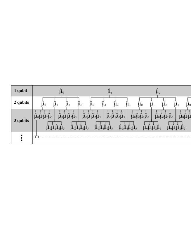
FIG. 1.: Tree diagram representing number and type of measurements necessary for tomography. For a single qubit, the measurements $\{\hat{\mu}_{0},\hat{\mu}_{1},\hat{\mu}_{2},\hat{\mu}_{3}\}$ suffice to reconstruct the state, e.g., measurements of the horizontal, vertical, diagonal and right-circular polarization components, (H,V,D,R). For two qubits, 16 double-coincidence measurements are necessary ($\{\hat{\mu}_{0}\hat{\mu}_{0},\hat{\mu}_{0}\hat{\mu}_{1}\ldots\hat{\mu}_{3}\hat{\mu}_{3}\}$), increasing to 64 three-coincidence measurements for three qubits ($\{\hat{\mu}_{0}\hat{\mu}_{0}\hat{\mu}_{0},\hat{\mu}_{0}\hat{\mu}_{0}\hat{\mu}_{1}\ldots\hat{\mu}_{3}\hat{\mu}_{3}\hat{\mu}_{3}\}$), and so on, as shown.

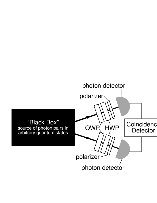
FIG. 2.: Schematic illustration of the experimental arrangement. “QWP” stands for quarter waveplate, “HWP” for half waveplate; the angles of both pairs of wave plates can be set independently giving the experimenter four degrees of freedom with which to set the projection state. In the experiment, the polarizers were realized using polarizing prisms, arranged to transmit vertically polarized light.

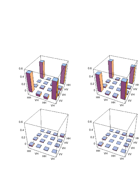
FIG. 3.: Graphical representation of the density matrix of a state as estimated by linear tomography (left) and by maximum likelihood tomography (right) from the experimental data given in the text. The upper plot is the real part of $\hat{\rho}$, the lower plot the imaginary part.

$\nu$	Mode 1	Mode 2	$h_{1}$	$q_{1}$	$h_{2}$	$q_{2}$
1	$|{\rm H}\rangle$	$|{\rm H}\rangle$	$45^{o}$	$0$	$45^{o}$	$0$
2	$|{\rm H}\rangle$	$|{\rm V}\rangle$	$45^{o}$	$0$	$0$	$0$
3	$|{\rm V}\rangle$	$|{\rm V}\rangle$	$0$	$0$	$0$	$0$
4	$|{\rm V}\rangle$	$|{\rm H}\rangle$	$0$	$0$	$45^{o}$	$0$
5	$|{\rm R}\rangle$	$|{\rm H}\rangle$	$22.5^{o}$	$0$	$45^{o}$	$0$
6	$|{\rm R}\rangle$	$|{\rm V}\rangle$	$22.5^{o}$	$0$	$0$	$0$
7	$|{\rm D}\rangle$	$|{\rm V}\rangle$	$22.5^{o}$	$45^{o}$	$0$	$0$
8	$|{\rm D}\rangle$	$|{\rm H}\rangle$	$22.5^{o}$	$45^{o}$	$45^{o}$	$0$
9	$|{\rm D}\rangle$	$|{\rm R}\rangle$	$22.5^{o}$	$45^{o}$	$22.5^{o}$	$0$
10	$|{\rm D}\rangle$	$|{\rm D}\rangle$	$22.5^{o}$	$45^{o}$	$22.5^{o}$	$45^{o}$
11	$|{\rm R}\rangle$	$|{\rm D}\rangle$	$22.5^{o}$	$0$	$22.5^{o}$	$45^{o}$
12	$|{\rm H}\rangle$	$|{\rm D}\rangle$	$45^{o}$	$0$	$22.5^{o}$	$45^{o}$
13	$|{\rm V}\rangle$	$|{\rm D}\rangle$	$0$	$0$	$22.5^{o}$	$45^{o}$
14	$|{\rm V}\rangle$	$|{\rm L}\rangle$	$0$	$0$	$22.5^{o}$	$90^{o}$
15	$|{\rm H}\rangle$	$|{\rm L}\rangle$	$45^{o}$	$0$	$22.5^{o}$	$90^{o}$
16	$|{\rm R}\rangle$	$|{\rm L}\rangle$	$22.5^{o}$	$0$	$22.5^{o}$	$90^{o}$
Table 1

TABLE 1: The tomographic analysis states used in our experiments. The number of coincidence counts measured in projections measurements provide a set of 16 data that allow the density matrix of the state of the two modes to be estimated. We have used the notation $|{\rm D}\rangle\equiv\left(|{\rm H}\rangle+|{\rm V}\rangle\right)/\sqrt{2}$, $|{\rm L}\rangle\equiv\left(|{\rm H}\rangle+i|{\rm V}\rangle\right)/\sqrt{2}$ and $|{\rm R}\rangle\equiv\left(|{\rm H}\rangle-i|{\rm V}\rangle\right)/\sqrt{2}$. Note that, when the measurement are taken in the order given by the table, only one waveplate angle had to be changed between each measurement.

REFERENCES

- [1] G. C. Stokes, Trans. Cambr. Phil. Soc. 9, 399 (1852).
- [2] U. Leonhardt, Measuring the quantum state of light (Cambridge University Press, 1997).
- [3] Z. Hradil, “Quantum-state estimation,” Phys. Rev. A55, R1561 (1997).
- [4] S. M. Tan, “An inverse problem approach to optical homodyne tomography,” J. Mod. Opt. 44, 2233 (1997).
- [5] K. Banaszek, G. M. D’Ariano, M. G. A. Paris and M. F. Sacchi, “Maximum-likelihood estimation of the density matrix,” Phys. Rev. A 61, 010304 (1999).
- [6] Z. Hradil, J. Summhammer, G. Badurek and H. Rauch, “Reconstruction of the spin state,” Phys. Rev. A 62, 014101 (2000).
- [7] J. Řeháček, Z. Hradil and M. Ježek, “Iterative algorithm for reconstruction of entangled states”, quant-ph/0009093 (submitted).
- [8] J.R. Ashburn, R.A. Cline, P.J.M. Vanderburgt, W.B. Westerveld and J.S. Risley, “Experimentally determined density-matrices for H(n=3) formed in -He collisions from 20 to 100 keV,” Phys. Rev. A 41, 2407-2421 (1990).
- [9] D. T. Smithey, M. Beck, M. G. Raymer and A. Faridani, “Measurement of the Wigner distribution and the density matrix of a light mode using optical homodyne tomography: Application to squeezed states and the vacuum,” Phys. Rev. Lett. 70, 1244 (1993).
- [10] G. Breitenbach, S. Schiller, J. Mlynek, “Measurement of the quantum states of squeezed light,” Nature 387, 471-475 (1997).
- [11] J. W. Wu, P. K. Lam, M. B. Gray and H.-A. Bachor, “Optical homodyne tomography of information carrying laser beams,” Optics Express 3, 154 (1998).
- [12] T.J. Dunn, I.A. Walmsley and S. Mukamel, “Experimental-determination of the quantum-mechanical state of a molecular vibrational-mode,” Phys. Rev. Lett. 74 884-887 (1995).
- [13] Experimental determination of the motional quantum state of a trapped atom D. Leibfried, D.M. Meekhof, B.E. King, C. Monroe, W.M. Itano and D.J. Wineland Phys. Rev. Lett. 77, 4281-4285 (1996); D. Leibfried, T. Pfau and C. Monroe, “Shadows and mirrors: Reconstructing quantum states of atom motion,” Physics Today 51(4), 22-28 (April 1998).
- [14] C. Kurtsiefer, T. Pfau, J. Mlynek, “Measurement of the Wigner function of an ensemble of helium atoms,” Nature 386, 150-153 (1997).
- [15] G. Klose, G. Smith and P. S. Jessen, “Measuring the Quantum State of a Large Angular Momentum,” submitted to Phys. Rev. Lett.; Los Alamos e-print archive quant-ph/0101017.
- [16] I.L. Chuang, N. Gershenfeld, M. Kubinec, “Experimental implementation of fast quantum searching,” Phys. Rev. Lett. 80 3408-3411 (1998).
- [17] S. L. Braunstein, C. M. Caves, R. Jozsa, N. Linden, S. Popescu and R. Schack, “Separability of very noisy mixed states and implications for NMR Quantum computing,” Phys. Rev. Lett. 83, 1054 (1999)
- [18] A. G. White, D. F. V. James, P. H. Eberhard and P. G. Kwiat, “Nonmaximally Entangled States: Production, Characterization, and Utilization,” Phys. Rev. Lett. 83, 3103 (1999).
- [19] A recent overview of many quantum computation technologies is given in Fort. d. Phys. 48 issue numbers 9-11 (2000) (S.L. Braunstein and H.K. Lo, eds.).
- [20] E. Hecht and A. Zajac Optics (Addision-Wesley, Reading MA, 1974) section 8.12.
- [21] E. Wolf, Il Nuovo Cimento 13, 1165 (1959); L. Mandel and E. Wolf Optical Coherence and Quantum Optics (Cambridge University Press, Cambridge, 1995), ch.6.
- [22] P. G. Kwiat, E. Waks, A. G. White, I. Appelbaum and P. H. Eberhard, “Ultrabright-source of polarization-entangled photons,” Phys. Rev. A 60, R773 (1999).
- [23] A. G. White, D. F. V. James, W. J. Munro and P. G. Kwiat, “Exploring Hilbert Space: accurate characterization of quantum information,” submitted to Science (2001).
- [24] A. Berglund, “Quantum coherence and control in one- and two-photon optical systems,” undergraduate thesis, Dartmouth College, June 2000; quant-ph/0010001.
- [25] W. H. Press, S. A. Teukolsky, W. T. Vetterling and B. P. Flannery, Numerical Recipes in Fortran 77: The Art of Scientific Computing (2nd ed., Cambridge University Press, Cambridge, 1992), section 10.5.
- [26] A. C. Melissinos, Experiments in Modern Physics (Academic Press, New York, 1966), §10.4, pp.467-479.
- [27] M. A. Nielsen and I. L. Chuang, Quantum Computation and Quantum Information (Cambridge University Press, Cambridge, 2000), ch.11.
- [28] L. I. Schiff, Quantum Mechanics (3rd Edition, McGraw-Hill, New York, 1968), eq.(31.8), p.246.
- [29] W. K. Wootters, “Entanglement of formation of an arbitrary state of two qubits,” Phys. Rev. Lett. 80, 2245 (1998); V. Coffman, J. Kundu, W. K. Wootters, “Distributed entanglement,” Phys. Rev. A 61, 052306 (2000).
- [30] B. M. Terhal, “Detecting Quantum Entanglement,” Quantum Physics preprint quant-ph/0101032.
- [31] The properties of the eigenvectors and eigenvalues of non-Hermitian matrices is discussed in P. M. Morse and H. Feshbach, Methods of Theoretical Physics (McGraw-Hill, New York, 1953), vol.I, p.884 et sequi.