Bohmian prediction about a two double-slit experiment and its disagreement with standard quantum mechanics

Abstract

The significance of proposals that can predict different results for standard and Bohmian quantum mechanics have been the subject of many discussions over the years. Here, we suggest a particular experiment (a two double-slit experiment) and a special detection process, that we call selective detection, to distinguish between the two theories. Using our suggested experiment, it is shown that the two theories predict different observable results at the individual level for a geometrically symmetric arrangement. However, their predictions are the same at the ensemble level. On the other hand, we have shown that at the statistical level, if we use our selective detection, then either the predictions of the two theories differ or where standard quantum mechanics is silent or vague, Bohmian quantum mechanics makes explicit predictions.

PACS number(s): 03.65.Bz

1 Introduction

According to the standard quantum mechanics (SQM), the complete description of a system of particles is provided by its wavefunction. The empirical predictions of SQM follow from a mathematical formalism which makes no use of the assumption that matter consists of particles pursuing definite tracks in space-time. It follows that the results of the experiments designed to test the predictions of the theory, do not permit us to infer any statement regarding the particle–not even its independent existence. But, in the Bohmian quantum mechanics (BQM), the additional element that is introduced apart from the wavefunction is the particle position, conceived in the classical sense as pursuing a definite continuous track in space-time [1-3]. The detailed predictions made by this causal interpretation explains how the results of quantum experiments come about but it is claimed that they are not tested by them. In fact when Bohm [1] presented his theory in 1952, experiments could be done with an almost continuous beam of particles, but not with individual particles. Thus, Bohm constructed his theory in such a fashion that it would be impossible to distinguish observable predictions of his theory from SQM. This can be seen from Bell’s comment about empirical equivalence of the two theories when he said:“It [the de Broglie-Bohm version of non-relativistic quantum mechanics] is experimentally equivalent to the usual version insofar as the latter is unambiguous”[4]. However, could it be that a certain class of phenomena might correspond to a well-posed problem in one theory but to none in the other? Or might the additional particles and definite trajectories of Bohm’s theory lead to a prediction of an observable where SQM would just have no definite prediction to make? To draw discrepancy from experiments involving the particle track, we have to argue in such a way that the observable predictions of the modified theory are in some way functions of the trajectory assumption. The question raised here is whether the de Broglie-Bohm particle law of motion can be made relevant to experiment. At first, it seems that definition of time spent by a particle within a classically forbidden barrier provides a good evidence for the preference of BQM. But, there are difficult technical questions, both theoretically and experimentally, that are still unsolved about this tunnelling times [3]. A recent work indicates that it is not practically feasible to use tunnelling effect to distinguish between the two theories [5].

On the other hand, Englert et al. [6] and Scully [7] have claimed that in some cases Bohm’s approach gives results that disagree with those obtained from SQM and, in consequence, with experiment. Again, at first Dewdney et al. [8] and then Hiley et al. [9] showed that the specific objections raised by Englert et al. and Scully cannot be sustained. Furthermore, Hiley believes that no experiment can decide between the standard interpretation and Bohm’s interpretation. However, Vigier [10], in his recent work, has given a brief list of new experiments which suggest that the U(1) invariant massless photon assumed properties of light within the standard interpretation, are too restrictive and that the O(3) invariant massive photon causal de Broglie-Bohm interpretation of quantum mechanics, is now supported by experiments. Furthermore, in some of the recent investigation, some feasible experiments have been suggested to distinguish between SQM and BQM [11, 12]. In one work, Ghose indicated that although BQM is equivalent to SQM when averages of dynamical variables are taken over a Gibbs ensemble of Bohmian trajectories, the equivalence breaks down for ensembles built over clearly separated short intervals of time in specially entangled two-bosonic particle systems [11]. Another one [12] is an extension of Ghose’s work to show disagreement between SQM and BQM in a two-particle system with an unentangled wavefunction, particularly at the statistical level. Further discussion of this subject can be found in [13-15]. In that experiment, to obtain a different interference pattern from SQM, we must deviate the source from its geometrically symmetric location.

In this investigation, we are offering a new thought experiment which can decide between SQM and BQM. Here, the deviation of the source from its geometrical symmetric location is not necessary and we have used a system consisting two correlated particles with an entangled wavefunction.

In the following section, we have introduced a two double-slit experimental set-up. In section 3, Bohm’s interpretation is used to find some observable results about our suggested experiment. Predictions of the standard interpretation and their comparison with Bohmian predictions is examined in section 4. In section 5, we have used selective detection and have compared SQM and BQM with our thought experiment at the ensemble level of particles, and we state our conclusion in section 6.

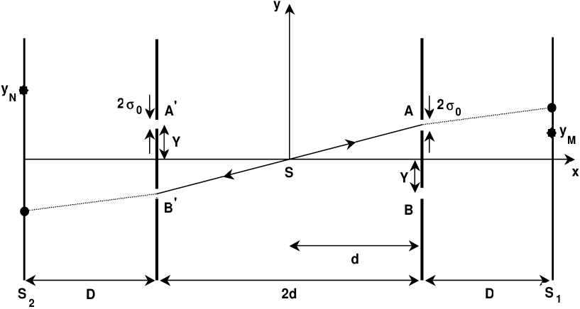
Figure 1: A two double-slit experiment configuration. Two identical particles with zero total momentum are emitted from the source $S$ and then they pass through slits $A$ and $B^{{}^{\prime}}$ or $B$ and $A^{{}^{\prime}}$. Finally, they are detected on $S_{1}$ and $S_{2}$ screens, simultaneously. It is necessary to note that dotted lines are not real trajectories.

2 Two double-slit experiment presentation

To distinguish between SQM and BQM we consider the following experimental set-up. A pair of identical non-relativistic particles with total momentum zero labelled by 1 and 2, originate from a point source S that is placed exactly in the middle of a two double-slit screens as shown in Fig. 1. We assume that the intensity of the beam is so low that during any individual experiment we have only a single pair of particles passing through the slits and the detectors have the opportunity to relate together for performing selective detection process. In addition, we assume that the detection screens $S_{1}$ and $S_{2}$ register only those pairs of particles that reach the two screens simultaneously. Thus, we are sure that the registration of single particles is eliminated from final interference pattern. The detection process at the screens $S_{1}$ and $S_{2}$ may be nontrivial but they play no causal role in the basic phenomenon of the interference of particles waves [2]. In the two-dimensional system of coordinates $(x,y)$ whose origin $S$ is shown, the center of slits lie at the points $(\pm d,\pm Y)$. The wave incident on the slits will be taken as a plane of the form

$$\psi_{in}(x_{1},y_{1};x_{2},y_{2};t)=ae^{i[k_{x}(x_{1}-x_{2})+k_{y}(y_{1}-y_{2})]}e^{-iEt/\hbar}$$ (1)

where $a$ is a constant and $E=E_{1}+E_{2}=\hbar^{2}(k_{x}^{2}+k_{y}^{2})/m$ is the total energy of the system of the two particles. The plane wave assumption comes from large distance between source $S$ and double-slit screens. To avoid the mathematical complexity of Fresnel diffraction at a sharp-edge slit, we suppose the slits have soft edges that generate waves having identical Gaussian profiles in the $y$-direction while the plane wave in the $x$-direction is unaffected [2]. The instant at which the packets are formed will be taken as our zero of time. Therefore, the four waves emerging from the slits $A$, $B$, $A^{{}^{\prime}}$ and $B^{{}^{\prime}}$ are initially

$$\psi_{A,B}(x,y)=a(2\pi\sigma_{0}^{2})^{-1/4}e^{-(\pm y-Y)^{2}/4\sigma_{0}^{2}}e^{i[k_{x}(x-d)+k_{y}(\pm y-Y)]}$$ (2)

$$\psi_{A^{{}^{\prime}},B^{{}^{\prime}}}(x,y)=a(2\pi\sigma_{0}^{2})^{-1/4}e^{-(\pm y+Y)^{2}/4\sigma_{0}^{2}}e^{i[-k_{x}(x+d)+k_{y}(\pm y+Y)]}$$ (3)

where $\sigma_{0}$ is the half-width of each slit. At time $t$ the general total wavefunction at a space point $(x,y)$ of our considered system for bosonic and fermionic particles is given by

$$\psi(x_{1},y_{1};x_{2},y_{2};t)=N[\psi_{A}(x_{1},y_{1},t)\psi_{B^{{}^{\prime}}}(x_{2},y_{2},t)\pm\psi_{A}(x_{2},y_{2},t)\psi_{B^{{}^{\prime}}}(x_{1},y_{1},t)$$

$$+\psi_{B}(x_{1},y_{1},t)\psi_{A^{{}^{\prime}}}(x_{2},y_{2},t)\pm\psi_{B}(x_{2},y_{2},t)\psi_{A^{{}^{\prime}}}(x_{1},y_{1},t)]$$ (4)

with

$$\psi_{A,B}(x,y,t)=a(2\pi\sigma_{t}^{2})^{-1/4}e^{-(\pm y-Y-u_{y}t)^{2}/4\sigma_{0}\sigma_{t}}e^{i[k_{x}(x-d)+k_{y}(\pm y-Y-u_{y}t/2)-E_{x}t/\hbar]}$$ (5)

$$\psi_{A^{{}^{\prime}},B^{{}^{\prime}}}(x,y,t)=a(2\pi\sigma_{t}^{2})^{-1/4}e^{-(\pm y-Y-u_{y}t)^{2}/4\sigma_{0}\sigma_{t}}e^{i[-k_{x}(x+d)+k_{y}(\pm y-Y-u_{y}t/2)-E_{x}t/\hbar]}$$ (6)

where $N$ is a reparametrization constant that its value is unimportant in this paper and

$$\sigma_{t}=\sigma_{0}(1+\frac{i\hbar t}{2m\sigma_{0}^{2}})$$ (7)

$$u_{y}=\frac{\hbar k_{y}}{m}$$

$$E_{x}=\frac{1}{2}mu_{x}^{2}$$ (8)

where $u_{x}$ and $u_{y}$, according to BQM, are initial group velocities corresponding to each particle in the $x$- and $y$-directions, respectively. In addition, the upper and lower sings in the total wavefunction refer to symmetric and anti-symmetric wavefunction under exchange of particle 1 to particle 2, corresponding to bosonic and fermionic property, while in the equations (5) and (6) they refer to upper and lower slits, respectively. In the next section, we have used BQM to drive some results of this experiment.

3 Bohmian predictions about the suggested experiment

In BQM, the complete description of a system is given by specifying the position of the particles in addition to their wavefunction which has the role of guiding the particles according to following guidance condition for $n$ particles, with masses $m_{1},m_{2},...,m_{n}$

$$\overrightarrow{\dot{x}_{i}}(\overrightarrow{x},t)=\frac{1}{m_{i}}\overrightarrow{\nabla_{i}}S(\overrightarrow{x},t)=\frac{\hbar}{m_{i}}Im\left(\frac{\overrightarrow{\nabla_{i}}\psi(\overrightarrow{x},t)}{\psi(\overrightarrow{x},t)}\right)$$ (9)

where $\overrightarrow{x}=(\overrightarrow{x_{1}},\overrightarrow{x_{2}},...,\overrightarrow{x_{n}})$ and

$$\psi(\overrightarrow{x_{1}},\overrightarrow{x_{2}},...,\overrightarrow{x_{n}};t)=R(\overrightarrow{x_{1}},\overrightarrow{x_{2}},...,\overrightarrow{x_{n}};t)e^{iS(\overrightarrow{x_{1}},\overrightarrow{x_{2}},...,\overrightarrow{x_{n}};t)/\hbar}$$ (10)

is a solution of Schr$\ddot{o}$dinger’s wave equation. Thus, instead of SQM with indistinguishable particles, in BQM the path of particles or their individual histories distinguishes them and each one of them can be studied separately [2]. In addition, Belousek [16] in his recent work, concluded that the problem of Bohmian mechanical particles being statistically (in)distinguishable is a matter of theory choice underdetermined by logic and experiment, and that such particles are in any case physically distinguishable. For our considered experiment, the speed of the particles 1 and 2 in the $y$-direction is given , respectively, by

$$\dot{y}_{1}(x_{1},y_{1};x_{2},y_{2};t)=\frac{\hbar}{m}Im\frac{\partial_{y_{1}}\psi(x_{1},y_{1};x_{2},y_{2};t)}{\psi(x_{1},y_{1};x_{2},y_{2};t)}$$ (11)

$$\dot{y}_{2}(x_{1},y_{1};x_{2},y_{2};t)=\frac{\hbar}{m}Im\frac{\partial_{y_{2}}\psi(x_{1},y_{1};x_{2},y_{2};t)}{\psi(x_{1},y_{1};x_{2},y_{2};t)}.$$ (12)

With the replacement of $\psi(x_{1},y_{1};x_{2},y_{2};t)$ from (4), (5) and (6), we have

$$\dot{y}_{1} = N\frac{\hbar}{m}Im\{\frac{1}{\psi}[[-2(y_{1}-Y-u_{y}t)/4\sigma_{0}\sigma_{t}+ik_{y}]\psi_{A_{1}}\psi_{B^{{}^{\prime}}_{2}}$$ (13)

$$\pm [-2(y_{1}+Y+u_{y}t)/4\sigma_{0}\sigma_{t}-ik_{y}]\psi_{A_{2}}\psi_{B^{{}^{\prime}}_{1}}$$ (14)

$$+ [-2(y_{1}+Y+u_{y}t)/4\sigma_{0}\sigma_{t}-ik_{y}]\psi_{B_{1}}\psi_{A^{{}^{\prime}}_{2}}$$ (15)

$$\pm [-2(y_{1}-Y-u_{y}t)/4\sigma_{0}\sigma_{t}+ik_{y}]\psi_{B_{2}}\psi_{A^{{}^{\prime}}_{1}}]\}$$ (16)

$$\dot{y}_{2} = N\frac{\hbar}{m}Im\{\frac{1}{\psi}[[-2(y_{2}+Y+u_{y}t)/4\sigma_{0}\sigma_{t}-ik_{y}]\psi_{A_{1}}\psi_{B^{{}^{\prime}}_{2}}$$ (17)

$$\pm [-2(y_{2}-Y-u_{y}t)/4\sigma_{0}\sigma_{t}+ik_{y}]\psi_{A_{2}}\psi_{B^{{}^{\prime}}_{1}}$$ (18)

$$+ [-2(y_{2}-Y-u_{y}t)/4\sigma_{0}\sigma_{t}+ik_{y}]\psi_{B_{1}}\psi_{A^{{}^{\prime}}_{2}}$$ (19)

$$\pm [-2(y_{2}+Y+u_{y}t)/4\sigma_{0}\sigma_{t}-ik_{y}]\psi_{B_{2}}\psi_{A^{{}^{\prime}}_{1}}]\}$$ (20)

where, for example, the short notation $\psi_{A}(x_{1},y_{1},t)=\psi_{A_{1}}$ is used. Furthermore, from (5) and (6) it is clear that

$$\psi_{A}(x_{1},y_{1},t)=\psi_{B}(x_{1},-y_{1},t)$$ (21)

$$\psi_{A}(x_{2},y_{2},t)=\psi_{B}(x_{2},-y_{2},t)$$ (22)

$$\psi_{B^{{}^{\prime}}}(x_{1},y_{1},t)=\psi_{A^{{}^{\prime}}}(x_{1},-y_{1},t)$$ (23)

$$\psi_{B^{{}^{\prime}}}(x_{2},y_{2},t)=\psi_{A^{{}^{\prime}}}(x_{2},-y_{2},t)$$ (24)

which indicates the reflection symmetry of $\psi(x_{1},y_{1};x_{2},y_{2};t)$ with respect to the $x$–axis. Utilizing this symmetry in (13) and (14), we can see that

$$\dot{y}_{1}(x_{1},y_{1};x_{2},y_{2};t)=-\dot{y}_{1}(x_{1},-y_{1};x_{2},-y_{2};t)$$ (25)

$$\dot{y}_{2}(x_{1},y_{1};x_{2},y_{2};t)=-\dot{y}_{2}(x_{1},-y_{1};x_{2},-y_{2};t)$$ (26)

which are valid for both bosonic and fermionic particles. Relations (16) show that if $y_{1}(t)=y_{2}(t)=0$, then the speed of each particles in the $y$-direction is zero along the symmetry axis $x$. This means that none of the particles can cross the $x$-axis nor are they tangent to it, provided both of them are simultaneously on this axis. Similar conclusions can be found in some other works [for example, 8, 9, 11-13]. It can be seen that there is the same symmetry of the velocity about the $x$-axis as for an ordinary double-slit experiment [2].

If we consider $y=(y_{1}+y_{2})/2$ to be the vertical coordinate of the center of mass of the two particles, then we can write

$$\dot{y} = (\dot{y}_{1}+\dot{y}_{2})/2$$ (27)

$$= -N\frac{\hbar}{2m}Im\{{\frac{1}{\psi}(\frac{y_{1}+y_{2}}{2\sigma_{0}\sigma_{t}})(\psi_{A_{1}}\psi_{B^{{}^{\prime}}_{1}}\pm\psi_{A_{2}}\psi_{B^{{}^{\prime}}_{1}}+\psi_{B_{1}}\psi_{A^{{}^{\prime}}_{2}}\pm\psi_{B_{2}}\psi_{A^{{}^{\prime}}_{1}})}\}$$ (28)

$$= \frac{(\hbar/2m\sigma_{0}^{2})^{2}}{1+(\hbar/2m\sigma_{0}^{2})^{2}t^{2}}yt.$$ (29)

Solving the equation of motion (17), we obtain the path of the $y$-coordinate of the center of mass

$$y=y_{0}\sqrt{1+(\hbar/2m\sigma_{0}^{2})^{2}t^{2}}.$$ (30)

If at $t=0$ the center of mass of the two particles is exactly on the $x$-axis, then $y_{0}=0$, and the center of mass of the particles will always remain on the $x$-axis. Thus, according to BQM, the two particles will be detected at points symmetric with respect to the $x$-axis, as shown in Fig. 1.

It seems that calculation of quantum potential can give us another perspective of this experiment. As we know, to see the connection between the wave and particle, the Schr$\ddot{o}$dinger equation can be rewritten in the form of a generalized Hamilton-jacobi equation that has the form of the classical equation, apart from the extra term

$$Q(\overrightarrow{x},t)=-\frac{\hbar^{2}}{2m}\frac{\nabla^{2}R(\overrightarrow{x},t)}{R(\overrightarrow{x},t)}$$ (31)

where function Q has been called the quantum potential [2]. But, it is clear that the calculation and analysis of Q, by using our total wavefunction (4), is not very simple. On the other hand, we can use the form of Newton’s second law, in which the particle is subject to a quantum force $(-\overrightarrow{\nabla}Q)$ in addition to the classical force $(-\overrightarrow{\nabla}V)$ [2], namely

$$\overrightarrow{F}=-\overrightarrow{\nabla}(Q+V).$$ (32)

Now, if we utilize the equation of motion of the center of mass $y$-coordinate (18) and the equation (20), we shall obtain the quantum potential for the center of mass motion $(Q_{cm})$. Thus, we can write

$$-\frac{\partial Q}{\partial x}=m\ddot{x}=0$$ (33)

$$-\frac{\partial Q}{\partial y}=m\ddot{y}=\frac{my_{0}(\hbar/2m\sigma_{0}^{2})^{2}}{(1+(\hbar t/2m\sigma_{0}^{2})^{2})^{3/2}}=\frac{my_{0}^{4}}{y^{3}}(\frac{\hbar}{2m\sigma_{0}^{2}})^{2}$$ (34)

where the result of equation (21) is clearly due to motion of plane wave in the $x$-direction. In addition, we assume that $\nabla V=0$ in our experiment. Thus, our effective quantum potential is only a function of $y$-variable and it has the form

$$Q=\frac{my_{0}^{4}}{2y^{2}}(\frac{\hbar}{2m\sigma_{0}^{2}})^{2}=\frac{1}{2}my_{0}^{2}\frac{\hbar/2m\sigma_{0}^{2})^{2}}{1+(\hbar t/2m\sigma_{0}^{2})^{2}}.$$ (35)

If $y_{0}=0$, the quantum potential for the center of mass of the two particles is zero at all times and it remains on the $x$-axis. However, if $y_{0}\neq 0$, then the center of mass cannot touch or cross the $x$-axis. These conclusions are consistent with our earlier result (eq. (18)).

4 SQM forecast and its comparison with BQM

So far, we have been studying the results obtained from BQM at the individual level. But it is well known from SQM that the probability of simultaneous detection of two particles at $y_{M}$ and $y_{N}$, at the screen $S_{1}$ and $S_{2}$ is equal to

$$P_{12}(y_{M},y_{N})=\int_{y_{M}}^{y_{M}+\triangle}dy_{1}\int_{y_{N}}^{y_{N}+\triangle}dy_{2}|\psi(x_{1},y_{1};x_{2},y_{2};t)|^{2}.$$ (36)

The parameter $\Delta$, which is taken to be small, is a measure of the size of the detectors. It is clear that the probabilistic prediction of SQM is in disagreement with the symmetrical prediction of BQM, because SQM predicts that probability of asymmetrical detection at the individual level of pair of particles can be different from zero, in opposition to BQM’s symmetrical predictions. In addition, based on SQM’s prediction, the probability of finding two particles at one side of the $x$-axis can be nonzero while we showed that BQM’s prediction forbids such events in our experiment. In other words, its probability must be exactly zero. Thus, if we provide necessary arrangements to perform this experiment, we must abandon one of the two theories or even both as a complete description of the universe.

Now the question arises as to whether this difference persists if we deal with an ensemble of pair of particles? To answer this question, we consider an ensemble of pair of particles that have arrived at the detection screens $S_{1}$ and $S_{2}$ at different times $t_{i}$. It is well known that, in order to ensure the compatibility between SQM and BQM for ensemble of particles, Bohm added a further postulate to his three basic and consistent postulates [1, 2]. Based on this further postulate, the probability that a particle in the ensemble lies between $\overrightarrow{x}$ and $\overrightarrow{x}+d\overrightarrow{x}$ at time $t$ is given by

$$P(\overrightarrow{x},t)=R^{2}(\overrightarrow{x},t).$$ (37)

Thus, using BQM, the probability of simultaneous detection for all pairs of particles of the ensemble arriving at the two screens at different instant of time $t_{i}$, with $y_{0}=0$, is

$$P_{12}=\lim_{N\rightarrow\infty}\sum_{i=1}^{N}R^{2}(y_{1}(t_{i}),-y_{1}(t_{i}),t_{i})\equiv\int^{+\infty}_{-\infty}dy_{1}\int^{+\infty}_{-\infty}dy_{2}|\psi(y_{1},y_{2},t)|^{2}=1$$ (38)

where every term in the sum shows only one pair arriving on the screens $S_{1}$ and $S_{2}$ at the point $(y_{1}(t_{i}),-y_{1}(t_{i}))$ and time $t_{i}$, weighted by the corresponding density $R^{2}$. If all times of $t_{i}$ are taken to be $t$, then the summation on $i$ can be changed to an integral over all paths that cross the screens $S_{1}$ and $S_{2}$ at that time. Now, we can consider the joint probability of two points $y_{M}$ and $y_{N}$ on the two screens at time $t$ that are not symmetric about the $x$-axis, but we know that they are not detected simultaneously. Then, one can obtain the probability of detecting two particles at two arbitrary points $y_{M}$ and $y_{N}$

$$P_{12}(y_{M},y_{N})=\int_{y_{M}}^{y_{M}+\Delta}dy_{1}\int_{y_{N}}^{y_{N}+\Delta}dy_{2}|\psi(y_{1},y_{2},t)|^{2}$$ (39)

which is similar to the prediction of SQM (eq. (24)) but obtained in a Bohmian way [11]. Thus, it appears that for a geometrically symmetric arrangement, the possibility of distinguishing the two theories at the statistical level is impossible, as was expected [1-3, 9, 17].

5 Selective detection and comparison of SQM with BQM at the statistical level

In the previous section, we have shown that SQM and BQM have different predictions for our suggested experiment, at the individual level. Since SQM talks about individual events in probabilistic terms, the existence of different predictions by the two theories at the individual level is not a strange result. On the other hand, we have seen that the two theories, for a geometrically symmetric arrangement, are consistent at the ensemble level. Here, one can ask whether the individual level is the only area to distinguish between the two theories and whether the disagreement between them cannot appear at the ensemble level. In this section, we answer this question in negative, and we shall provide conditions under which SQM can be interpreted as a vague theory at the ensemble level.

5.1 The case where $y_{0}$ is exactly zero

We have seen that the assumption of $y_{0}=0$ is not in contradiction with the statistically results of SQM and, in consequence, with experiment. Thus, we can assume that initially each particle in the source is statistically distributed according to the absolute square of the wavefunction, but, this distribution is completely symmetric so that the $y$-coordinate of the center of mass is on the $x$-axis. If we can prepare such a special source with two correlated particles, we can try to do our experiment in the following fashion: particles emitted from the source $S$ into the right hand side of the experimental set-up can pass through slits $A$ or $B$. Since we have assumed that the total momentum of the pair of particles is zero, if one of the particles goes through the slit $A$ for instance, the other particle must go through the slit $B^{{}^{\prime}}$ on the left hand side of the experimental set-up. Based on BQM and using equation (16), we infer that the particle passing through the slit $A$ must be detected on the upper half plane of the $x$-axis on the screen $S_{1}$. The same thing must occur for the other particle that passes through $B^{{}^{\prime}}$, but in the lower half plane of the $x$-axis on the $S_{2}$ screen. Using this prediction, we assume that only those particles arriving at $S_{2}$ are recorded for which there is a simultaneous detection of the other particle at the upper side on $S_{1}$. We called this special detection, in which some of the selected particles are recorded, a selective detection. Thus, based on the prediction power of BQM, we will record two particles symmetric with respect to the $x$-axis, for each emitted pairs of particles. If we wait to record an ensemble of particles, we will see an interference pattern of particles on the lower half plane of the $S_{2}$ screen. On the other hand, based on SQM, the probability of finding a particle at any point on the $S_{2}$ screen, even at the upper side, is nonzero and there is no compulsion to detect pairs of particles symmetrically on the two sides of the $x$-axis, as it can be seen from equation (24) and is depicted in Fig. 1. Therefore, if we accept that SQM is still efficient and unambiguous for the selective detection, the interference pattern will be seen on the whole screen $S_{2}$, particularly at the upper side of it, at the ensemble level. Consequently, we shall have observable results to distinguish the two theories, SQM and BQM.

5.2 The case where $y_{0}$ is statistically distributed

One can argue that $y_{0}$ cannot have a well-defined position and it must be distributed according to Born’s principle. However, we will show that this objection cannot alter our obtained results. Assume that, $\langle y_{0}\rangle=0$ but $\triangle y_{0}\neq 0$. If we provide conditions in which $\triangle y_{0}$ is very small and $\hbar t/2m\sigma_{0}^{2}\sim 1$, we can still detect particles symmetrically with respect to the $x$-axis, with a good approximation. To obtain symmetrical detection about the $x$-axis with reasonable approximation, the center of mass variation from the $x$-axis must be smaller than the distance between any two neighboring maxima, that is

$$y\ll\frac{\lambda D}{2Y}\simeq\frac{\pi\hbar t}{Ym}$$ (40)

where $\lambda$ is the de Broglie wavelength. For conditions $\hbar t/2m\sigma_{0}^{2}\sim 1$, $Y\sim\sigma_{0}$ and using equation (18), one can obtain

$$y_{0}\ll\frac{\pi\hbar t}{Ym}\sim\sigma_{0}.$$ (41)

Therefore, if we use a source with $\triangle y_{0}\ll\sigma_{0}$, we shall obtain $y\simeq y_{0}\ll\sigma_{0}$ for each individual observation, and our symmetrical detection can be maintained with a good approximation. It is evident that, if one considers $\triangle y_{0}\sim\sigma_{0}$, as was done in [15], the incompatibility between the two theories will be disappeared. But, we believe that, instead of the usual one-particle two-slit experiment with $\triangle y_{0}\sim\sigma_{0}$, our correlated two-particle system provides a new situation in which we can adjust $y_{0}$ independent of $\sigma_{0}$, so that

$$y_{0}=\frac{1}{2}(y_{1}+y_{2})_{t=0}\ll\sigma_{0}.$$ (42)

Although it is obvious that $(\triangle y_{1})_{t=0}=(\triangle y_{2})_{t=0}\sim\sigma_{0}$, but position correlation between the two entangled particles cause that they always satisfy equation (30). Furthermore, if it is assumed that $y_{0}$ is statistically distributed, another problem can be raised, which is mentioned by Marchildon [15]. We have shown that, if both particles are simultaneously on the $x$-axis, both velocities in the $y$-direction vanish, and neither particle could cross or be tangent to the $x$-axis. However, under $\triangle y_{0}\neq 0$ condition, pairs of particles cannot be simultaneously on the $x$-axis and we have not the aforementioned constraint on the motion of particles (relations (16)). However, using our selective detection, we can still obtain our last result, because the center of mass of the two particles are on the $x$-axis with reasonable approximation. It is clear that, under such a condition, one cannot claim that the particle detected at the upper (lower) side must have passed through upper (lower) slit, in spite of $y_{0}=0$ condition. To confirm these results, it is worth noting that, Durr et al. [17] argue that the selective detection can alter the statistical predictions of the two theories:“note that by selectively forgetting results we can dramatically alter the statistics of those that we have not forgotten. This is a striking illustration of the way in which Bohmian mechanics does not merely agree with the quantum formalism, but, eliminating ambiguities, clarifies, and sharpens it.”. Elsewhere [13], we have utilized another kind of selective detection by which we could alter statistical prediction of SQM, using BQM for an interference device that contains two unentangled particles.

6 Conclusion

In this investigation, we have suggested an experiment to distinguish between SQM and BQM. In fact, we believe that some particular experiments that for one reason or another have not yet been performed can decide between them. Thus, it has been shown that a two double-slit experiment set-up, along with a source of two identical non-relativistic particles with total momentum of zero, emitted at suitable time intervals, has the following characteristics:
1) The suggested experiment will yield different observable predictions for SQM and BQM, at the individual level.
2) The two theories yield the same interference pattern at the ensemble level without using a selective detection, as is expected.
3) Since in BQM the particles are distinguishable and their past history are known, using selective detection, it has been shown that either the two theories will predict different results at the statistical level, or that BQM has more predictive power than SQM. It is shown that selective detection can be considered as a tool for arriving to a new realm in which trajectory interpretation is sharply formulated, while the standard interpretation is ambiguous and silent even at the ensemble level.

Therefore, it seems possible to distinguish between the two theories and to see whether BQM is a worthy successor to SQM.

References

- [1] D. Bohm, Part I, Phys. Rev. 85 166 (1952); Part II, 85 180 (1952).
- [2] P.R. Holland, The Quantum Theory of Motion, Cambridge University Press, Cambridge, 1993.
- [3] J.T. Cushing, Quantum Mechanics: Historical Contingency and the Copenhagen Hegemony, The University of Chicago Press, Ltd., London, 1994.
- [4] J.S. Bell, Speakable and Unspeakable in Quantum Mechanics, Cambridge University Press, Cambridge, 1987.
- [5] M. Abolhasani and M. Golshani, Phys. Rev. A 62 12106 (2000).
- [6] B.G. Englert, M.O. Scully, G. Sussman and H. Walther, Z. Naturf. 47a 1175 (1992).
- [7] M.O. Scully, Phys. Scripta, T76 41 (1998).
- [8] C. Dewdney, L. Hardy and E.J. Squires, Phys. Lett. A 184 6 (1993).
- [9] B.J. Hiley, R.E. Callaghan and O.J.E. Maroney, quant-ph/0010020.
- [10] J.P. Vigier, Phys. Lett. A 270 221 (2000).
- [11] P. Ghose, quant–ph/0001024 and quant-ph/0003037.
- [12] M. Golshani and O. Akhavan, quant-ph/0009040.
- [13] M. Golshani and O. Akhavan, quant-ph/0103100.
- [14] P. Ghose, quant-ph/0102131.
- [15] L. Marchildon, quant-ph/0101132.
- [16] D.W. Belousek, Found. Phys. 30 153 (2000).
- [17] D. Durr, S. Goldstein and N. Zanghi, J. Stat. Phys. 67 843 (1992).