Experiment can decide between
standard and Bohmian quantum mechanics

Abstract

In this investigation, we have considered two thought experiments to make a comparison between predictions of the standard and the Bohmian quantum mechanics. Concerning this, a two-particle system has been studied at two various situations of the entangled and the unentangled states. In the first experiment, the two theories can predict different results at the individual level, while their statistical results are the same. In the other experiment, not only they are in disagreement at the individual level, but their equivalence at the statistical level also breaks down, if one uses selective detection. Furthermore, we discuss about some objections that can be raised against the results of the two suggested experiments.

PACS number: 03.65.Bz
Keywords: Bohmian quantum mechanics, Thought experiment, Entanglement, Selective detection, Inconsistent prediction

1 Introduction

The statistical interpretation of the wave function of the standard quantum mechanics (SQM) is consistent with all performed experiments. An interference pattern on a screen is built up by a series of apparently random events, and the wave function correctly predicts where the particle is most likely to land in an ensemble of trials. Instead, one may take the view that the characteristic distribution of spots on a screen which build up an interference pattern is an evidence that the wave function has a more potent physical role. If one attempts to understand the experimental results as the outcome of a causally connected series of individual process, then one is free to inquire about further significance of the wave function and to introduce other concepts in addition to the wave function. Bohm [1], in 1952, showed that an individual physical system comprises a wave propagating in space-time together with a point particle which moves continuously under the guidence of the wave [1-4]. He applied his theory to a range of examples drawn from non-relativistic quantum mechanics and speculated on the possible alternations in the particle and field laws of motion such that the predictions of the modified theory continue to agree with those of SQM where this is tested, but it could disagree in as yet unexplored domains [3]. For instance, when Bohm presented his theory in 1952, experiments could be done with an almost continuous beam of particles. Thus, it was impossible to discriminate between the standard and the Bohmian quantum mechanics (BQM) at the individual level. However, the two theories can be discriminated at this level, because SQM is a probabilistic theory while BQM is a precisely defined and deterministic theory.

In recent years, the significance of proposals that can predict different results for SQM and BQM have been the subject of many discussions [for example, 5-17]. At first, it seems that definition of time spent by a particle within a classically forbidden barrier provides a good evidence for the preference of BQM. But, there are difficult technical questions, both theoretically and experimentally, that are still unsolved about these tunneling times [4,5]. On the other hand, Englert et al. [6] and Scully [7] have claimed that in some cases Bohm’s approach gives results that disagree with those obtained from SQM and, in consequence, with experiment. Concerning this, at first Dewdney et al. [8] and then Hiley et al. [9] showed that the specific objections raised by Englert and Scully cannot be sustained. Furthermore, Hiley et al. [9] believe that no experiment can decide between the standard interpretation and Bohm’s interpretation. However, Vigier [10], in his recent work, has given a brief list of new experiments which suggest that the U(1) invariant massless photon assumed properties of light within the standard interpretation, are too restrictive and that the O(3) invariant massive photon causal de Broglie-Bohm interpretation of quantum mechanics, is now supported by experiments. In addition, Leggett [11] considered some thought experiments involving macrosystems which can predict different results for SQM and BQM. Furthermore, in some of the recent works, feasible thought experiments have been suggested to distinguish between SQM and BQM [12,13,17]. In one of the works, Ghose [12] indicated that although BQM is equivalent to SQM when the averages of dynamical variables are taken over a Gibbs ensemble of Bohmian trajectories, the equivalence breaks down for ensembles built over clearly separated short intervals of time in special entangled two-bosonic particle systems. In another work [13], we have shown incompatibility between SQM and BQM at the individual and ensemble levels, using a two-slit device whose source emits two uncorrelated identical particles. However, Marchildon [14,15] has tried to show that there is no reason to expect discrepancies between BQM and SQM in the context of the two-particle interference devices. Ghose [16] believes that Marchildon’s arguments against his work are untenable and that his basic conclusion stands. In addition, we have shown elsewhere [17] that the incompatibility between SQM and BQM can also appeare in a new more feasible experiment at the individual level and that the statistical disagreement is also valid if we use our selective detection. It should be noted that, the role of selective detection in altering the statistics of predictions is explained by Durr et al. [18].

In this work, in parallel to the works [12,13], we have studied the entangled and the unentangled wave functions that can be imputed to a two-particle interference device, using a Gaussian wave function as a real representation. Then, SQM and BQM predictions are compared at both the individual and the statistical level. We also discuss about some objections that can be raised.

2 Description of two-particle double-slit experiment

Consider the famous double-slit experiment. Instead of the usual one-particle emitting source, one can consider a special point source $S_{1}$, so that a pair of identical non-relativistic particles originate simultaneously from it. We assume that, the intensity of the beam is so low that at a time we have only a single pair of particles passing through the slits and the detection screen $S_{2}$ registers only those pairs of particles that reach it simultaneously, so that the interference effects of single particles will be eliminated. Furthermore, it is assumed that the detection process has no causal role in the phenomenon of interference [3]. In the two-dimensional coordinate system, the centers of the two slits are located at $(0,\pm Y)$.

Concerning the assumed source, we can have two alternatives:
1. The wave function of the two emitted particles are so entangled that if one particle passes from the upper (lower) slit, the other particle must go through lower (upper) slit. In other words, the total momentum and the center of mass of the two particles in the $y$-direction is zero at the source, that is, $p_{1y}-p_{2y}=0$ and $y_{1}+y_{2}=0$.
2. The wave function of the two emitted particles have no correlation and they are unentangled. In other words, the emission of each particle is done freely and two particles can be considered independently.
In the following, we shall study each one of the two alternatives, separately, and apply them, using SQM. Then, in the next section, the Bohmian predictions have been compared with those of SQM.

2.1 Entangled wave function

We take the wave incident on the double-slit screen to be a plane wave of the form

$$\psi_{in}(x_{1},y_{1};x_{2},y_{2};t)=ae^{i[k_{x}(x_{1}+x_{2})+k_{y}(y_{1}-y_{2})]}e^{-iEt/\hbar},$$ (1)

where $a$ is a constant and $E=E_{1}+E_{2}=\hbar^{2}(k_{x}^{2}+k_{y}^{2})/m$ is the total energy of the system of the two identical particles. The parameter $m$ is the mass of each particle and $k_{i}$ is the wave number of particle in the $i$-direction. For mathematical simplicity, we avoid slits with sharp edges which produce the mathematical complexity of Fresnel diffraction, i.e., we assume that the slits have soft edges, so that the Gaussian wave packets are produced along the $y$-direction, and that the plane wave along the $x$-axis remain unchanged [3]. We take the time of the formation of the Gaussian wave to be $t=0$. Then, the emerging wave packets from the slits $A$ and $B$ are respectively

$$\psi_{A}(x,y)=a(2\pi\sigma_{0}^{2})^{-1/4}e^{-(y-Y)^{2}/4\sigma_{0}^{2}}e^{i[k_{x}x+k_{y}(y-Y)]},$$ (2)

$$\psi_{B}(x,y)=a(2\pi\sigma_{0}^{2})^{-1/4}e^{-(y+Y)^{2}/4\sigma_{0}^{2}}e^{i[k_{x}x-k_{y}(y+Y)]},$$ (3)

where $\sigma_{0}$ is the half-width of each slit.

Now, for this two-particle system, the total wave function at the detection screen $S_{2}$, at time $t$, can be written as

$$\psi(x_{1},y_{1};x_{2},y_{2};t)=N[\psi_{A}(x_{1},y_{1},t)\psi_{B}(x_{2},y_{2},t)\pm\psi_{A}(x_{2},y_{2},t)\psi_{B}(x_{1},y_{1},t)],$$ (4)

where $N$ is a normalization constant which is unimportant here, and

$$\psi_{A}(x,y,t)=a(2\pi\sigma_{t}^{2})^{-1/4}e^{-(y-Y-u_{y}t)^{2}/4\sigma_{0}\sigma_{t}}e^{i[k_{x}x+k_{y}(y-Y-u_{y}t/2)-E_{x}t/\hbar]},$$ (5)

$$\psi_{B}(x,y,t)=a(2\pi\sigma_{t}^{2})^{-1/4}e^{-(y+Y+u_{y}t)^{2}/4\sigma_{0}\sigma_{t}}e^{i[k_{x}x-k_{y}(y+Y+u_{y}t/2)-E_{x}t/\hbar]},$$ (6)

where

$$\sigma_{t}=\sigma_{0}(1+\frac{i\hbar t}{2m\sigma_{0}^{2}}),$$ (7)

and

$$u_{y}=\frac{\hbar k_{y}}{m},$$ (8)

$$E_{x}=\frac{1}{2}mu_{x}^{2}.$$ (9)

Note that, the upper and lower signs in the total entangled wave function (4) are due to symmetric and anti-symmetric wave function under the exchange of particles 1 and 2, corresponding to bosonic and fermionic property, respectively.

2.2 Unentangled wave function

In this case, the incident plane wave can be considered to be

$$\tilde{\psi}_{in}(x_{1},y_{1};x_{2},y_{2};t)=ae^{i[k_{x}(x_{1}+x_{2})+k_{y}(\pm y_{1}\pm y_{2})]}e^{-iEt/\hbar},$$ (10)

where it has four cases corresponding to each sign. Now, for this two-particle system, the total wave function at time $t$ can be written as

$$\tilde{\psi}(x_{1},y_{1};x_{2},y_{2};t)=$$ (14)

$$\widetilde{N}[\psi_{A}(x_{1},y_{1},t)\psi_{B}(x_{2},y_{2},t)+\psi_{A}(x_{2},y_{2},t)\psi_{B}(x_{1},y_{1},t)$$

$$+\psi_{A}(x_{1},y_{1},t)\psi_{A}(x_{2},y_{2},t)+\psi_{B}(x_{1},y_{1},t)\psi_{B}(x_{2},y_{2},t)]$$

$$=\widetilde{N}[\psi_{A}(x_{1},y_{1},t)+\psi_{B}(x_{1},y_{1},t)][\psi_{A}(x_{2},y_{2},t)+\psi_{B}(x_{2},y_{2},t)],$$

where $\widetilde{N}$ is another normalization constant.

2.3 SQM’s prediction

Based on SQM, the wave function can be associated with an individual physical system. It provides the most complete description of the system that is, in principle, possible. The nature of description is statistical, and concerns the probabilities of the outcomes of all conceivable measurements that may be performed on the system. It is well known from SQM that, the probability of simultaneous detection of the particles at $y_{M}$ and $y_{N}$, at the screen $S_{2}$, located at $x_{1}=x_{2}=D$ and $t=D/u_{x}$, is equal to

$$P_{12}(y_{M},y_{N},t)=\int_{y_{M}}^{y_{M}+\triangle}dy_{1}\int_{y_{N}}^{y_{N}+\triangle}dy_{2}|\psi(x_{1},y_{1};x_{2},y_{2};t)|^{2}.$$ (15)

The parameter $\Delta$, which is taken to be small, is a measure of the size of the detectors. We shall compare this prediction of SQM with that of BQM.

3 Bohmian predictions and their comparison with SQM

Based on basic postulates of BQM, an individual physical system consists of a wave propagating in space-time and a point particle which moves continuously under the guidance of the wave. The wave function $\psi(\overrightarrow{x},t)$ is a solution of Schr$\ddot{o}$dinger’s equation and the particle motion is obtained from the following first order differential equation

$$\overrightarrow{\dot{x}_{i}}(\overrightarrow{x},t)=\frac{1}{m_{i}}\overrightarrow{\nabla_{i}}S(\overrightarrow{x},t)=\frac{\hbar}{m_{i}}Im\left(\frac{\overrightarrow{\nabla_{i}}\psi(\overrightarrow{x},t)}{\psi(\overrightarrow{x},t)}\right),$$ (16)

where $\overrightarrow{x}=(\overrightarrow{x_{1}},\overrightarrow{x_{2}},...,\overrightarrow{x_{n}})$, and $S(\overrightarrow{x},t)$ is the phase of $\psi(\overrightarrow{x},t)$ in polar form, that is,

$$\psi(\overrightarrow{x},t)=R(\overrightarrow{x},t)e^{iS(\overrightarrow{x},t)/\hbar}.$$ (17)

To compare between the two theories, here, we study the speed of particles 1 and 2 in the $y$-direction, that is,

$$\dot{y}_{1}(x_{1},y_{1};x_{2},y_{2};t)=\frac{\hbar}{m}Im(\frac{\partial_{y_{1}}\psi(x_{1},y_{1};x_{2},y_{2};t)}{\psi(x_{1},y_{1};x_{2},y_{2};t)}),$$ (18)

$$\dot{y}_{2}(x_{1},y_{1};x_{2},y_{2};t)=\frac{\hbar}{m}Im(\frac{\partial_{y_{2}}\psi(x_{1},y_{1};x_{2},y_{2};t)}{\psi(x_{1},y_{1};x_{2},y_{2};t)}).$$ (19)

Remember that two kinds of the wave function could be considered; the entangled and the unentangled wave function. Thus, in the following we study each of them, separately.

3.1 Predictions for the entangled wave function

Consider the entangled wave function (4). By substituting it in (14) and (15), we have

$$\dot{y}_{1}= N\frac{\hbar}{m} Im\{\frac{1}{\psi}[[-2(y_{1}-Y-u_{y}t)/4\sigma_{0}\sigma_{t}+ik_{y}]\psi_{A_{1}}\psi_{B_{2}}$$ (20)

$$\pm [-2(y_{1}+Y+u_{y}t)/4\sigma_{0}\sigma_{t}-ik_{y}]\psi_{A_{2}}\psi_{B_{1}}]\},$$ (21)

$$\dot{y}_{2}= N\frac{\hbar}{m} Im\{\frac{1}{\psi}[[-2(y_{2}+Y+u_{y}t)/4\sigma_{0}\sigma_{t}-ik_{y}]\psi_{A_{1}}\psi_{B_{2}}$$ (22)

$$\pm [-2(y_{2}-Y-u_{y}t)/4\sigma_{0}\sigma_{t}+ik_{y}]\psi_{A_{2}}\psi_{B_{1}}]\},$$ (23)

On the other hand, from (5) and (6) one can see that,

$$\psi_{A}(x_{1},y_{1},t)=\psi_{B}(x_{1},-y_{1},t),$$ (24)

$$\psi_{A}(x_{2},y_{2},t)=\psi_{B}(x_{2},-y_{2},t),$$ (25)

which indicate the reflection symmetry of $\psi(x_{1},y_{1};x_{2},y_{2};t)$ with respect to the $x$–axis. Using this symmetry in (16) and (17), we have

$$\dot{y}_{1}(x_{1},y_{1};x_{2},y_{2};t)=\mp\dot{y}_{1}(x_{1},-y_{1};x_{2},-y_{2};t),$$ (26)

$$\dot{y}_{2}(x_{1},y_{1};x_{2},y_{2};t)=\mp\dot{y}_{2}(x_{1},-y_{1};x_{2},-y_{2};t).$$ (27)

These relations show that if $y_{1}(t)=y_{2}(t)=0$, i.e., two particles are on the $x$-axis, simultaneously, then the speed of each bosonic particles in the $y$-direction is zero along the symmetry axis $x$, but we have no such constraint on fermionic particles, as was mentioned by Ghose [12]. We have shown elsewhere [17] that, there is such a constraint on both bosonic and fermionic particles, using the two entangled particles in a two double-slit device.

If we consider $y=(y_{1}+y_{2})/2$ to be the vertical coordinate of the center of mass of the two particles, then we can write

$$\dot{y} = (\dot{y}_{1}+\dot{y}_{2})/2$$ (28)

$$= N\frac{\hbar}{2m}Im\{\frac{1}{\psi}(-\frac{y_{1}+y_{2}}{2\sigma_{0}\sigma_{t}})(\psi_{A_{1}}\psi_{B_{2}}\pm\psi_{A_{2}}\psi_{B_{1}})\}$$ (29)

$$= \frac{(\hbar/2m\sigma_{0}^{2})^{2}}{1+(\hbar/2m\sigma_{0}^{2})^{2}t^{2}}yt.$$ (30)

Solving this differential equation, we get the path of the $y$-coordinate of the center of mass

$$y=y_{0}\sqrt{1+(\hbar/2m\sigma_{0}^{2})^{2}t^{2}}.$$ (31)

Using equation (21) and doing the same as what was done in ref. [17], one obtains the quantum potential for the center of mass motion

$$Q_{cm}=\frac{my_{0}^{4}}{2y^{2}}(\frac{\hbar}{2m\sigma_{0}^{2}})^{2}=\frac{1}{2}my_{0}^{2}\frac{(\hbar/2m\sigma_{0}^{2})^{2}}{1+(\hbar t/2m\sigma_{0}^{2})^{2}}.$$ (32)

If the center of mass of the system is exactly on the $x$-axis at $t=0$ , then $y_{0}=0$, and the center of mass of the system will always remain on the $x$-axis. In addition, the quantum potential for the center of mass of the two particles is zero at all times. Thus, we have $y_{1}(t)=-y_{2}(t)$ and the two particles, in both the bosonic and fermionic case, will be detected at points symmetric with respect to the $x$-axis. This differs from the prediction of SQM, as the probability relation (11) shows. SQM predicts that the probability of asymmetrical detection of the pair of particles can be different from zero in contrast to BQM’s symmetrical prediction. Furthermore, according to SQM’s prediction, the probability of finding two particles at one side of the $x$-axis can be non-zero while it is shown that BQM forbids such events, provided that $y_{0}=0$. Figure 1 shows one of the typical inconsistencies which can be considered at the individual level. Based on BQM, bosonic and fermionic particles have the same results, but, we know that if one bosonic particle passes through the upper (lower) slit, it must detected on the upper (lower) side on the $S_{2}$ screen, due to relations (19). Instead, there is no such constraint on fermionic particles.

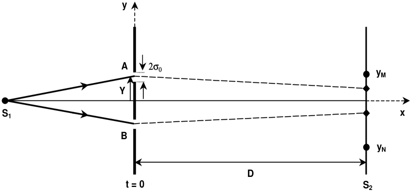
Figure 1: A two-slit experiment in which two identical entangled particles are emitted from the source $S_{1}$. Then, they pass through the slits $A$ and $B$, and finally they are detected on the screen $S_{2}$, simultaneously. We assumed that, $y_{0}=0$, or $\langle y_{0}\rangle=0$ under $\triangle y_{0}\ll\sigma_{0}$ and $\hbar t/2m\sigma_{0}^{2}\sim 1$ conditions. It is clear that dashed lines are not real trajectories.

We assumed that the two particles are entangled so that in spite of a position distribution for each particle, $y_{0}$ can be always considered to be on the $x$-axis. However, one may argue that, it is necessary to consider a position distribution for $y_{0}$, that is, $\triangle y_{0}\neq 0$ while $\langle y_{0}\rangle=0$. Therefore, it may seem that, not only symmetrical detection of the two particles is violated, but also they can be found at one side of the $x$-axis on the $S_{2}$ screen, because the majority of pairs can not be simultaneously on the $x$-axis [15]. Ghose [16] believes that the two entangled bosonic particles cannot cross the symmetry axis even if we have the situation $(y_{1}+y_{2})_{t=0}\neq 0$. However, by accepting Marchildon’s argument about this situation [15], this problem can be solved if we adjust $\triangle y_{0}$ to be very small and $\hbar t/2m\sigma_{0}^{2}\sim 1$. We assume that, to maintain symmetrical detection about the $x$-axis with reasonable approximation, the center of mass deviation from the $x$-axis must be smaller than the distance between any two neighbouring maxima on the screen $S_{2}$, that is,

$$\triangle y\ll\frac{\lambda D}{2Y}\simeq\frac{\pi\hbar t}{Ym},$$ (33)

where $\lambda$ is the de Broglie wavelength. For conditions $\hbar t/2m\sigma_{0}^{2}\sim 1$, $Y\sim\sigma_{0}$ and using equation (21), one obtains

$$\triangle y_{0}\ll\frac{\pi\hbar t}{Ym}\sim\sigma_{0}.$$ (34)

Therefore, if we use a source with $\triangle y_{0}\ll\sigma_{0}$, we will obtain $y\sim y_{0}\ll\sigma_{0}$ for each individual observation, and our symmetrical detection can be maintained with good approximation. In this case, we only lose our information about the trajectory of bosonic particles. It is evident that, if one considers $\triangle y_{0}\sim\sigma_{0}$, as was done in [15], the incompatibility between the two theories will disappear. But based on the entanglement of the two particles in the $y$-direction, we believe that, instead of the usual one-particle double-slit experiment with $\triangle y_{0}\sim\sigma_{0}$, our two-particle system provides a new situation in which we can adjust $y_{0}$ independent of $\sigma_{0}$, so that

$$0\leq y_{0}=\frac{1}{2}(y_{1}+y_{2})_{t=0}\ll\sigma_{0}.$$ (35)

Although it is obvious that $(\triangle y_{1})_{t=0}=(\triangle y_{2})_{t=0}\sim\sigma_{0}$, but the position entanglement of the two particles at the source $S_{1}$ in the $y$-direction makes them always satisfy equation (25), which is not feasible in the one-particle double-slit devices.

Now, one can compare the results of SQM and BQM at the ensemble level. To do this, we consider an ensemble of pairs of particles that have arrived at the detection screen $S_{2}$ at different times $t_{i}$. It is well known that, in order to ensure the compatibility between SQM and BQM for ensemble of particles, Bohm added a further postulate to his three basic and consistent postulates [1-3]. Based on this further postulate, the probability that a particle in the ensemble lies between $\overrightarrow{x}$ and $\overrightarrow{x}+d\overrightarrow{x}$, at time $t$, is given by

$$P(\overrightarrow{x},t)=R^{2}(\overrightarrow{x},t).$$ (36)

Thus, the joint probability of simultaneous detection for all pairs of particles of the ensemble arriving at $S_{2}$ is

$$P_{12}=\lim_{N\rightarrow\infty}\sum_{i=1}^{N}R^{2}(y_{1}(t_{i}),-y_{1}(t_{i}),t_{i})\equiv\int^{+\infty}_{-\infty}dy_{1}\int^{+\infty}_{-\infty}dy_{2}|\psi(y_{1},y_{2},t)|^{2}=1,$$ (37)

where every term in the sum shows only one pair arriving on the screen $S_{2}$ at the symmetrical points about the $x$-axis at time $t_{i}$, with the intensity of $R^{2}$. If all times $t_{i}$ in the sum are taken to be $t$, the summation on $i$ can be converted to an integral over all paths that cross the screen $S_{2}$ at that time, and we obtain an interference pattern. Then, one can consider the joint probability of detecting two particles at two arbitrary points $y_{M}$ and $y_{N}$ which can belong to different pairs

$$P_{12}(y_{M},y_{N},t)=\int_{y_{M}}^{y_{M}+\Delta}dy_{1}\int_{y_{N}}^{y_{N}+\Delta}dy_{2}|\psi(y_{1},y_{2},t)|^{2},$$ (38)

which is similar to the prediction of SQM, but obtained in a Bohmian way, as was shown by Ghose [12]. Thus, it appears that for such conditions, the possibility of distinguishing the two theories at the statistical level is impossible, as was expected [1-3, 9, 18].

Here, to show equivalence of the two theories, we have assumed for simplicity that $y_{0}=0$. If one consider $y_{0}\neq 0$ or $\triangle y_{0}\neq 0$, the equivalence of the two theories is maintained, as it is argued by Marchildon [15]. But, using this special case, we show that assumption of $y_{0}=0$ is consistent with statistical results of SQM and in consequence, finding such a source may not be impossible.

3.2 Predictions for the unentangled wave function

In this subsection, we complete our discussion by considering the unentangled wave function (10) and some of the Marchildon’s hints [15]. Based on equations (14) and (15), Bohmian velocities of particle 1 and 2 can be obtained as

$$\dot{y}_{1}= \widetilde{N} \frac{\hbar}{m}Im\{\frac{1}{(\psi_{A_{1}}+\psi_{B_{1}})}([\frac{-2(y_{1}-Y-u_{y}t)}{4\sigma_{0}\sigma_{t}}+ik_{y}]\psi_{A_{1}}$$ (39)

$$+ [\frac{-2(y_{1}+Y+u_{y}t)}{4\sigma_{0}\sigma_{t}}-ik_{y}]\psi_{B_{1}}\},$$ (40)

$$\dot{y}_{2}= \widetilde{N} \frac{\hbar}{m}Im\{\frac{1}{(\psi_{A_{2}}+\psi_{B_{2}})}([\frac{-2(y_{2}-Y-u_{y}t)}{4\sigma_{0}\sigma_{t}}+ik_{y}]\psi_{A_{2}}$$ (41)

$$+ [\frac{-2(y_{2}+Y+u_{y}t)}{4\sigma_{0}\sigma_{t}}-ik_{y}]\psi_{B_{2}}\},$$ (42)

Thus, as we expected, the speed of each particle is independent of the other. Using these relations as well as equations (18), we have

$$\dot{y}_{1}(x_{1},y_{1},t)=-\dot{y}_{1}(x_{1},-y_{1},t),$$ (43)

$$\dot{y}_{2}(x_{2},y_{2},t)=-\dot{y}_{2}(x_{2},-y_{2},t).$$ (44)

This implies that the $y$-component of the velocity of each particle would vanish on the $x$-axis. Although these relations are similar to the relations that were obtained for the entangled wave function, but here we have an advantage: none of the particles can cross the $x$-axis nor are tangent to it, independent of the other particle’s position. This property can be used to show that BQM’s predictions are incompatible with SQM’s.

To see this incompatibility, we use a special detection process on the screen $S_{2}$ that we call it selective detection. In the selective detection, we register only those pair of particles which are detected on the two sides of the $x$-axis, simultaneously. That is, we eliminate the cases of detecting only one particle or detecting both particles of the pair on the upper or lower part of the $x$-axis on the screen. Again, it is useful to obtain the equation of motion of the center of mass in the $y$-direction. Using equation (29) and (30), one can show that,

$$\dot{y}=\frac{(\hbar/2m\sigma_{0}^{2})^{2}t(y_{1}+y_{2})/2}{1+(\hbar/2m\sigma_{0}^{2})^{2}t^{2}}+\widetilde{N}\frac{\hbar}{2m}Im\{\frac{1}{\psi}(\frac{Y+u_{y}t}{\sigma_{0}\sigma_{t}}+2ik_{y})(\psi_{A_{1}}\psi_{A_{2}}-\psi_{B_{1}}\psi_{B_{2}})\}.$$ (45)

We can assume that the distance between the source and the two-slit screen is so large that we have $k_{y}\simeq 0$. Then, using the special case $Y\ll\sigma_{0}$, the second term in eq. (32) becomes negligible and the equation of motion for the $y$-coordinate of the center of mass is reduced to

$$\dot{y}\simeq\frac{(\hbar/2m\sigma_{0}^{2})^{2}}{1+(\hbar/2m\sigma_{0}^{2})^{2}t^{2}}yt,$$ (46)

and similar to the last experiment, we have

$$y\simeq y_{0}\sqrt{1+(\hbar/2m\sigma_{0}^{2})^{2}t^{2}}.$$ (47)

Since for this special source there was not any entanglement between the two particles, we must have $\triangle y_{0}\sim\sigma_{0}$. Consider the case in which $\langle y_{0}\rangle=0$. To obtain symmetrical detection with reasonable approximation, we consider $\hbar t/2m\sigma_{0}^{2}\sim 1$ so that $y\sim y_{0}$. Then, according to eq. (23), one can write

$$\triangle y_{0}\ll\frac{\pi\hbar t}{Ym},$$ (48)

which yields

$$Y\ll 2\pi\sigma_{0}.$$ (49)

Therefore, under these conditions, BQM’s symmetrical prediction is incompatible with SQM’s asymmetrical prediction. Figure 2 shows a schematic drawing of BQM’s symmetrical detection occurred at the first maximum for the condition $Y\ll 2\pi\sigma_{0}$.

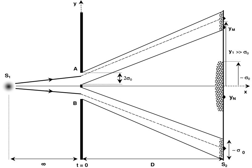
Figure 2: Schematic drawing of a two-slit experiment in which two identical unentangled particles are emitted by the source $S_{1}$. The symmetrical detection is not predicted at the central maxima, using both SQM and BQM. But, we have symmetrical detection at the other maxima (for example, at $y_{1}$ as the first maxima) under the condition $Y\ll 2\pi\sigma_{0}$, using BQM.

Now, consider conditions under which $y_{0}\neq 0$ and $\hbar t/2m\sigma_{0}^{2}\gg 1$. Then, the $x$-axis will not be an axis of symmetry and we have a new point on the $S_{2}$ screen along the $y$-axis around which all pairs of particles will be detected symmetrically. Thus, based on BQM, that is relations (31) and (34), there will be an empty interval

$$L=2y\simeq\frac{\hbar ty_{0}}{m\sigma_{0}^{2}},$$ (50)

on the screen $S_{2}$ where no particle is recorded. But, one can argue that the quantum distribution of the two particles does not allow to form the empty interval on the screen. Thus, assume that $\langle y_{0}\rangle\neq 0$ and $\triangle y_{0}\sim\sigma_{0}$. Then, we can have a relative empty interval of low intensity particles that has a length

$$L\simeq 2\langle y\rangle\simeq\frac{\hbar t}{m\sigma_{0}^{2}}\langle y_{0}\rangle,$$ (51)

if $\triangle y\ll L$ condition is satisfied. It is obvious that, the last condition corresponds to $\triangle y_{0}\ll\langle y_{0}\rangle$. Therefore, it is seen that, using BQM and under the condition

$$Y\ll\sigma_{0}\ll\langle y_{0}\rangle,$$ (52)

a considerable change in the position of the source $S_{1}$ toward positive (negative) $y$-direction produces a region with very low intensity in the interference pattern above (below) the $x$-axis which cannot be predicted by SQM, as is shown in Figure 3.

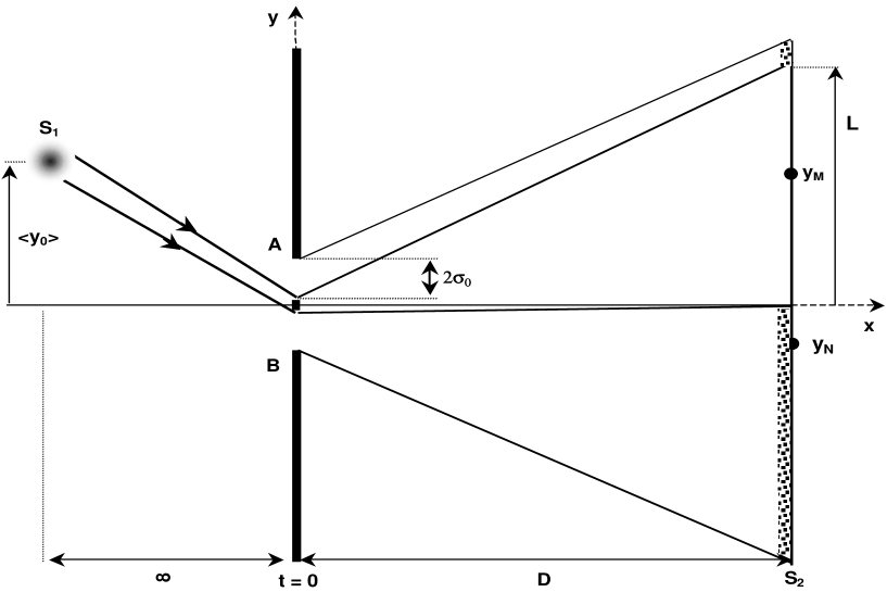
Figure 3: Schematic drawing of a two-unentangled particle two-slit experiment in which the conditions $Y\ll\sigma_{0}\ll\langle y_{0}\rangle$ and $\hbar t/2m\sigma_{0}^{2}\gg 1$ along with selective detection are considered. The length $L$ shows the empty interval in the final interference pattern.

However, based on SQM, we have two alternatives:
i) The joint probability relation (11) is still valid and there is only a reduction in the intensity throughout the screen $S_{2}$, due to the selective detection.
ii) SQM is silent about our selective detection.
In the first case, there is a disagreement between the predictions of SQM and BQM and in the second case, BQM has a better predictive power than SQM, even at the statistical level.

It is worthy to note that, based on our factorizable wave function (10), one may object that each particle simply follows one of the single-particle two-slit trajectories and is quite independent of the other particle and in consequence, both SQM and BQM must yield the same results. But, one can see that this objection is unfounded for our specified conditions in which we have used the guidance condition along with the selective detection. If we study the interference pattern without using selective detection, we must obtain the same results for the two theories. But, using selective detection, it is clear that not only the two theories do not have the same statistical predictions, but also BQM clarifies and illuminates SQM, as Durr et al. [18] said:“note that by selectively forgetting results we can dramatically alter the statistics of those that we have not forgotten. This is a striking illustration of the way in which Bohmian mechanics does not merely agree with the quantum formalism, but, eliminating ambiguities, clarifies, and sharpens it.”. In our selective detection, we have forgotten detected single-particle and two-particle contributions at the one side of the $x$-axis on the screen $S_{2}$. Elsewhere [17], we have also shown that there is another statistical disagreement between the two theories for a new two-particle system described by an entangled wave function, using a different selective detection and without any deviation of the source from the $x$-axis. Therefore, it seems that performing such experiments provides observable differences between the two theories, particularly at the statistical level.

4 Conclusion

In this article, we have suggested two thought experiments to distinguish between the standard and the Bohmian quantum mechanics. The suggested experiments consist of a two-slit interferometer with a special source which emits two identical non-relativistic particles. We have shown that, according to the characteristic of the source, our two-particle system can be described by two kinds of wave functions: the entangled and the unentangled wave functions. For the entangled wave function, we have obtained some disagreement between SQM and BQM at the individual level. But, it is shown that, the two theories predict the same statistical results, as expected. For the unentangled wave function, the predictions of the two theories could be different at the individual level too. Again, the results of the two theories were the same at the ensemble level. However, the use of selective detection can dramatically alter the interference pattern, so that not only the statistical results of BQM do not agree with those of SQM, but BQM can also increase our predictive power. Therefore, it seems that, our suggested thought experiments can decide between the standard and the Bohmian quantum mechanics.

References

- [1] D. Bohm, Part I, Phys. Rev. 85 (1952) 166; Part II, 85 (1952) 180.
- [2] D. Bohm and B.J. Hiley, The Undivided Universe, Routledge, London, 1993.
- [3] P.R. Holland, The Quantum Theory of Motion, Cambridge University Press, Cambridge, 1993.
- [4] J.T. Cushing, Quantum Mechanics: Historical Contingency and the Copenhagen Hegemony, The University of Chicago Press, Ltd., London, 1994.
- [5] M. Abolhasani and M. Golshani, Phys. Rev. A 62 (2000) 12106.
- [6] B.G. Englert, M.O. Scully, G. Sussman and H. Walther, Z. Naturforsch. 47a (1992) 1175.
- [7] M.O. Scully, Phys. Scripta, T 76 (1998) 41.
- [8] C. Dewdney, L. Hardy and E.J. Squires, Phys. Lett. A 184 (1993) 6.
- [9] B.J. Hiley, R.E. Callaghan and O.J.E. Maroney, Quantum Trajectories, Real, Surreal or an Approximation to a Deeper Process?, quant-ph/0010020.
- [10] J.P. Vigier, Phys. Lett. A 270 (2000) 221.
- [11] A.J. Leggett, Found. Phys. 29 (1999) 445.
- [12] P. Ghose, Incompatibility of the de Broglie-Bohm Theory with Quantum Mechanics, quant-ph/0001024; An Experiment to Distinguish Between de Broglie-Bohm and Standard Quantum Mechanics, quant-ph/0003037.
- [13] M. Golshani and O. Akhavan, A two-slit experiment which distinguishes between standard and Bohmian quantum mechanics, quant-ph/0009040.
- [14] L. Marchildon, No contradictions between Bohmian and quantum mechanics, quant-ph/0007068.
- [15] L. Marchildon, On Bohmian trajectories in two-particle interfrence devices, quant-ph/0101132.
- [16] P. Ghose, Comments on“On Bohm trajectories in two-particle interference devices” by L. Marchildon, quant-ph/0102131.
- [17] M. Golshani and O. Akhavan, J. Phys. A 34 (2001) 5259, quant-ph/0103101.
- [18] D. Durr, S. Goldstein and N. Zanghi, J. Stat. Phys. 67 (1992) 843.