Peculiarities of the Weyl - Wigner - Moyal formalism for scalar charged particles

Abstract

A description of scalar charged particles, based on the Feshbach - Villars formalism, is proposed. Particles are described by an object that is a Wigner function in usual coordinates and momenta and a density matrix in the charge variable. It is possible to introduce the usual Wigner function for a large class of dynamical variables. Such an approach explicitly contains a measuring device frame. From our point of view it corresponds to the Copenhagen interpretation of quantum mechanics. It is shown how physical properties of such particles depend on the definition of the coordinate operator. The evolution equation for the Wigner function of a single-charge state in the classical limit coincides with the Liouville equation. Localization peculiarities manifest themselves in specific constraints on possible initial conditions.

I Introduction

The question regarding the nature of the wavefunction has its origin in the early years of quantum mechanics. For a long time it has been considered as a philosophical rather then a physical question [1, 2, 3]. However, it is now very real because of the recent theoretical and experimental progress in quantum information [2, 4, 5].

One of the significant points in understanding the nature of the wave function is the Einstein - Podolsky - Rosen paradox and the existence of quantum correlations related to it. Since 1980, such specific behavior of quantum systems has been confirmed many times in experiments [6]. It is very important that such correlations ”spread” in space instantly. Nevertheless, if one adheres to the Copenhagen interpretation, there is no violation of causality principle.

However, due to the fact that collapse of the wavefunction takes place at a given instant (or maybe in a small time interval) in the whole space, one can speak of violation of causality principle and a conflict between quantum mechanics and special relativity [7, 8] in some interpretations of quantum mechanics. Following the idea of Bell and Eberhard that a consistent description should contain a preferred frame, relativistic classical and quantum mechanics is built in [9, 10] in such a way that the relativity principle is generalized and the causality is not violated. A basic assumption of this theory is that transformation from one frame to another is realized by operators which are isomorphic to the Lorentz group and depend on a certain four-vector (as parameter) in such a way that the instant time hyper-plain is invariant. This vector is interpreted as a relative to an observer four-velocity of the preferred frame. Under this assumption the postulate about the light speed constancy is changed to the postulate about the constancy of the average speed of light on closed path.

One of the remarkable peculiarities of this theory is in the existence of a well-defined position operator [10] which coincides with the Newton - Wigner position operator [11, 12] in the preferred frame. It means that in this approach measurement of position does not create a particle - antiparticle couple since the odd part responsible for appearance of a different charge state superposition is absent. Hence, there exists a supposition that localization of relativistic particles can bear information about presence of the preferred frame in the Universe.

The above arguments show the fundamental role that determination of the position operator structure can play. Moreover, the question of whether it is a one-particle, or, in principle, a many-particle operator, is of specific interest as well. Therefore, it is very important to find situations where the odd part of the position operator could manifest itself. It would be possible to realize such observation on strongly localized (near the Compton wavelength) states of a separate particle. However, because such states are a problem for laboratory experiments, it is of great interest how this peculiarity manifests itself in a many-particle system.

The Weyl - Wigner - Moyal (WWM) formalism is a convenient method to describe both one-particle and many-particle quantum systems in non-relativistic theory [13, 14, 15, 16]. Nevertheless, attempts to generalize it for the relativistic case lead to a number of problems. The first problem is that the Weyl rule [17] does not include time as a dynamical variable, and the scalar product in the Hilbert space of states is formulated for functions square integrable not over the whole space-time but in the three-dimensional space or in a space-like hyper-surface only. In [18] this problem was resolved by generalization of the spatial integration over the whole space-time without Weyl rule application. The WWM formalism in the framework of the stochastic formulation of quantum mechanics, where the scalar product is formulated for square integrable functions in the whole space-time, also leads to Lorenz-invariant expressions [19].

The matrix-valued Wigner function formalism has been developed for the general case of many component equations and, in particular, for $1/2$ spin particles on the basis of the usual Weyl rule [20, 21]. Certainly, such equations are not Lorenz invariant, though average values coincide with their analogues in the usual approach.

The next essential problem in relativistic WWM formalism is in absence of a well-defined position operator. Unlike the works mentioned above, where the Wigner function is determined by means of the usual position operator, in [22, 23] a formalism with the Newton - Wigner position operator is developed. This approach is not Lorenz invariant either, and respective results differ from the standard ones. However, they can be related to [10], where the consistent definition of the position operator is possible.

The goals of this paper are in formulating the WWM relativistic formalism for scalar charged particles under the approach of [20] and finding a set of specific peculiarities in relativistic quantum system behavior, that are related to the non-trivial structure of the position operator. It turns out that values of some observables depend directly on the position operator definition, that, as mentioned above, can be a consequence of existence of the preferred frame in the Universe.

In Sec.II we introduce the Weyl rule for matrix-valued observables in the case of scalar charged particles and discuss peculiarities of correspondence between classical and quantum dynamical algebras. Sec.III is devoted to the matrix-valued Wigner function and quantum Liouville equation. Here we also discuss the absence of Lorenz invariance of this approach, and how it can be related to the Copenhagen interpretation of quantum mechanics. In Sec.IV we consider how the usual Weyl rule turns into the Feshbach - Villars representation. Among the whole set of dynamical variables, we separate a special class of observables with the Weyl symbols independent of charge variable (charge-invariant variables). They have several remarkable properties. In particular, we find the relationship between their even and odd parts. The usual (not matrix-valued) Wigner function can be introduced for such observables. It is considered in Sec.V (for a brief abstract of this approach see [24]). This object includes four components: one corresponds to a particle, second one corresponds to an antiparticle (even part of Wigner function), and two more are interference terms (odd part of Wigner function). The evolution equation for the odd part becomes zero in the classical limit, and the equation for the even part coincides with its analogue in the Newton - Wigner position operator approach [22, 23]. The difference reveals itself in peculiarities of constraints on initial conditions that are considered in Sec.VI.

II Weyl rule and specific properties of dynamical algebra for scalar charged particles

In this and the following Sections we apply the methods developed in [20, 21] to the Klein - Gordon equation that is written using the Feshbach - Villars formalism [12]. This makes it possible to take the charge variable into account explicitly. With account of the fact that the Hilbert space of states for scalar charged particles has an indefinite metric, we have to distinguish between covariant and contravariant basis vectors and coordinates for subspace corresponding to the charge variable. Hence, arbitrary state is expanded on basis vectors in the following way:

$$\left|\Psi\right\rangle=\sum\limits_{\alpha=\pm 1}{\left|{\Psi^{\alpha}}\right\rangle\otimes\left|{e_{\alpha}}\right\rangle},$$ (1)

where

$$\left|{\Psi^{\alpha}}\right\rangle=\sum\limits_{s}{\Psi^{\alpha}(s)\left|s\right\rangle}.$$ (2)

Here $s=q,p,...$ is an arbitrary dynamical variable and the summarizing symbol can be interpreted as an integration with respect to $s$. Greek indices take values $\pm 1$. $\tau_{3}{}_{\alpha\beta}$ plays the role of metric tensor (see [12]). In notations like $\delta_{\alpha}{}^{\beta}$, $\tau_{1_{\alpha}\beta}$, $\tau_{2\alpha\beta}$, $\tau_{3\alpha\beta}$, $\tau_{3}{}_{\alpha}{}^{\beta}$,…, symbols $\delta$, $\tau_{i}$ do not correspond to specific operators and mean only values of the corresponding matrix elements. There are some peculiarities in notations of operators as well. $\hat{A}$ is a full operator that acts on all dynamical variables. $\check{A}$ is an operator that acts on the charge variables only (or, in other words, it is a $c$-numeric matrix).

For a consistent development of the WWM formalism we shall formulate the Weyl rule bringing into correspondence matrix-valued classical variables (Weyl symbols) to quantum-mechanical operators. Here we should take into account that in our case classical variables are operators acting on the charge variable. However, because the operator of quasi-probability density in the coordinate representation is proportional to the identity matrix in charge space, the succession of this operator and a matrix-valued Weyl symbol does not matter. Choosing it in an arbitrary way, one can write the Weyl rule as follows:

$$\hat{A}_{\alpha}{}^{\beta}=\sum\limits_{\gamma=\pm 1}{\int\limits_{-\infty}^{+\infty}{A_{\gamma}{}^{\beta}(p,q)\hat{W}_{\alpha}{}^{\gamma}(p,q)dpdq}},$$ (3)

where $A_{\alpha}{}^{\beta}(p,q)$ is the matrix-valued Weyl symbol, $\hat{A}_{\alpha}{}^{\beta}$ stands for corresponding quantum-mechanical operator, $\hat{W}_{\alpha}{}^{\beta}(p,q)$ is the operator of quasi-probability density that is the Fourier transform of the displacement operator. Following [16] one can obtain the expansion of $\hat{W}_{\alpha}{}^{\beta}(p,q)$ on eigenvectors of the position operator:

$$\hat{W}_{\alpha}{}^{\beta}(p,q)=\frac{1}{{(2\pi\hbar)^{d}}}\int\limits_{-\infty}^{+\infty}{\left|{q+\frac{Q}{2}}\right\rangle\delta_{\alpha}{}^{\beta}\exp\left[\frac{i}{\hbar}Qp\right]dQ\left\langle{q-\frac{Q}{2}}\right|},$$ (4)

where $d=3$ is dimensionality of the physical space.

Substituting (4) to (3) one can find the expression for an arbitrary operator expansion:

$$\hat{A}_{\alpha}{}^{\beta}=\frac{1}{{(2\pi\hbar)^{d}}}\int\limits_{-\infty}^{+\infty}{\left|{q+\frac{Q}{2}}\right\rangle A_{\alpha}{}^{\beta}(p,q)}\exp\left[\frac{i}{\hbar}Qp\right]dQdpdq\left\langle{q-\frac{Q}{2}}\right|.$$ (5)

Similarly, such expression can be written by expending the operator of quasi-probability density on the eigenvectors of the momentum operator:

$$\hat{A}_{\alpha}{}^{\beta}=\frac{1}{{(2\pi\hbar)^{d}}}\int\limits_{-\infty}^{+\infty}{\left|{p+\frac{P}{2}}\right\rangle A_{\alpha}{}^{\beta}(p,q)\exp\left[-\frac{i}{\hbar}Pq\right]dPdpdq\left\langle{p-\frac{P}{2}}\right|}.$$ (6)

Matrix elements of this operator can be found in the form:

$$\left\langle{q_{1}}\right|\hat{A}_{\alpha}{}^{\beta}\left|{q_{2}}\right\rangle=\frac{1}{{(2\pi\hbar)^{d}}}\int\limits_{-\infty}^{+\infty}{A_{\alpha}{}^{\beta}(p,\frac{1}{2}(q_{1}+q_{2}))\exp\left[\frac{i}{\hbar}(q_{1}-q_{2})p\right]dp}.$$ (7)

By changing variables in this expression in a standard way and performing Fourier transformation one can obtain the expression that reconstructs matrix-valued Weyl symbol through operator:

$$A_{\alpha}{}^{\beta}(p,q)=\int\limits_{-\infty}^{+\infty}{\left\langle{q+\frac{Q}{2}}\right|\hat{A}_{\alpha}{}^{\beta}\left|{q-\frac{Q}{2}}\right\rangle\exp\left[-\frac{i}{\hbar}Qp\right]dQ}.$$ (8)

In [22] the integral form of the Klein - Gordon equation with pseudo-differential symbols in the Feshbach - Villars representation (where Hamiltonian matrix has a diagonal form) is obtained. In fact, it means that the Newton - Wigner coordinate is used there instead of the usual coordinate. Here we obtain another integral form of the Klein - Gordon equation using the usual position operator:

$$i\hbar\partial_{t}\Psi_{\alpha}(x)=\frac{1}{{(2\pi\hbar)^{d}}}\sum\limits_{\beta=\pm 1}{\int\limits_{-\infty}^{+\infty}{H^{\beta}{}_{\alpha}(p,\frac{1}{2}(x+y))\exp\left[\frac{i}{\hbar}(x-y)p\right]\Psi_{\beta}(y)dpdy}},$$ (9)

where

$$H^{\beta}{}_{\alpha}(p,x)=(\tau_{3}{}^{\beta}{}_{\alpha}+i\tau_{2}{}^{\beta}{}_{\alpha})\frac{{(\vec{p}-e\vec{A}(x))^{2}}}{{2m}}+\tau_{3}{}^{\beta}{}_{\alpha}mc^{2}+e\varphi(x)\delta^{\beta}{}_{\alpha}$$ (10)

is the matrix-valued Weyl symbol of the Hamiltonian in the general case (for a particle in electromagnetic field), which depends on both coordinate and momentum. Unlike [22] this equation takes into account that the position operator mixes states with different charge signs.

Until now,consideration of the matrix-valued WWM formalism has been very similar to the usual one. Considerable differences appear in determining the matrix-valued Moyal bracket and in the classical limit. To consider this question one should find the matrix-valued Weyl symbol from the product of two operators in a standard way.

Let $\check{A}(p,q)$ and $\check{B}(p,q)$ be matrix-valued Weyl symbols of two operators $\hat{A}$ and $\hat{B}$ respectively. Let us introduce operators $\hat{C}_{1},\hat{C}_{2},\hat{C}$ as follows:

$$\begin{array}[]{l}\hat{C}_{1}=\hat{A}\hat{B}\\ \hat{C}_{2}=\hat{B}\hat{A}\\ \hat{C}=[\hat{A},\hat{B}]=\hat{C}_{1}-\hat{C}_{2}\end{array}.$$ (11)

Then, using (8) and consideration like that used in [15], one can obtain the matrix-valued Weyl symbol of the operator $\hat{C}_{1}$:

$$\check{C}_{1}(p,q)=\check{A}(p,q)\exp\left[\frac{{i\hbar}}{2}(\overleftarrow{\partial}_{q}\overrightarrow{\partial}_{p}-\overleftarrow{\partial}_{p}\overrightarrow{\partial}_{q})\right]\check{B}(p,q).$$ (12)

For the matrix-valued Weyl symbol of the operator $\hat{C}_{2}$ one can find a similar expression. Therefore, the matrix-valued Moyal bracket can be determined in the following form:

$$\begin{array}[]{l}\{\check{A}(p,q),\check{B}(p,q)\}_{M}=\frac{1}{{i\hbar}}\check{C}(p,q)=\\ =\frac{1}{{i\hbar}}\left({\check{A}(p,q)\exp\left[\frac{{i\hbar}}{2}(\overleftarrow{\partial}_{q}\overrightarrow{\partial}_{p}-\overleftarrow{\partial}_{p}\overrightarrow{\partial}_{q})\right]\check{B}(p,q)-\check{B}(p,q)\exp\left[\frac{{i\hbar}}{2}(\overleftarrow{\partial}_{q}\overrightarrow{\partial}_{p}-\overleftarrow{\partial}_{p}\overrightarrow{\partial}_{q})\right]\check{A}(p,q)}\right)\end{array}.$$ (13)

Unlike the usual case, matrix-valued Weyl symbols do not commutate, so it is not possible to represent such a Moyal bracket as a sinus from the operator of the Poisson bracket. This fact results in the classical limit in some peculiarities. In the general case, one can express the classical limit of the matrix-valued Moyal bracket via the matrix-valued Poisson bracket [21] and the commutator of the matrix-valued Weyl symbols:

$$\mathrel{\mathop{\lim}\limits_{\hbar\rightarrow 0}}{{\{\check{A},\check{B}\}}_{M}}=\frac{1}{{i\hbar}}[\check{A},\check{B}]+\frac{1}{2}\left({\{\check{A},\check{B}\}_{P}-\{\check{B},\check{A}\}_{P}}\right).$$ (14)

If the matrix-valued Weyl symbols (for example position and Hamiltonian) commutate, the matrix-valued Moyal bracket is in fact the usual one and coincides with the Poisson bracket in the classical limit. If they do not commutate with each other, three cases are possible. Let $[\check{A},\check{B}]=O\left({\hbar^{\nu}}\right)$ when $\hbar\to 0$. If $\nu<1$, the classical limit does not exist for such a couple of the matrix-valued Weyl symbols, since the value of the matrix-valued Moyal bracket increases infinitely. If $\nu>1$, it becomes zero in the classical limit. If $\nu=1$, the classical limit exists. Here we can take as an example the Newton -Wigner position operator [11, 12]. Part of its matrix-valued Weyl symbol,not commutating with the Hamiltonian, is proportional to Planck’s constant, thus in this case there exists a well-defined classical limit.

III Matrix-valued Wigner function and quantum Liouville equation

Using (3), one can find the average value of an arbitrary operator $\hat{A}$ expressed via its matrix-valued Weyl symbol:

$$\bar{A}=\sum\limits_{\alpha,\beta,\gamma=\pm 1}{\int\limits_{-\infty}^{+\infty}{A_{\gamma}{}^{\beta}(p,q)\left\langle{\Psi_{\beta}}\right|\hat{W}_{\alpha}{}^{\gamma}(p,q)\left|{\Psi^{\alpha}}\right\rangle dpdq}}.$$ (15)

Then, introducing the matrix-valued Wigner function

$$W_{\beta}{}^{\gamma}(p,q)=\sum\limits_{\alpha=\pm 1}{\left\langle{\Psi_{\beta}}\right|\hat{W}_{\alpha}{}^{\gamma}(p,q)\left|{\Psi^{\alpha}}\right\rangle},$$ (16)

this expression can be written in a simpler form:

$$\bar{A}=tr\int\limits_{-\infty}^{+\infty}{\check{A}(p,q)\check{W}(p,q)dpdq}.$$ (17)

Substitution of the operator of quasi-probability density expansion (4) into (16) leads to the expression for the matrix-valued Wigner function in the coordinate representation. As a result we obtain a formula that coincides with the definition given in [20]:

$$W_{\alpha}{}^{\beta}(p,q)=\frac{1}{{(2\pi\hbar)^{d}}}\int\limits_{-\infty}^{+\infty}{\Psi_{\alpha}^{\ast}(q+\frac{Q}{2})\Psi^{\beta}(q-\frac{Q}{2})\exp\left[\frac{i}{\hbar}Qp\right]dQ}.$$ (18)

Next, let us describe a method to obtain evolution equation for the matrix-valued Wigner function of a scalar charged particle. To do this one shall differentiate expression (18) with respect to time. The value of the wavefunction derivative is taken from the integral form of the Klein - Gordon equation (9). After standard transformations, similar to the usual WWM formalism, we obtain the quantum Liouville equation

$$\partial_{t}{\check{W}}=\{\check{H},\check{W}\}_{M},$$ (19)

where the matrix-valued Moyal bracket is determined by expression (13).

At first sight, this equation has a considerable defect in comparison to similar expressions in [18, 19]; namely, it is not Lorentz invariant. For an interpretation of this fact, we have to take into account arguments from the measurement theory. The fact is that average values calculated in this approach coincide with ones in the usual (Schrödinger) representation of quantum mechanics that is Lorentz invariant. Nevertheless, unlike the stochastic formulation of quantum mechanics [25], the scalar product is determined here with functions that are square integrable in a certain space-like hyper-surface, rather than over the whole space-time. Moreover, the value of scalar product does not depend on its choice [26]. One can relate this hyper-surface to the measurement device frame. In other words, the wavefunction collapse occurs in a frame in which equation (19) is written. The absence of Lorentz invariance is a consequence of the fact that the Weyl rule does not include time as an independent dynamical variable.

In [27] the process of relativistic measurement is considered. In that work the point of view is expressed, that the wavefunction (and as result the Wigner function, we notice) has no objective value and does not covariantly transform when there are classical interventions. Here we note that in principle equation (19) can be written with four-dimensional Lorentz invariant symbols only, but to do this we have to incorporate in the theory a certain time-like unit vector in a way similar to Tomonaga-Schwinger approach to quantum field theory [28, 29]. It is the four-velocity of the frame where the wavefunction collapse occurs (the measuring device frame) relative to the second static observer (watching observer). This frame has principally another sense to that of the preferred frame in [7, 8, 9, 10]. In that approach [9, 10] collapse of the wavefunction has to take place in all frames in the whole space (because of the instant time hyper-surface being invariant). In our approach this process obeys the relativity of simultaneity. If it were possible to observe the wave function directly, such a hypothetical watching observer would see the wavefunction collapse as a certain moving front. As a result, at a certain instant, in a static frame (attached to the watching observer), a state with a part of the wavefunction before measurement on one hand and a part of the wavefunction after measurement on the other hand, is realized (Fig.1). But perhaps it is impossible to propose even gedanken experiment without use of a superluminar signal to interpret the results in favor of one of the approaches.

Hence we find to be very important and of fundamental value the fact that quantum mechanics in the Wigner representation necessarily includes the four-velocity of the measuring device frame in explicit form.

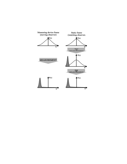
FIG. 1.: The process of the wavefunction collapse in a moving frame from points of view of an observer in this frame and a static observer (watching observer). For the latter this process is a certain moving front. At a certain instant a state exists where at one side (right) there is the wavefunction before the measurement and on the other side (left) there is the wavefunction after the measurement.

IV Transformation to the Feshbach - Villars representation

In the Feshbach - Villars representation, Hamiltonian matrix has a diagonal form and indices in the charge space correspond to the particle and antiparticle [12]. Therefore, it is convenient to distinguish between solutions with different charge signs and to give them explicit physical sense. Furthermore, in this approach an influence of the odd part of the position operator on values of some physical variables is more evident.

Operator $\hat{A}_{\alpha}{}^{\beta}$transforms to the Feshbach - Villars representation by the following formula:

$$\hat{A}^{FV}{}_{\alpha}{}^{\beta}=\sum\limits_{\gamma,\delta=\pm 1}{\hat{U}_{\gamma}{}^{\beta}\hat{A}_{\delta}{}^{\gamma}\hat{U}^{-1}{}_{\alpha}{}^{\delta}},$$ (20)

where the transformation matrix has the form:

$$\hat{U}_{\alpha}{}^{\beta}(\hat{p})=\frac{1}{{2\sqrt{mc^{2}E(\hat{p})}}}\left[{(E(\hat{p})+mc^{2})\delta_{\alpha}{}^{\beta}+(E(\hat{p})-mc^{2})\tau_{1}{}_{\alpha}{}^{\beta}}\right].$$ (21)

Here and below

$$E(p)=\left(m^{2}c^{4}+c^{2}p^{2}\right)^{\frac{1}{2}}$$ (22)

is the energy of a relativistic free particle.

Next, we apply (20) to the Weyl rule in the form (6). As result, we obtain the expression that brings into correspondence the matrix-valued Weyl symbol to the operator in the Feshbach-Villars representation:

$$\hat{A}^{FV}{}_{\alpha}{}^{\beta}=\frac{1}{{(2\pi\hbar)^{d}}}\int\limits_{-\infty}^{+\infty}{\left|{p+\frac{P}{2}}\right\rangle}\sum\limits_{\gamma,\delta=\pm 1}{U_{\gamma}{}^{\beta}(p+\frac{P}{2})A_{\delta}{}^{\gamma}(p,q)U^{-1}{}_{\alpha}{}^{\delta}(p-\frac{P}{2})\exp\left[-\frac{i}{\hbar}Pq\right]dPdpdq\left\langle{p-\frac{P}{2}}\right|}.$$ (23)

In general, it is rather difficult to interpret this expression since there is a complicated dependence on the integration variable under the integral sign. Here we do not go beyond the simplest case.

Let the matrix-valued Weyl symbol be proportional to the identity matrix:

$$A_{\alpha}{}^{\beta}(p,q)=A(p,q)\delta_{\alpha}{}^{\beta}.$$ (24)

In principle, one can say that such symbols do not depend on the charge variable, so that the class of dynamical variables, which corresponds to those, we denominate here, to be more brief, as a class of charge-invariant variables. Most of the dynamical variables that we consider in relativistic (non-quantum) mechanics belong to this class. The reason for this is the absence of a dependence on the charge variable in classical mechanics. Hence, the question about the classical limit is for such variables especially interesting.

The Weyl rule for charge-invariant variables in the Feshbach - Villars representation has the form:

$$\hat{A}^{FV}{}_{\alpha}{}^{\beta}=\frac{1}{{(2\pi\hbar)^{d}}}\int\limits_{-\infty}^{+\infty}{\left|{p+\frac{P}{2}}\right\rangle A(p,q)R_{\alpha}{}^{\beta}(p+\frac{P}{2},p-\frac{P}{2})\exp\left[-\frac{i}{\hbar}Pq\right]dPdpdq\left\langle{p-\frac{P}{2}}\right|}.$$ (25)

Unlike [23] and non-relativistic case there is a matrix-valued variable here:

$$R_{\alpha}{}^{\beta}(p_{1},p_{2})=\varepsilon(p_{1},p_{2})\delta_{\alpha}{}^{\beta}+\chi(p_{1},p_{2})\tau_{1}{}_{\alpha}{}^{\beta}.$$ (26)

It contains even and odd parts and is expressed via the energy of a free particle (22):

$$\begin{tabular}[]{l}$\varepsilon(p_{1},p_{2})=\frac{{E(p_{1})+E(p_{2})}}{{2\sqrt{E(p_{1})E(p_{2})}}}$\\ $\chi(p_{1},p_{2})=\frac{{E(p_{1})-E(p_{2})}}{{2\sqrt{E(p_{1})E(p_{2})}}}$\end{tabular}.$$ (27)

Consequences from (25) are expressions for even $[\hat{A}]$ and odd $\{\hat{A}\}$ parts of the operator of a charge-invariant observable in terms of its Weyl symbol:

$$\left[\hat{A}^{FV}\right]_{\alpha}{}^{\beta}=\frac{1}{{(2\pi\hbar)^{d}}}\int\limits_{-\infty}^{+\infty}{\left|{p+\frac{P}{2}}\right\rangle A(p,q)\varepsilon(p+\frac{P}{2},p-\frac{P}{2})\delta_{\alpha}{}^{\beta}\exp\left[-\frac{i}{\hbar}Pq\right]dPdpdq\left\langle{p-\frac{P}{2}}\right|},$$ (28)

$$\left\{\hat{A}^{FV}\right\}_{\alpha}{}^{\beta}=\frac{1}{{(2\pi\hbar)^{d}}}\int\limits_{-\infty}^{+\infty}{\left|{p+\frac{P}{2}}\right\rangle A(p,q)\chi(p+\frac{P}{2},p-\frac{P}{2})\tau_{1}{}_{\alpha}{}^{\beta}\exp\left[-\frac{i}{\hbar}Pq\right]dPdpdq\left\langle{p-\frac{P}{2}}\right|.}$$ (29)

Matrix elements with eigenvectors of the momentum of the operator of a charge-invariant variable and its even and odd parts can be written in the following form:

$$\left\langle{p_{1}}\right|\hat{A}^{FV}{}_{\alpha}{}^{\beta}\left|{p_{2}}\right\rangle=\frac{1}{{(2\pi\hbar)^{d}}}R_{\alpha}{}^{\beta}(p_{1},p_{2})\int\limits_{-\infty}^{+\infty}{A(\frac{1}{2}(p_{1}+p_{2}),q)\exp\left[-\frac{i}{\hbar}(p_{1}-p_{2})q\right]dq},$$ (30)

$$\left\langle{p_{1}}\right|\left[\hat{A}^{FV}\right]_{\alpha}{}^{\beta}\left|{p_{2}}\right\rangle=\frac{1}{{(2\pi\hbar)^{d}}}\varepsilon(p_{1},p_{2})\delta_{\alpha}{}^{\beta}\int\limits_{-\infty}^{+\infty}{A(\frac{1}{2}(p_{1}+p_{2}),q)\exp\left[-\frac{i}{\hbar}(p_{1}-p_{2})q\right]dq},$$ (31)

$$\left\langle{p_{1}}\right|\left\{\hat{A}^{FV}\right\}{}_{\alpha}{}^{\beta}\left|{p_{2}}\right\rangle=\frac{1}{{(2\pi\hbar)^{d}}}\chi(p_{1},p_{2})\tau_{1}{}_{\alpha}{}^{\beta}\int\limits_{-\infty}^{+\infty}{A(\frac{1}{2}(p_{1}+p_{2}),q)\exp\left[-\frac{i}{\hbar}(p_{1}-p_{2})q\right]dq}.$$ (32)

Then, as was achieved in Sec.II, one can obtain a formula that reconstructs the Weyl symbol from the operator, with even and odd parts, in the Feshbach Villars representation:

$$A(p,q)\delta_{\alpha}{}^{\beta}=\sum\limits_{\gamma=\pm 1}{\int\limits_{-\infty}^{+\infty}{R^{-1}{}_{\gamma}{}^{\beta}(p-\frac{P}{2},p+\frac{P}{2})\left\langle{p+\frac{P}{2}}\right|\hat{A}^{FV}{}_{\alpha}{}^{\gamma}\left|{p-\frac{P}{2}}\right\rangle\exp\left[\frac{i}{\hbar}Pq\right]dP}},$$ (33)

$$A(p,q)\delta_{\alpha}{}^{\beta}=\int\limits_{-\infty}^{+\infty}{\varepsilon^{-1}(p-\frac{P}{2},p+\frac{P}{2})\left\langle{p+\frac{P}{2}}\right|}\left[\hat{A}^{FV}{}\right]_{\alpha}{}^{\beta}\left|{p-\frac{P}{2}}\right\rangle\exp\left[\frac{i}{\hbar}Pq\right]dP,$$ (34)

$$A(p,q)\delta_{\alpha}{}^{\beta}=\sum\limits_{\gamma=\pm 1}{\int\limits_{-\infty}^{+\infty}{\chi^{-1}(p-\frac{P}{2},p+\frac{P}{2})\tau_{1}{}_{\gamma}{}^{\beta}\left\langle{p+\frac{P}{2}}\right|}}\left\{\hat{A}^{FV}{}\right\}{}_{\alpha}{}^{\gamma}\left|{p-\frac{P}{2}}\right\rangle\exp\left[\frac{i}{\hbar}Pq\right]dP.$$ (35)

Comparing (31) and (32) we conclude that matrix elements (integral kernels) of even and odd parts of the operator of an arbitrary charge-invariant variable are uniquely related to each other due to the Weyl rule:

$$\left\langle{p_{1}}\right|\left\{\hat{A}^{FV}\right\}_{\alpha}{}^{\beta}\left|{p_{2}}\right\rangle=\frac{{E(p_{1})-E(p_{2})}}{{E(p_{1})+E(p_{2})}}\sum\limits_{\gamma=\pm 1}{\tau_{1}{}_{\gamma}{}^{\beta}\left\langle{p_{1}}\right|}\left[{{\hat{A}^{FV}}}\right]{{{}_{\alpha}}^{\gamma}\left|{p_{2}}\right\rangle}.$$ (36)

A consequence of this expression is the fact that independent of position the odd part of an operator is zero. If one uses as $\hat{A}$, for example, the scalar potential of an electric field, expression (35) establishes a quantitative relationship between effects of motion of a particle in an electric field and its interaction with a polarizable vacuum (trembling motion, Zitterbewegung) [12].

Consider now time derivative peculiarities of charge-invariant variables. In the coordinate representation, the matrix-valued Weyl symbol of such an operator has the form:

$$\partial_{t}{\check{A}}=\{\check{A},\check{H}\}_{M}.$$ (37)

The Weyl rule (23) (in the Feshbach - Villars representation) for this can be written as follows:

$$\partial_{t}{\hat{A}^{FV}}=\frac{1}{{(2\pi\hbar)^{d}}}\int\limits_{-\infty}^{+\infty}{\left|{p+\frac{P}{2}}\right\rangle}\check{U}(p+\frac{P}{2})\{\check{A}(p,q),\check{H}(p)\}_{M}\check{U}^{-1}(p-\frac{P}{2})\exp\left[-\frac{i}{\hbar}Pq\right]dPdpdq\left\langle{p-\frac{P}{2}}\right|,$$ (38)

or, in another form:

$$\partial_{t}{\hat{A}^{FV}}=\frac{1}{{(2\pi\hbar)^{d}}}\int\limits_{-\infty}^{+\infty}{\left|{p+\frac{P}{2}}\right\rangle\{\check{A}(p,q),\check{G}(p^{\prime}+\frac{P}{2},p,p^{\prime}-\frac{P}{2})\}_{M}^{p^{\prime}=p}\exp\left[-\frac{i}{\hbar}Pq\right]dPdpdq\left\langle{p-\frac{P}{2}}\right|},$$ (39)

where we have introduced a new matrix-valued variable of three arguments:

$$G_{\alpha}{}^{\beta}(p_{1},p,p_{2})=\frac{{E^{2}(p)}}{{2\sqrt{E(p_{1})E(p_{2})}}}(\tau_{3}{}_{\alpha}{}^{\beta}+i\tau_{2}{}_{\alpha}{}^{\beta}).$$ (40)

If $A(p,q)$ on $q$ linearly depends, formula (39) can be presented in a particularly simple form:

$$\partial_{t}{\hat{A}^{FV}{}_{\alpha}{}^{\beta}}=\int\limits_{-\infty}^{+\infty}{\left|p\right\rangle\frac{{\partial A(p,q)}}{{\partial q}}\frac{{\partial E(p)}}{{\partial p}}(\tau_{3}{}_{\alpha}{}^{\beta}+i\tau_{2}{}_{\alpha}{}^{\beta})dp\left\langle p\right|}.$$ (41)

The time derivative of an operator is a composition of its even and odd parts, where the odd part has a classical limit because of the absence of interference terms. As an example one can take the Newton - Wigner position operator that is even part of the usual position operator.

In the general case this formula contains in higher orders of $\hbar$ non-standard terms, since $\check{G}(p_{1},p,p_{2})$ distinguishes from $E(p)$. However, in the classical limit they vanish and this expression takes the form of (41).

Hence, in the Feshbach - Villars representation, where we distinguish between solutions with different charge signs, the odd part of the position results not only in the emergence of the odd part of operators, but leads to some peculiarities in their even parts as well. In particular, it appears in the specifics of the semi-classical limit.

V Wigner function and quantum Liouville equation for charge-invariant variables

It is easy to see from (25) that it is possible to introduce the usual Wigner function for the charge invariant variables in such a way that their average values are determined by the formula:

$$\bar{A}=\int\limits_{-\infty}^{+\infty}{A(p,q)W(p,q)dpdq}.$$ (42)

To show this, we expand the operator of quasi-probability density in the Feshbach - Villars representation through the eigenvectors of momentum:

$$\hat{W}^{FV}{}_{\alpha}{}^{\beta}(p,q)=\frac{1}{{(2\pi\hbar)^{d}}}\int\limits_{-\infty}^{+\infty}{\left|{p+\frac{P}{2}}\right\rangle R_{\alpha}{}^{\beta}(p+\frac{P}{2},p-\frac{P}{2})\exp\left[-\frac{i}{\hbar}Pq\right]dP\left\langle{p-\frac{P}{2}}\right|}.$$ (43)

The Wigner function is determined as the average value of this operator over an arbitrary state that contains in the general case components with both charge signs:

$$W(p,q)=\sum\limits_{\alpha,\beta=\pm 1}{\left\langle{\psi_{\beta}}\right|}\hat{W}^{FV}{}_{\alpha}{}^{\beta}(p,q)\left|{\psi^{\alpha}}\right\rangle.$$ (44)

There are four components in this expression. Two of them are the average value of the even part of the operator of quasi-probability density, and the other two are the average values of the odd part. Let us introduce the symbols:

$$W_{\alpha}{}^{\beta}(p,q)=\left\langle{\psi_{\beta}}\right|\hat{W}^{FV}{}_{\alpha}{}^{\beta}(p,q)\left|{\psi^{\alpha}}\right\rangle.$$ (45)

It should be noted here and below that the object $W_{\alpha}{}^{\beta}(p,q)$ is not the matrix-valued Wigner function in the sense of [20] and Sec.III of this work.

Substituting (43) into (45), we obtain for the Wigner function components following expressions

$$W_{\alpha}{}^{\alpha}(p,q)=\frac{1}{{(2\pi\hbar)^{d}}}\int\limits_{-\infty}^{+\infty}{\varepsilon(p+\frac{P}{2},p-\frac{P}{2})\psi_{\alpha}^{*}(p+\frac{P}{2})\psi^{\alpha}(p-\frac{P}{2})\exp\left[-\frac{i}{\hbar}Pq\right]dP},$$ (46)

$$W_{\alpha}{}^{-\alpha}(p,q)=\frac{1}{{(2\pi\hbar)^{d}}}\int\limits_{-\infty}^{+\infty}{\chi(p+\frac{P}{2},p-\frac{P}{2})\psi_{\alpha}^{*}(p+\frac{P}{2})\psi^{-\alpha}(p-\frac{P}{2})\exp\left[-\frac{i}{\hbar}Pq\right]dP}.$$ (47)

Even components of the Wigner function (46) correspond to a charge definite state. The value of odd components (47) for such a state is zero. The expression (46) differs from analogous one for a non-relativistic Wigner function and relativistic one determined using the Newton - Wigner position operator [23] by the function $\varepsilon(p_{1},p_{2})$under the integral sign (see (27)). This function has a specific feature: its expansion on $p_{1}$, $p_{2}$ does not contain square terms. This means that in the non-relativistic limit expression (46) coincides with the usual determination of the Wigner function.

We obtain the evolution equations for every component separately. The general principle here is the same as in Sec.III. However, instead of equation (9) we shall use the integral form of Klein -Gordon equation in the Feshbach - Villars representation [22]:

$$i\hbar\partial_{t}{\Psi_{\alpha}(p)}=\sum\limits_{\beta=\pm 1}{E(p)\tau_{3}{}^{\beta}{}_{\alpha}\Psi_{\beta}(p)}.$$ (48)

The following equations can be obtained in a standard way, through differentiating Wigner function components with respect to time:

$$\partial_{t}{W_{\alpha}{}^{\alpha}(p,q,t)}=\alpha\frac{2}{\hbar}E(p)\sin\{-\frac{\hbar}{2}\overleftarrow{\partial}_{p}\overrightarrow{\partial}_{q}\}W_{\alpha}{}^{\alpha}(p,q,t),$$ (49)

$$\partial_{t}{W_{\alpha}{}^{-\alpha}(p,q,t)}=i\alpha\frac{2}{\hbar}E(p)\cos\{\frac{\hbar}{2}\overleftarrow{\partial}_{p}\overrightarrow{\partial}_{q}\}W_{\alpha}{}^{-\alpha}(p,q,t).$$ (50)

Nevertheless, the Wigner function components are not independent, i.e. a specific constraint is imposed on solutions of the system (49),(50). To find this one should take the Fourier transform and make the standard change of variables for every component (46),(47). As a result, we obtain the following expressions:

$$\Psi_{+}^{\ast}(p_{1})\Psi^{+}(p_{2})=\varepsilon^{-1}(p_{1},p_{2})\int\limits_{-\infty}^{+\infty}{W_{+}{}^{+}(\frac{1}{2}(p_{1}+p_{2}),q)\exp\left[\frac{i}{\hbar}(p_{1}-p_{2})q\right]dq},$$ (51)

$$\Psi_{-}^{\ast}(p_{1})\Psi^{-}(p_{2})=\varepsilon^{-1}(p_{1},p_{2})\int\limits_{-\infty}^{+\infty}{W_{-}{}^{-}(\frac{1}{2}(p_{1}+p_{2}),q)\exp\left[\frac{i}{\hbar}(p_{1}-p_{2})q\right]dq},$$ (52)

$$\Psi_{+}^{\ast}(p_{1})\Psi^{-}(p_{2})=\chi^{-1}(p_{1},p_{2})\int\limits_{-\infty}^{+\infty}{W_{+}{}^{-}(\frac{1}{2}(p_{1}+p_{2}),q)\exp\left[\frac{i}{\hbar}(p_{1}-p_{2})q\right]dq},$$ (53)

$$\Psi_{-}^{\ast}(p_{1})\Psi^{+}(p_{2})=\chi^{-1}(p_{1},p_{2})\int\limits_{-\infty}^{+\infty}{W_{-}{}^{+}(\frac{1}{2}(p_{1}+p_{2}),q)\exp\left[\frac{i}{\hbar}(p_{1}-p_{2})q\right]dq}.$$ (54)

Now we divide (52) by (53) and (54) by (51), and equate the resulting expressions with each other due to the equality of their left-hand sides. This gives us the constraint we are looking for:

$$\begin{tabular}[]{l}$(E(p_{1})-E(p_{2}))^{2}\int\limits_{-\infty}^{+\infty}{W_{+}{}^{+}(\frac{1}{2}(p_{1}+p_{2}),q_{1})W_{-}{}^{-}(\frac{1}{2}(p_{1}+p_{2}),q_{2})\exp\left[\frac{i}{\hbar}(q_{1}+q_{2})(p_{1}-p_{2})\right]dq_{1}dq_{2}=}$\\ $=(E(p_{1})+E(p_{2}))^{2}\int\limits_{-\infty}^{+\infty}{W_{+}{}^{-}(\frac{1}{2}(p_{1}+p_{2}),q_{1})W_{-}{}^{+}(\frac{1}{2}(p_{1}+p_{2}),q_{2})\exp\left[\frac{i}{\hbar}(q_{1}+q_{2})(p_{1}-p_{2})\right]dq_{1}dq_{2}}$\end{tabular}.$$ (55)

Equation (50) explicitly contains the imaginary unit, so the actual question is whether the Wigner function is real. To test this we consider the complex-conjugate expressions for (46),(47). After some easy transformations we obtain the following identities:

$$W^{\ast}{}_{\alpha}{}^{\alpha}(p,q)=W_{\alpha}{}^{\alpha}(p,q),$$ (56)

$$W^{\ast}{}_{\alpha}{}^{-\alpha}(p,q)=W_{-\alpha}{}^{\alpha}(p,q).$$ (57)

These mean that even components of the Wigner function are real. Odd components are complex conjugate to each other so that their sum is real as well.

It is essential that the equation for even components of the Wigner function coincides with the analogous expression obtained in [23] for the formalism where the Newton - Wigner position operator is used. Hence, the dynamics of quasi-distribution functions for systems of particles with charges of the same sign (charge definite states) is identical in both cases.

VI Statistical properties of the Wigner function for charge-invariant variables

Constraint on the initial conditions of the Wigner function is the general peculiarity of the approach described here because equations are identical in both cases (for charge definite states). In this Section we show how some theorems and properties differ from their analogues in the usual WWM formalism [16] and in an approach where the Newton - Wigner position operator is used [23].

First of all one should note the property of normality. Even part of the Wigner function (46) is normalized in the whole phase space, and the integral of the odd part (47) is zero.

Consider now the compatibility of the Wigner function (46) with distributions in the coordinate and momentum spaces for a single-charge state. For this purpose we integrate (46) by coordinate. As a result, we obtain the distribution in momentum space:

$$W_{\alpha}{}^{\alpha}(p)=\Psi_{\alpha}^{\ast}(p)\Psi^{\alpha}(p).$$ (58)

This function always has a definite sign, so that it can be interpreted as the probability density. One can obtain a more non-trivial result for distribution in coordinate space. The result of integrating of (46) by momentum can be given in the following form:

$$W_{\alpha}{}^{\alpha}(q)=\frac{1}{{(2\pi\hbar)^{d}}}\int\limits_{-\infty}^{+\infty}{\Psi_{\alpha}^{\ast}(p_{1})\exp\left[-\frac{i}{\hbar}p_{1}q\right]\varepsilon(p_{1},p_{2})\Psi^{\alpha}(p_{2})}\exp\left[\frac{i}{\hbar}p_{2}q\right]dp_{1}dp_{2},$$ (59)

or, which is the same,

$$W_{\alpha}{}^{\alpha}(q)=\Psi_{\alpha}^{\ast}(q)\varepsilon(i\hbar\overleftarrow{\partial}_{q},i\hbar\overrightarrow{\partial}_{q})\Psi^{\alpha}(q),$$ (60)

where $\Psi_{\alpha}(q)$ is the wavefunction in the representation of the Newton - Wigner coordinate [12]. It is obvious, that quasi-distribution, (59) and (60), is not sign-definite. This property is typical for bosons and causes difficulties in probability interpretation [30, 31]. Nevertheless, formal use of such quasi-probability makes it possible to calculate average values of the variables dependent on coordinate.

Average values of variables only depending on momentum do not differ from similar ones in usual approach. Let us find the peculiarities of higher moments of coordinate in our case. For this purpose we integrate (59) with $q^{n}$ by coordinate and use the identity:

$$q^{n}e^{\frac{i}{\hbar}(p_{2}-p_{1})q}=(-i\hbar\overrightarrow{\partial}_{p_{2}})^{n}\exp\left[\frac{i}{\hbar}(p_{2}-p_{1})q\right].$$ (61)

After some obvious transformations the result for the $n$-th moment of the coordinate can be written as follows:

$$\left\langle{q^{n}}\right\rangle=\int\limits_{-\infty}^{+\infty}{\left\{{\Psi_{\alpha}^{\ast}(p)\left[{i\hbar\overrightarrow{\partial}_{p}}\right]^{n}\Psi^{\alpha}(p)\varepsilon(p,p^{\prime})}\right\}_{p^{\prime}=p}dp}.$$ (62)

The first moment (average coordinate) has a value similar to one in the Newton - Wigner coordinate approach. Differences manifest themselves in higher moments. As an example, we apply this expression to second moment of the coordinate:

$$\left\langle{q^{2}}\right\rangle=\int\limits_{-\infty}^{+\infty}{\Psi_{\alpha}^{\ast}(p)\left[{i\hbar\overrightarrow{\partial}_{p}}\right]^{2}\Psi^{\alpha}(p)dp}-\int\limits_{-\infty}^{+\infty}{\Psi_{\alpha}^{\ast}(p)\left[{\frac{{\hbar c^{2}p}}{{2E^{2}(p)}}}\right]^{2}\Psi^{\alpha}(p)dp}.$$ (63)

As well as the usual part, this formula also contains an additional term that causes the peculiarities related to determination of the position operator. For strongly localized states, it results in formal violation of the uncertainty relation.

Similar to the case of the usual WWM formalism [16], we prove two criteria that make it possible to select Wigner functions for pure and mixed states out of the whole set of functions of the variables $(p,q)$.

Criterion 1

Criterion of pure state.

For the functions $W_{\alpha}{}^{\alpha}(p,q)$ and $W_{\alpha}{}^{-\alpha}(p,q)$ to be even and odd components of the Wigner function for charge invariant variables, it is necessary and sufficient that equalities (55),(56),(57) hold true, and the following conditions are satisfied:

$$\frac{{\partial^{2}}}{{\partial p_{1}\partial p_{2}}}\ln\int\limits_{-\infty}^{+\infty}{W_{\alpha}{}^{\alpha}(\frac{1}{2}(p_{1}+p_{2}),q)\exp\left[\frac{i}{\hbar}(p_{1}-p_{2})q\right]dq=-\frac{{c^{4}p_{1}p_{2}}}{{E(p_{1})E(p_{2})(E(p_{1})+E(p_{2}))^{2}}}},$$ (64)

$$\frac{{\partial^{2}}}{{\partial p_{1}\partial p_{2}}}\ln\int\limits_{-\infty}^{+\infty}{W_{\alpha}{}^{-\alpha}(\frac{1}{2}(p_{1}+p_{2}),q)\exp\left[\frac{i}{\hbar}(p_{1}-p_{2})q\right]dq=-\frac{{c^{4}p_{1}p_{2}}}{{E(p_{1})E(p_{2})(E(p_{1})-E(p_{2}))^{2}}}}.$$ (65)

Necessity. Following [16] we start from an obvious identity:

$$\frac{{\partial^{2}}}{{\partial p_{1}\partial p_{2}}}\ln\Psi_{\alpha}^{\ast}(p_{1})\Psi^{\beta}(p_{2})\equiv 0.$$ (66)

Applying it to formulas (51) - (54) one obtains the equalities

$$\frac{{\partial^{2}}}{{\partial p_{1}\partial p_{2}}}\ln\int\limits_{-\infty}^{+\infty}{W_{\alpha}{}^{\alpha}(\frac{1}{2}(p_{1}+p_{2}),q)\exp\left[\frac{i}{\hbar}(p_{1}-p_{2})q\right]dq=}\frac{{\partial^{2}}}{{\partial p_{1}\partial p_{2}}}\ln\varepsilon(p_{1},p_{2}),$$ (67)

$$\frac{{\partial^{2}}}{{\partial p_{1}\partial p_{2}}}\ln\int\limits_{-\infty}^{+\infty}{W_{\alpha}{}^{-\alpha}(\frac{1}{2}(p_{1}+p_{2}),q)\exp\left[\frac{i}{\hbar}(p_{1}-p_{2})q\right]dq=\frac{{\partial^{2}}}{{\partial p_{1}\partial p_{2}}}\ln\chi(p_{1},p_{2})}.$$ (68)

Now, substituting the explicit form of $\varepsilon(p_{1},p_{2})$ and $\chi(p_{1},p_{2})$from (27), we obtain (64),(65).

Sufficiency. Let components of the function satisfy conditions (64),(65) or, equivalently, (67),(68). So one can write following conditions:

$$\varepsilon^{-1}(p_{1},p_{2})\int\limits_{-\infty}^{+\infty}{W_{\alpha}{}^{\alpha}(\frac{1}{2}(p_{1}+p_{2}),q)\exp\left[\frac{i}{\hbar}(p_{1}-p_{2})q\right]dq=}\varphi_{1}(p_{1},\alpha)\varphi_{2}(p_{2},\alpha),$$ (69)

$$\chi^{-1}(p_{1},p_{2})\int\limits_{-\infty}^{+\infty}{W_{\alpha}{}^{-\alpha}(\frac{1}{2}(p_{1}+p_{2}),q)\exp\left[\frac{i}{\hbar}(p_{1}-p_{2})q\right]dq=}\varphi_{3}(p_{1},\alpha)\varphi_{4}(p_{2},\alpha),$$ (70)

where $\varphi_{i}(p_{k},\alpha)$ are certain functions. Let us show that they can be chosen in such a way as to be consistent with each other and present a wavefunction for a scalar charged particle. From (56),(69) and (57),(70) it follows that

$$\varphi_{1}^{\ast}(p_{1},\alpha)\varphi_{2}^{\ast}(p_{2},\alpha)=\varphi_{1}(p_{2},\alpha)\varphi_{2}(p_{1},\alpha),$$ (71)

$$\varphi_{4}^{\ast}(p_{1},\alpha)\varphi_{3}^{\ast}(p_{2},\alpha)=\varphi_{4}(p_{2},-\alpha)\varphi_{3}(p_{1},-\alpha).$$ (72)

Then one obtains

$$\frac{{\varphi_{1}^{\ast}(p_{1},\alpha)}}{{\varphi_{2}(p_{1},\alpha)}}=\frac{{\varphi_{1}(p_{2},\alpha)}}{{\varphi_{2}^{\ast}(p_{2},\alpha)}}=const=A,$$ (73)

$$\frac{{\varphi_{3}^{\ast}(p_{1},-\alpha)}}{{\varphi_{4}(p_{1},\alpha)}}=\frac{{\varphi_{3}(p_{2},\alpha)}}{{\varphi_{4}^{\ast}(p_{2},-\alpha)}}=const=B.$$ (74)

Hence, one can say that our system is described by the following wavefunctions:

$$\tilde{\Psi}^{\alpha}(p)=\sqrt{A}\varphi_{2}(p,\alpha),$$ (75)

$$\tilde{\Psi}_{\alpha}^{\ast}(p)=\frac{{\varphi_{1}(p,\alpha)}}{\sqrt{A}};$$ (76)

$$\tilde{\tilde{\Psi}}{}^{-\alpha}(p)=\sqrt{B}\varphi_{4}(p,\alpha),$$ (77)

$$\tilde{\tilde{\Psi}}{}_{\alpha}^{\ast}(p)=\frac{{\varphi_{3}(p,\alpha)}}{\sqrt{B}}.$$ (78)

Now one has to prove that wavefunctions presented in such a way (with one and two tildes) are consistent with each other. For this purpose, a combination of expressions (75) - (78) and (69) and (70) is substituted into condition (55). As a result, we obtain

$$\tilde{\tilde{\Psi}}{}_{+}^{\ast}(p_{1})\tilde{\tilde{\Psi}}{}^{-}(p_{2})\tilde{\tilde{\Psi}}{}_{-}^{\ast}(p_{1})\tilde{\tilde{\Psi}}{}^{+}(p_{2})=\tilde{\Psi}_{+}^{\ast}(p_{1})\tilde{\Psi}^{-}(p_{2})\tilde{\Psi}_{-}^{\ast}(p_{1})\tilde{\Psi}^{+}(p_{2}).$$ (79)

This leads to the following equality:

$$\frac{{\tilde{\tilde{\Psi}}{}_{+}^{\ast}(p_{1})\tilde{\tilde{\Psi}}{}_{-}^{\ast}(p_{1})}}{{\tilde{\Psi}_{+}^{\ast}(p_{1})\tilde{\Psi}_{-}^{\ast}(p_{1})}}=\frac{{\tilde{\Psi}^{-}(p_{2})\tilde{\Psi}^{+}(p_{2})}}{{\tilde{\tilde{\Psi}}{}^{-}(p_{2})\tilde{\tilde{\Psi}}{}^{+}(p_{2})}}=const=1.$$ (80)

If this condition is fulfilled, one can accept as the wavefunction

$$\Psi_{\alpha}(p)=\tilde{\tilde{\Psi}}_{\alpha}(p).$$ (81)

Then condition (70) is satisfied and, taking account of the fact that components of $\tilde{\Psi}_{\alpha}(p)$ differ from components of $\Psi_{\alpha}(p)$ by a constant phase, condition (69) is satisfied as well. Hence, conditions of this criterion allow us to introduce wavefunction (81). Then, similar to how it is done in [16], one can show that it satisfies the Klein - Gordon equation in the Feshbach - Villars representation. Which was to be proved.

This criterion differs from a similar one in the usual WWM formalism [16] and in the approach that uses the Newton - Wigner position operator by difference of the right-hand parts of conditions (64),(65) from zero. The obvious consequence from this is the fact that the one-particle state, where Wigner function would be a joint Gauss distribution by coordinate and momentum, is impossible in the approach described here.

Consider another property of Wigner function, true for both pure and mixed states. For this purpose, we introduce the formula for the square of the module of the scalar product of state $\left|\Psi\right\rangle$ and state $\left|\Phi\right\rangle$:

$$\begin{tabular}[]{l}$\left|{\left\langle{\Psi|\Phi}\right\rangle}\right|^{2}=(2\pi\hbar)^{d}\sum\limits_{\alpha=\pm 1}{{\int\limits_{-\infty}^{+\infty}{W_{\Psi}{}_{\alpha}{}^{\alpha}(p,q)\varepsilon^{-2}(p+\frac{\hbar}{{2i}}\overleftarrow{\partial}_{q},p+\frac{\hbar}{{2i}}\overrightarrow{\partial}_{q})W_{\Phi}{}_{\alpha}{}^{\alpha}(p,q)dpdq}}+}$\\ \newline $+(2\pi\hbar)^{d}\sum\limits_{\alpha=\pm 1}{\int\limits_{-\infty}^{+\infty}{W_{\Psi}{}_{\alpha}{}^{-\alpha}(p,q)\chi^{-2}(p+\frac{\hbar}{{2i}}\overleftarrow{\partial}_{q},p+\frac{\hbar}{{2i}}\overrightarrow{\partial}_{q})W_{\Phi}{}_{-\alpha}{}^{\alpha}(p,q)dpdq}}$\end{tabular}.$$ (82)

It is easy to test this by substituting expressions (46) and (47) for the Wigner function components into it. Then, let $W(p,q)$ presents a mixed state consisting of orthogonal states described by $W_{n}(p,q)$:

$$W_{\alpha}{}^{\beta}(p,q)=\sum\limits_{n}{s_{n}W_{n}{}_{\alpha}{}^{\beta}(p,q)},$$ (83)

$$\sum\limits_{n}{s_{n}}=1.$$ (84)

Taking into account that the sum of $s_{n}$(the probability of system to be in state $n$) squares is less than unity (a consequence from (84) ) one obtains for an arbitrary state

$$\begin{array}[]{l}\sum\limits_{\alpha=\pm 1}{\int\limits_{-\infty}^{+\infty}{W_{\alpha}{}^{\alpha}(p,q)\varepsilon^{-2}(p+\frac{\hbar}{{2i}}\overleftarrow{\partial}_{q},p+\frac{\hbar}{{2i}}\overrightarrow{\partial}_{q})W_{\alpha}{}^{\alpha}(p,q)dpdq}}+\\ +\sum\limits_{\alpha=\pm 1}{\int\limits_{-\infty}^{+\infty}{W_{\alpha}{}^{-\alpha}(p,q)\chi^{-2}(p+\frac{\hbar}{{2i}}\overleftarrow{\partial}_{q},p+\frac{\hbar}{{2i}}\overrightarrow{\partial}_{q})W_{-\alpha}{}^{\alpha}(p,q)dpdq}}\leq\frac{1}{{(2\pi\hbar)^{d}}}\end{array}.$$ (85)

Moreover, for a pure state this inequality turns into an equality. Expression (85) can be used as necessary and sufficient condition for both pure and mixed states.

This condition is written for a state that is the superposition of states with different charges signs, which is more typical for the many-particle case. It takes a simpler form for a state where only one charge sign is realized:

$$\int\limits_{-\infty}^{+\infty}{W_{\alpha}{}^{\alpha}(p,q)\varepsilon^{-2}(p+\frac{\hbar}{{2i}}\overleftarrow{\partial}_{q},p+\frac{\hbar}{{2i}}\overrightarrow{\partial}_{q})W_{\alpha}{}^{\alpha}(p,q)dpdq}\leq\frac{1}{{(2\pi\hbar)^{d}}}.$$ (86)

Though this inequality does not contain interference terms, it differs from its non-relativistic analogue due to function (27) being present. Hence, a dynamical variable that contains square and higher moments of coordinate can have peculiarities in many-particle systems that are described by statistical physics.

The type of influence of the odd part of the position operator on dynamical variables can be illustrated with the one-particle state that is the Gauss distribution in momentum space with arbitrary square of dispersion $\overline{\Delta p^{2}}$:

$$\Psi(p)=\frac{1}{\sqrt[4]{{2\pi\overline{\Delta p^{2}}}}}\exp\left[-\frac{{p^{2}}}{{4\overline{\Delta p^{2}}}}\right]{1\choose 0},$$ (87)

where we have chosen the natural units of measure, $\hbar=c=m=1$. The dependence of position dispersion on momentum dispersion is shown in Fig.2. Its peculiarity is the formal violation of uncertainty relation. Under very strong localization, states even with negative square of dispersion are possible, which was shown in [30, 31]. This fact is a property of scalar charged particles, and localization peculiarities for fermions rather different.

FIG. 2.: Dependence of the momentum dispersion on the position dispersion for the ”Gauss” state. Dispersion of the coordinate is given in $\lambda_{c}=\frac{\hbar}{{mc}}$ units; dispersion of the momentum is given in $mc$ units. For comparison the curve $\Delta{\rm X}=\frac{1}{{2\Delta{\rm P}}}$ for usual uncertainty relation is shown.

VII Conclusions

The usual (not Lorentz invariant) Weyl rule makes it possible to introduce the Wigner function that is not Lorentz invariant, but all average values calculated with it coincide with ones calculated with Lorentz invariant wavefunction. This results in the fact that quantum mechanics in the Wigner formulation contains with necessity a measuring device frame. In principle, we can write the evolution equations using only four-dimensional Lorentz invariant symbols, but it is necessary to introduce a certain time-like vector for it. It is the four-velocity of the frame in which wavefunction collapse occurs, relative to the second (static) observer. It should be noted, that this approach differs from [9, 10] where there is the preferred frame. In the last cases such a frame has a global sense and its introduction is related to attempts of correct tachyons description and, as a consequence, to a possible explanation of the instant quantum correlations (in a relativistic case) from the position of de Broglie - Bohm quantum mechanics.

Phase space for a scalar charged particle is not only limited by three couples of the momenta and coordinates . The charge part of it exists as well. However, in the approach presented here we leave the operator nature of such variables without modification. As a result, the matrix-valued Wigner function is the density matrix in charge space with standard rules of average values calculation as well.

If we limit our consideration only to such elements of dynamical algebra that do not depend on variables of the charge space, it is possible to introduce the usual Wigner function. This object differs from the Wigner function for a non-relativistic particle and from the Wigner function in the Newton - Wigner position operator approach as well. First of all it should be noted that it contains four components, corresponding to particles, antiparticles and their interference with each other. Moreover, even for the one-particle case, when only one component exists, the definition of the Wigner function differs, as the result of odd part of the position operator being present, from the usual one.

This results in non-standard behaviour of some physical variables, even in the absence of conditions when particles creation is possible. However, it is not observed for all physical variables. For example, energy and number of particles (that are usually considered in statistical physics) do not show such peculiarities. Hence, one can expect such effects on the quadratic and higher moments of coordinate. As an example, one can take the dispersion that can be interpreted as the real (physical) size of system that is not limited by external borders.

One can separate two groups of effects that result from this approach: ones related to interference between particles and antiparticles, and ones that take place in systems with same charge signs. Effects of the first group result from presence of the odd part of the Wigner function, the second ones are due to the specific function $\varepsilon(p_{1},p_{2})$ being present in the even component of the Wigner function. At the one-particle level it manifests itself, for example, in violation of the uncertainty relation. Perhaps, such effects can exist in many-particle systems as well.

Even and odd components of Wigner function in the system of quantum Liouville equations are not mixed up together. This results from absence of particles creation from vacuum in the system. For example, in an electric field the vacuum is not stable [32], and this can be interpreted as a consequence of the odd part of the position operator being present as well. It manifests itself in mixing up of different components in the quantum Liouville equation. There is another situation for the instant magnetic field: particles are not created and the Wigner function components are not mixed up [24]. Nevertheless, even components of position and momentum of such a system satisfy not the usual commutation relations but the deformed Heisenberg - Weyl algebra ones [33]. These facts can mean that in external electromagnetic fields the odd part of the position operator reveals itself to be especially strong.

REFERENCES

- [1] M.A. Markov. On the three interpretations of quantum mechanics. (Nauka, Moscow, 1991) [in Russian].
- [2] M.B. Menskii, Phys. - Uspekhi. 43, 585 (2000).
- [3] M. Jammer. The conceptual development of quantum mechanichs. (McGraw - Hill book company, 1967).
- [4] S.Ya. Kilin, Phys. - Uspekhi. 42, 435 (1999).
- [5] B.B. Kadomtsev. Dynamics and information. (Published by Uspekhi Fizicheskih Nauk, Moscow, 1999) [in Russian].
- [6] A.Aspect, G.Roger,S. Reynaud, J. Dalibard, C. Cohen-Tannouji, Phys.Rev.Lett. 45 (1980); A.Aspect, P.Grangier, G. Roger, Phys. Rev .Lett. 47, 460 (1981).
- [7] J.S.Bell. Speakable and Unspeakable in Quantum Mechanics. (Cambridge University Press, Cambridge, 1987).
- [8] P.H. Eberhard, Nuov. Cim. B. 46,392 (1978).
- [9] J. Rembielinski, Int. J. Mod. Phys A. 12, 1677 (1997).
- [10] P. Caban, J. Rembielinski, Phys. Rev. A. 59, 4187 (1999).
- [11] T.D. Newton,E.P. Wigner, Rev. Mod. Phys. 21, 400 (1949).
- [12] H. Feshbach, F. Villars,Rev. Mod. Phys. 30, 24 (1958).
- [13] E.P. Wigner, Phys. Rev. 40, 749 (1932).
- [14] J.E. Moyal, Proc. Cambr. Phil. Soc. 45, 99 (1949).
- [15] K. Imre and E.Özizmir, M. Rosenbaum ,P.F. Zweifel, J. Math. Phys. 8, 1097 (1967).
- [16] V.I. Tatarskii, Sov. Phys. - Uspekhi. 26, 311 (1983).
- [17] H. Weyl, The theory of groups and quantum mechanics. (Dover Publications, Inc., 1931).
- [18] S.R. de Groot, W.A. van Leeuwen, Ch. G. van Weert, Relativistic kinetic theory. Principles and applications. (North-Holland, Amsterdam, 1980).
- [19] P.R. Holland and A. Kyprianidis, Z. Maric, J.P. Vigier, Phys. Rev. A. 33, 4380 (1986).
- [20] P. Gérard, P.A. Markovich, N.J. Mauser and F. Poupaud, Comm. Pure Appl. Math. 50, 0323 (1997).
- [21] H. Spohn, Ann. Phys. 282, 420(2000).
- [22] C. Lämmerzahl, J. Math. Phys. 34, 3918 (1993).
- [23] J. Mourad,Phys. Lett. A. 179, 231 (1993).
- [24] B.I. Lev, A.A. Semenov, C.V. Usenko. Possible peculiarities of synchrotron radiation in a strong magnetic field. Submitted to Space Science and Technology (Kosmichna Nauka i Tehnologiya), Kiev. This work was presented in VIII Ukrainian Conference on Plasma Physics and Controlled Fusion, Alushta, Crimea, 11 - 17 September, 2000. E-print of LANL: quant-ph/0011027.
- [25] C. Dewdney, P.R. Holland, A. Kyprianidis, Z. Marić and J.P. Vigier, Phys. Lett. A. 113, 359 (1986).
- [26] S. Schweber, An introduction to relativistic quantum field theory. (Row, Peterson and Co., Evanston, 1961).
- [27] A. Peres, Phys. Rev. A. 61, 022117 (2000).
- [28] S. Tomonaga, Prog. Theor. Phys. 1, 27 (1946).
- [29] J. Schwinger, Phys. Rev. 74, 1439 (1948).
- [30] D.I. Blokhintsev, On the localization of micro-particles in space and time. (JINR, R-2631, Dubna, 1966) [in Russian].
- [31] D.I. Blokhintsev. Space and time in the microcosm.(Nauka, Moscow, 1982) [in Russian].
- [32] A.A. Grib, S.G. Mamaev, B.M. Mostapenko, Vacuum quantum effects in strong fields (Energoatomizdat, Moscow, 1988) [in Russian].
- [33] B.I. Lev, A.A. Semenov, C.V. Usenko, Phys.Lett. A. 230, 261 (1997).