The Role of Relative Entropy in Quantum Information Theory

Abstract

Quantum mechanics and information theory are among the most important scientific discoveries of the last century. Although these two areas initially developed separately it has emerged that they are in fact intimately related. In this review I will show how quantum information theory extends traditional information theory by exploring the limits imposed by quantum, rather than classical mechanics on information storage and transmission. The derivation of many key results uniquely differentiates this review from the ”usual” presentation in that they are shown to follow logically from one crucial property of relative entropy. Within the review optimal bounds on the speed-up that quantum computers can achieve over their classical counter-parts are outlined using information theoretic arguments. In addition important implications of quantum information theory to thermodynamics and quantum measurement are intermittently discussed. A number of simple examples and derivations including quantum super-dense coding, quantum teleportation, Deutsch’s and Grover’s algorithms are also included.

Contents

toc

I Introduction

Quantum physics not only provides the most complete description of physical phenomena known to man, it also provides a new philosophical framework for our understanding of nature. It enables us to accurately model microscopic systems such as quarks and atoms to large cosmic objects such as black holes. Information theory, on the other hand, teaches us about our physical ability to store and process information. Without a formalised information theory many of the recent developments in telecommunications, computer science and engineering would simply not have been possible. Although quantum physics and information theory initially developed separately, their recent integration is seen as yet another important step towards understanding the fundamental properties and limitations of nature.

One of the central information theoretic concepts in science is that of distinguishability. Inevitably an animal’s survival depends on its ability to distinguish a mate from a predator or a prey. In the same way, physical experiments aim to be sensitive enough to be able to distinguish one hypothesis from another. It is however no surprise that the influence of the concept of distinguishability is felt far beyond science. Life consists of a series of decisions that have to be made. This we do, consciously or unconsciously, by evaluating all the alternatives and distinguishing consequences of various different alternative actions.

The purpose of this review is to show that the apparently simple concept of distinguishability is at the root of information processing. Ultimately, how well we can distinguish different physical states determines how much information we can encode into a certain system and how quickly we can manipulate it. Distinguishability in turn is completely dependent upon the laws of physics, and quantum physics naturally allows for more versatile information processing than classical physics. The reasoning behind this is that unlike with classical states, two different quantum states are not necessarily fully distinguishable. It is interesting to note that although this at first seems like a limitation, it in fact presents us with significantly more possibilities for information encoding and transmission.

In this review I first plan to argue that the relative entropy is the most appropriate quantity to measure distinguishability between different states. The proper framework to talk about states is, of course, quantum mechanics, so it is necessary to define the quantum relative entropy. I prove that the relative entropy, both classical and quantum, does not increase with time. Thus two states can only become less distinguishable as they undergo any kind of evolution. This result will be central to my review as subsequent results will follow from this simple fact.

I then go on to show that the ‘no increase of relative entropy’ principle tells us about the ability of quantum states to store and process information. Information has to be encoded and manipulated in physical systems. Therefore, distinguishability of different states within a physical system is a prerequisite. Looking at this from the point of view of communication, what does it mean to send and receive a message? Sending a message successfully means encoding the information we wish to send into a structured format which the receiver must be able to unambiguously distinguish. The communication capacity can then be thought of to be the rate at which we can send and receive messages. The rate of successful transmission is determined by the relative entropy between various encoding states.

What is less obvious, but nonetheless equally true, is that computation can also be viewed as a special kind of communication. This will allow the use of the relative entropy to quantify the efficiency (i.e. speed) of quantum computation in general.

The role of measurement within quantum mechanics and therefore information theory is paramount. Classically the measurement process is implicit because physical quantities have well defined pre-existing properties. For example, a classical bit is either in the state $0$ or $1$, whereas a quantum bit can exist in a combination of the two states. At the end, a measurement is necessary to ”collapse” this combination to a classical result which we can then read. The very concept of efficiency of a measurement can also be quantified using the relative entropy. A measurement, like a communication process, creates correlations between a system and an apparatus with the purpose of the apparatus receiving an amount of information from the system. The opposite of this process, namely, deleting of information, can be seen to be at the root of irreversibility and this invariably contributes to an increase in the entropy of the environment. This amount is exactly quantified using the relative entropy between the environmental state and the apparatus state and provides an exciting link between information theory, computation, thermodynamics and quantum mechanics. But, before we reach this exciting stage, our long journey has to begin with a much simpler question: how do we quantify uncertainty in a physical state?

II Relative entropy

Fundamental to our understanding of distinguishability is the measure of uncertainty in a given probability distribution. This uncertainty can be quantified by introducing the idea of “surprise”. Suppose that a certain event happens with a probability $p$. Then we would like to quantify how surprised we are when that event does happen. The first guess would be $1/p$: the smaller the probability of an event, the more surprised we are when the event happens and vice versa. However, an event might be composed of two independent events which happen with probabilities $q$ and $r$ respectively, so that the probability of both events occuring is $p=q\times r$. We would now intuitively expect that the surprise of $p$ is the same as the surprise of $q$ plus the surprise of $r$. But, $1/p\neq 1/q+1/r$, so that $1/p$ is not really a satisfactory definition from this perspective. Instead, if we define surprise as $\ln(1/p)$, then the above property called additivity is satisfied since $-\ln p_{1}p_{2}=-\ln p_{1}-\ln p_{2}$. With a probability distribution $\sum_{n}p_{n}=1$, the total uncertainty is just the average of all the surprises. Additivity of uncertainties of statistically independent events is such a stringent condition that it basically leads to a unique measure (Shannon and Weaver, 1949) up to a constant and logarithm base.

Definition. The uncertainty in a collection of possible states $a_{i}$ with corresponding probability distribution $p(a_{i})$ is given by its entropy

$$S(p):=-\sum_{i}p(a_{i})\ln p(a_{i})$$ (1)

called the Shannon entropy. We note that there is no Boltzmann constant term in this expression, as there is for the physical entropy, since it is by convention set to unity. This measure is suitable for the states of systems described by the laws of classical physics, but it will have to be changed, along with other classical measures when we present the quantum information theory.

I ultimately wish to be able to talk about storing and processing information. For this we require a means of comparing two different probability distributions, which is why I introduce the notion of relative entropy (first introduced by Kullback and Leibler, 1951). Suppose that a collection of events has the probability distribution $\{p_{i}\}$, but we mistakingly think that this probability distribution is $\{q_{i}\}$. For example, we have a coin which we think is fair, i.e. the probability of a head or a tail is equal. If we toss this coin $n$ times, on average we expect heads half of the time and tails the other half. In reality, the coin by virtue of its uneven weight distribution will not be completely fair so that our expectation will turn out to be wrong. There will consequently be a discrepancy between our expected and real probability distribution. This discrepancy is very frequently the case in real life and it is, in fact, very rare that we have complete information about any event. Therefore we can formalise that when a particular outcome $j$ happens, we associate the surprise $-\ln q_{j}$ with it. The average surprise, or information, according to this erroneous belief, is

$$-\sum_{i}p_{i}\ln q_{i}\;.$$ (2)

Since events happen with probabilities $\{p_{i}\}$ (in spite of our belief!) these are the correct ones to feature in the averaging process. However, the real amount of information we are obtaining is, as defined before, given by the Shannon entropy $S(p)=-\sum_{i}p_{i}\ln p_{i}$. It is not so difficult to show that $S(p)\leq-\sum_{i}p_{i}\ln q_{i}$ (equality holds if and only if $p_{i}=q_{i}$ for all $i$) so that there is an ”uncertainty deficit” as it were stemming from our wrong assumption and is equal to the difference between the two averages. This deficit quantity is called the relative entropy.

Definition. Suppose that we have two sets of discrete events $a_{i}$ and $b_{j}$ with the corresponding probability distributions, ${p(a_{i})}$ and ${p(b_{j})}$. The relative entropy between these two distributions is defined as

$$S(p(a)\,||\,p(b)):=\sum_{i}p(a_{i})\ln\frac{p(a_{i})}{p(b_{i})}\;.$$ (3)

This function is a measure of the ‘distance’ between ${p(a_{i})}$ and ${p(b_{j})}$, even though, strictly speaking, it is not a mathematical metric since it fails to be symmetric $S(p(a)\,||\,p(b))\neq S(p(b)\,||\,p(a))$. This is interesting since at first it looks as if there should be no difference between mistaking the probability distribution $p_{i}$ for $q_{i}$, or vice versa. Intuitively this can be explained using our coin example. Suppose that someone gives us a coin which is either fair or completely unfair, e.g. always gives heads. Now we have to toss this coin a number of times and infer which of the two coins we have. If we toss the fair coin and obtain tails, then our inference will immediately be that we have the fair coin. If, however, we obtain heads, then it could be either coin. By tossing more times, the fair coin would eventually give us a tails. If, however, we were holding the completely unfair coin from the beginning, then even after $100$ heads we can never really eliminate the fair coin since this outcome is statistically possible (although highly unlikely). Therefore how certain we are about which coin we hold is clearly dependent on whichever coin we hold and how different it is to the other one. As we will see shortly our uncertainty is quantified by the relative entropy and it is thus to be expected that it is asymmeric. I now describe this statistical approach in more detail.

A Statistical significance

A more operational interpretation of both the Shannon entropy and the relative entropy comes from the statistical point of view. The generalization of this formalism to the quantum domain will be presented in the next section and we will offer an operational interpretation of the measures of quantum correlations to be introduced therein. I now follow the approaches of Cover and Thomas (Cover and Thomas, 1991), and Csiszár and Körner (Csiszar and Korner, 1981) and the reader interested in more detail should consult these two books.

Let $X_{1},X_{2},...X_{n}$ be a sequence of $n$ symbols from an alphabet $A=\{a_{1},a_{2},...,a_{|A|}\}$, where $|A|$ is the size of the alphabet. We denote a sequence $x_{1},x_{2},...,x_{n}$ by $x^{n}$ or, equivalently, by ${\bf x}$. The type $P_{{\bf x}}$ of a sequence $x_{1},x_{2},...,x_{n}$ will be called the relative proportion of occurences of each symbol of $A$, i.e. $P_{{\bf x}}(a)=N(a|{\bf x})/n$ for all $a\in A$, where $N(a|{\bf x)}$ is the number of times the symbol $a$ occurs in the sequence ${\bf x}\in A^{n}$. Thus, according to this definition the sequences $011010$ and $100110$ are of the same type. ${\cal P}_{n}$ will denote the set of types with denominator $n$. If $P\in{\cal P}_{n}$, then the set of sequences of length $n$ and type $P$ is called the type class of $P$, denoted by $T(P)$, i.e. mathematically

$$T(P)=\{{\bf x}\in A^{n}:P_{{\bf x}}=P\}\;.$$ (4)

We now approach the first theorem about types which is at the heart of success of this theory and states that the number of types increases only polynomially with $n$.

Theorem 1.

$$|{\cal P}_{n}|\leq(n+1)^{|A|}$$ (5)

Proof of this is left for the reader, but the rationale is simple. Suppose that we generate an $n$-string of $0$s and $1$s. The number of different types is then $n+1$, i.e. polynomial in $n$: the zeroth type has only one string - all zeros, the first type has $n$ strings - all strings containing exactly one $1$, the second type has $n(n-1)/2$ strings - all those containing exactly two $1$s, and so on, the $n$th type has only one sequence - all ones. The most important point is that the number of sequences is exponential in $n$, so that at least one type has exponentially many sequences in its type class, since there are only polynomially many different types. A simple example is a coin tossed $n$ times. If it is a fair coin, then we expect heads half of the time and tails other half of the time. The number of all possible sequences for this coin is $2^{n}$ (i.e. exponential in $n$) where each sequence is equally likely (with probability $2^{-n}$). However, the size of the type class where there is an equal number of heads and tails is $C^{n}_{n/2}$ (the number of possible ways of choosing $n/2$ element out of $n$ elements), the log of which tends to $n$ for large $n$. Hence this type class is in some sense asymptotically as large as all the type classes together.

We now arrive at a very important theorem for us, which, in fact, presents the basis of the statistical interpretation of the Shannon entropy and relative entropy.

Theorem 2. If $X_{1},X_{2},...X_{n}$ are drawn according to $Q(x)$, then the probability of ${\bf x}$ depends only on its type and is given by

$$Q^{n}({\bf x})=e^{-n(S(P_{{\bf x}})+S(P_{{\bf x}}||Q))}$$ (6)

Proof.

$$Q^{n}({\bf x}) = \prod_{i=1}^{n}Q(x_{i})=\prod_{a\in A}Q(a)^{N(a|{\bf x})}$$ (7)

$$= \prod_{a\in A}Q(a)^{nP_{\bf x}(a)}=\prod_{a\in A}e^{nP_{\bf x}(a)\ln Q(a)}$$ (8)

$$= \exp\bigg{\{}n\sum_{a\in A}-P_{\bf x}(a)\ln\frac{P_{\bf x}(a)}{Q(a)}+P_{\bf x}(a)\ln P_{\bf x}(a)\bigg{\}}$$ (9)

$$= e^{-n(S(P_{\bf x})+S(P_{\bf x}||Q))}\;{}_{\Box}$$ (10)

Therefore a probability of a sequence becomes exponentially small as $n$ increases. Indeed, our coin tossing example shows this: a probability for any particular sequence (such as e.g. $0000011111$) is $2^{-n}$ (note: the reason that we are using $e$ in our theorems instead of $2$ is because we are also using $\ln$ instead of $\log$). This is explicitly stated in the following corollary.

Corollary. If ${\bf x}$ is the type class of $Q$, then

$$Q^{n}({\bf x})=e^{-nS(Q)}$$ (11)

The proof is left to the reader.

So, as $n$ gets large, most of the sequences become typical and they are all equally likely. Therefore the probability of every typical sequence times the number of typical sequences has to be equal to unity in order to conserve total probability ($e^{-nS(Q)}N=1$). From this we can see that the number of typical sequences is $N=e^{nS(Q)}$ (we turn to this point more formally next). Hence, the above theorem has very important implications in the theory of statistical inference and distinguishability of probability distributions. To see how this comes about we state two theorems that give bounds on the size of and probability of a particular type class. The proofs follow directly from the above two theorems and the corollary (Cover and Thomas, 1991; Csiszar and Korner, 1981).

Theorem 3. For any type $P\in{\cal P}_{n}$,

$$\frac{1}{(n+1)^{|A|}}e^{nS(P)}\leq|T(P)|\leq e^{nS(P)}$$ (12)

This theorem provides the exact bounds on the number of ”typical” sequences. Suppose that we have a probability distribution $p_{1}$ and $p_{2}$ for heads and tails respectively and we toss the coin $n$ times. The typical (most likely) sequence will be the one where we have $p_{1}n$ heads and $p_{2}n$ tails. The number of such sequences is

$$C^{n}_{p_{1}n}=\frac{n!}{(p_{1}n)!(p_{2}n)!}\sim e^{n(-p_{1}\ln p_{1}-p_{2}\ln p_{2}}),$$ (13)

i.e. an exponential in $n$ (more tosses, more possibilities) and entropy (higher uncertainty, more possibilities). The next theorem offers a statistical interpretation to the relative entropy.

Theorem 4. For any type $P\in{\cal P}_{n}$, and any distribution Q, the probability of the type class $T(P)$ under $Q^{n}$ is $e^{-nS(P||Q)}$ to first order in the exponent. More precisely,

$$\frac{1}{(n+1)^{|A|}}e^{-nS(P||Q)}\leq Q^{n}(T(P))\leq e^{-nS(P||Q)}$$ (14)

The meaning of this theorem is that if we draw results according to $Q$ the probability that it will ”look” as if was drawn from $P$ is exponentially decreasing with $n$ and relative entropy between $P$ and $Q$. The closer $Q$ is to $P$ the higher the probability that their statistics will look the same. Alternatively, the higher the number of draws, $n$, the smaller the probability that we will confuse the two. We present an explicit example below. The above two results can be succinctly written in an exponential fashion that will be useful to us as

$$|T(P)| \rightarrow e^{-nS(P)}$$ (15)

$$Q^{n}(T(P)) \rightarrow e^{-nS(P||Q)}\;.$$ (16)

The first statement also leads to the idea of data compression, where a string of length $n$ generated by a source with entropy $S$ can be encoded into a string of length $nS$. The second statement says that if we are performing $n$ experiments according to distribution $Q$, the probability that we will get something that looks as if it was generated by distribution $P$ decreases exponentially with $n$ depending on the relative entropy between $P$ and $Q$. This idea immediately leads to Sanov’s theorem, whose quantum analogue will provide a statistical interpretation of one measure of entanglement presented in section IV. Now we present examples of data compression and introduce Sanov’s theorem.

Classical data compression. Suppose that we have a binary source generating 0’s with twice as big a probability as that of 1’s, so that the Shannon entropy is $S=\ln 3-2/3\ln 2=0.64$. Imagine that we have a string of 15 digits coming out of this source. Then, according to the above considerations (eq. (15)) , the most likely type will be the one with ten 0’s and five 1’s. But the size of this class is only $0.64\times 15\approx 10$. So we can use only 10 digits to encode all the above sequences of 15 numbers just by assigning the following conventional mapping: the first sequence of 15 numbers is to be encoded in $0000000000$, the second sequence is to be encoded in $0000000001$, … , the $e^{10}$th sequence is to be encoded in $1111111111$. This encoding is for obvious reasons called data compression. This, in fact, offers a statistical reason for employing the Shannon entropy as a measure of uncertainty. This result is known as Shannon’s lower bound (or Shannon’s First Theorem) on data compression, i.e. a message cannot be compressed per bit to less than its Shannon entropy (Shannon and Weaver, 1949). There are a number of different methods used for compression each with varying degree of success dependent on the statistical distribution of the message, see e.g. Cover and Thomas (1991).

Now we look at the distinguishability of two probability distributions. Suppose we would like to check if a given coin is “fair”, i.e. if it generates a “head–tail” distribution of $f=(1/2,1/2)$. When the coin is biased then it will produce some other distribution, say $uf=(1/3,2/3)$. So, our question of the coin fairness boils down to how well we can differentiate between two given probability distributions given a finite, $n$, number of experiments to perform on one of the two distributions. In the case of a coin we would toss it $n$ times and record the number of 0’s and 1’s. From simple statistics (Cover and Thomas, 1991) we know that if the coin is fair than the number of 0’s, $N(0)$, will be roughly $n/2-\sqrt{n}\leq N(0)\leq n/2+\sqrt{n}$, for large $n$, and the same for the number of 1’s. So if our experimentally determined values do not fall within the above limits the coin is not fair. We can look at this from another point of view which is in the spirit of the method of types; namely, what is the probability that a fair coin will be mistaken for an unfair one with the distribution of $(1/3,2/3)$ given n trials of the fair coin? For large $n$ the answer is given in the previous subsection

$$p(\mbox{fair}\rightarrow\mbox{unfair})=e^{-nS(uf||f)}\,\,,$$ (17)

where $S_{cl}(uf||f)=1/3\ln 1/3+2/3\ln 2/3-1/3\ln 1/2-2/3\ln 1/2$ is the Shannon relative entropy for the two distributions. So,

$$p(\mbox{fair}\rightarrow\mbox{unfair})=3^{n}2^{-\frac{5}{3}n}\,\,,$$ (18)

which tends exponentially to zero with $n\rightarrow\infty$. In fact we see that already after $\sim 20$ trials the probability of mistaking the two distributions is vanishingly small, $<10^{-10}$. This leads to the following important result (Sanov, 1957).

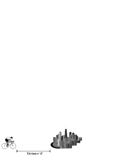
FIG. 1.: The concept of distinguishability is illustrated. What do we mean by the distance from the cyclist to the city in the figure? It is defined as the distance from the cyclist to the closest house in the city. Also, which distance measure should be chosen to appropriately measure this? In the text I argue that when it comes to distinguishing between two or more probability distributions the most appropriate measure is the relative entropy.

Sanov’s theorem. If we have a probability distribution $Q$ and a set of distributions $E\subset{\cal P}$ then

$$Q^{n}(E)\rightarrow e^{-nS(P^{*}||Q)}$$ (19)

where $P^{*}$ is the distribution in $E$ that is closest to $Q$ using the Shannon relative entropy (see Fig. 1).

This can also be rephrased in the language of distinguishability: when we are distinguishing a given distribution from a set of distributions, then what matters is how well we can distinguish that distribution from the closest one in the set (see Fig. 1). When we turn to the quantum case later, the probability distributions will become quantum densities representing various states of a quantum system, and the question will be how well we can distinguish between these states. Note that we could also talk about $Q$ coming form a set of states in which case we would have $S(P||Q^{*})$, $Q^{*}$ being the state that minimizes the relative entropy (i.e. the closest state).

B Other information measures from relative entropy

Another important concept derived from the relative entropy concerns gathering information. When one system learns something about another one, their states become correlated. How correlated they are, or how much information they have about each other, can be quantified by the mutual information.

Definition. The Shannon mutual information between two random variables $A$ and $B$, having a joint probability distribution ${p(a_{i},b_{j})}$, and therefore marginal probability distributions ${p(a_{i})}=\sum_{j}p(a_{i},b_{j})$ and ${p(b_{j})}=\sum_{i}p(a_{i},b_{j})$, is defined as

$$I_{S}(A:B):=S(p(a))+S(p(b))-S(p(a,b))\;.$$ (20)

We now present two very instructive ways of looking at this quantity, which will form a basis for the review. Mathematically, $I_{S}$ can be written in terms of the Shannon relative entropy. In this sense it represents a distance between the distribution ${p(a,b)}$ and the product of the marginals ${p(a)}\times{p(b)}$. As such, it is intuitively clear that this is a good measure of correlations, since it shows how far a joint distribution is from the product one in which all the correlations have been destroyed, or alternatively, how distinguishable a correlated state is form a completely uncorrelated one. So, we have

$$I_{S}(A:B)=S(p(a,b)\,||\,{p(a)}\times{p(b)})\;.$$ (21)

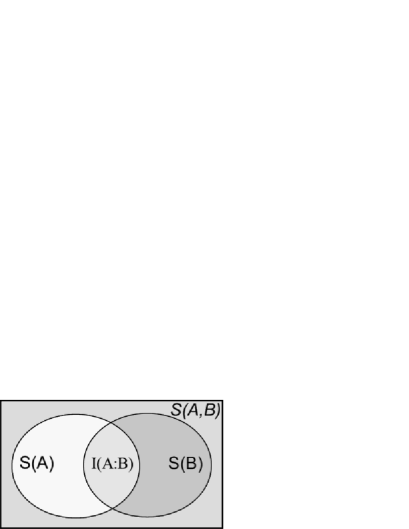
FIG. 2.: The Venn diagram representation of the joint Shannon entropy of two random variables as well as the marginal Shannon entropies. It is clear that geometrically the Shannon mutual information is obtained by summing the marginal entropies and subtracting the total entropy. It is interesting to note that its generalisation fails for three or more random variables.

Let us now view this from another angle. Suppose that we wish to know the probability of observing $b_{j}$ if $a_{i}$ has been observed. This is called a conditional probability and is given by:

$$p_{a_{i}}(b_{j}):=\frac{p(a_{i},b_{j})}{p(a_{i})}\;.$$ (22)

This motivates us to introduce a conditional entropy, $S_{A}(B)$, as:

$$S_{A}(B) = -\sum_{i}p(a_{i})\sum_{j}p_{a_{i}}(b_{j})\ln p_{a_{i}}(b_{j})$$ (23)

$$= -\sum_{ij}p(a_{i},b_{j})\ln p_{a_{i}}(b_{j})\;.$$ (24)

This quantity tells us how uncertain we are about the value of $B$ once we have learned about the value of $A$. Now the Shannon mutual information can be rewritten as

$$I_{S}(A:B)=S(B)-S_{A}(B)=S(A)-S_{B}(A)\;.$$ (25)

So, the Shannon mutual information, as its name indicates, measures the quantity of information conveyed about the random variable $A$ ($B$) through measurements of the random variable $B$ ($A$). This quantity, being positive, tells us that the initial uncertainty in $B(A)$ can in no way be increased by making observations on $A(B)$. Note also that, unlike the Shannon relative entropy, the Shannon mutual information is symmetric (see Fig. 2). The following example demonstrates the symmetry of Shannon’s mutual information.

Let us briefly go back to our original idea of a surprise to interpret the Shannon mutual information as a measure of correlations. Suppose that one of our friends likes to wear socks of two colours only: red and blue. In addition we know that her socks are always the same colour and that when she gets up in the morning, she randomly chooses the colour, but we know that she prefers blue to red with the ratio $3:1$. So, when we meet our friend, before we have looked at the colour of her socks, we know that she wears blue socks with the probability $p(b)=0.75$ and red socks with the probability $p(r)=0.25$. However, when we look at one sock and observe, say, the colour blue, we immediately know that the other sock must be blue, too. This means that the colours of her two socks are correlated. So, before we look at one of the socks, we are uncertain about the colour of the other sock by an amount of $-0.75\ln 0.75-0.25\ln 0.25$. But then, when we look at one of them the uncertainty immediately disappears. So, we expect that the information we gain about one sock by looking at the colour of the other is given by $-0.75\ln 0.75-0.25\ln 0.25$. The Shannon mutual information predicts exactly the same thing. We see that the largest correlations would be if $p(r)=p(b)=0.5$ and would be $\ln 2$. This, of course, agrees with our intuitive notion of surprise, since then, before looking at her one sock, we would be completely uncertain about the colour of the other sock. Therefore by observing its colour we obtain the largest possible amount of information (i.e. remove the largest possible uncertainty in this case).

Although it will be seen that the Shannon mutual information is a good measure of correlations between two random variables, its natural generalization to three and more random variables fails. It is easy to see that from three random variables the Shannon mutual information should be of the following form:

$$I_{S}(A:B:C) = S(A,B,C)-S(A,B)-S(A,C)-S(B,C)$$ (26)

$$+ S(A)+S(B)+S(C)\;.$$ (27)

However, there exist $A,B,C$ such that $I_{S}(A:B:C)<0$ (I leave this as an exercise for the reader), and since we regard the amount of correlation as being strictly positive, this is automatically ruled out as a good measure of correlation. A way to side-step this difficulty is to define mutual information via the relative entropy as $S(p(A,B,C)||p(A)p(B)p(C))$. This is a positive quantity representing the distance between the joint three random variables probability distribution from the product of the corresponding marginals. This, of course, immediately generalizes to any number of random variables. Next I show why the relative entropy and mutual information are also very useful from the dynamical perspective.

C Classical evolution and relative entropy

The above application of relative entropy to physics via the concept of distinguishability might seen contrived. This is, however, not at all the case, and this section shows the great importance of the relative entropy for the dynamics of classical systems. A state of a physical system in classical mechanics can be represented as a vector whose entries are various probabilities for the system to occupy its different possible states. The evolution of this system is seen as the change of these probabilities with time. So, the evolution is a linear transformation of a state into another state, i.e. of a vector into another vector,

$$q_{j}=\sum_{k}P(j|k)p_{k}$$ (28)

where $P(j|k)$ is the conditional probability for the system to change from the state $k$ to the state $j$. Because the probability has to be conserved ($\sum_{j}q_{j}=1$), we have that $\sum_{k}P(j|k)=1$. Matrices with this simple property, namely that their entries are positive and columns sum up to 1, are called stochastic. The above can be generalised to continuous systems and continuous time evolution, but this will not be relevant for the rest of this review.

A very important property of any measure that aims at quantifying the amount of correlations between two random variables (i.e two states of the same or two different systems in classical mechanics) is the following: if either or both of the variables undergo a local stochastic evolution, then the amount of correlations cannot increase (in fact, it usually decreases). We now prove this in the case of the Shannon mutual information, following an approach similar to that given by Everett (1973) (see also Penrose’s excellent book on Statistical mechanics; Penrose, 1973).

First, we establish without proof two inequalities following from the convex properties of the logarithmic functions (Everett, 1973). Lemma 1 states that entropy is a concave function, whereas lemma 2 states that the relative entropy is a convex function.

Lemma 1. $\sum_{i}P_{i}x_{i}\ln\sum_{i}P_{i}x_{i}\leq\sum_{i}P_{i}x_{i}\ln x_{i}$, where $x_{i}\geq 0$, $P_{i}\geq 0$ and $\sum_{i}P_{i}=1$.

Physically, this inequality means that the average uncertainty (negative of the right hand side) is less than or equal to the uncertainty of the average (negative of the left hand side); in other words, mixing probability distributions increases entropy. This is a very important property of entropy as a measure of uncertainty since when we mix probability distributions we expect to increase our uncertainty.

Lemma 2. $\sum_{i}x_{i}\ln\frac{\sum_{i}x_{i}}{\sum_{i}a_{i}}\leq\sum_{i}x_{i}\ln\frac{x_{i}}{a_{i}}$, where $x_{i}\geq 0$ and $a_{i}\geq 0$ for all $i$.

This is just a statement of the fact that mixing decreases distinguishability. Note that this is in accord with the lemma 1, since the more mixed the probability distributions, the less distinguishable they are.

These two simple and self-evident statements lead to a very important result that the Shannon relative entropy between two probability distributions decreases when the same two undergo a stochastic process. This is a very satisfying property from the physical point of view, where two probability distributions undergoing stochastic changes, in fact, represent two evolving physical systems. It says that two probability distributions are in some sense closer to each other (i.e. “harder to distinguish”) after a stochastic process, or analogously, that two physical systems become more alike.

So, we consider a sequence of transition-probability matrices $T^{n}_{ij}:=P_{n}(i|j)$, where $\sum_{j}T^{n}_{ij}=1$ for all $n$, $i$, and $0\leq T^{n}_{ij}\leq 1$. We also introduce a sequence of positive measures (i.e. probability distributions) $a^{n}_{i}$ having the property that

$$a^{n+1}_{j}=\sum_{i}a^{n}_{i}T^{n}_{ij}\;.$$ (29)

Transition probabilities $T$ tell us the probability that at the $n$th step of evolution the system will ”jump” from the $j$th to the $i$th state. Thus constructed transition matrices are stochastic for all $n$. We further suppose that we have a sequence of probability distributions $p^{n}_{i}$ generated by the action of the above stochastic process, such that

$$p^{n+1}_{j}=\sum_{i}p^{n}_{i}T^{n}_{ij}\;.$$ (30)

This is the law describing the systems evolution in time, and the state of the system at time $n$ is given by the probabilities $p^{n}_{i}$. For each of these probability distributions the relative entropy $S^{n}$ is defined as

$$S^{n}(p||a):=S(p^{n}||a^{n})=\sum_{i}p^{n}_{i}\ln\frac{p^{n}_{i}}{a^{n}_{i}}\;.$$ (31)

We prove the following theorem:

Distinguishability never increases.

$$S^{n+1}(p||a)\leq S^{n}(p||a).$$ (32)

Proof. Expanding $S^{n+1}(p||a)$ we obtain:

$$S^{n+1}(p||a) = \sum_{j}p^{n+1}_{j}\ln\frac{p^{n+1}_{j}}{a^{n+1}_{j}}$$ (33)

$$= \sum_{j}\{\sum_{i}p^{n}_{i}T^{n}_{ij}\}\ln\frac{\sum_{i}p^{n}_{i}T^{n}_{ij}}{\sum_{i}a^{n}_{i}T^{n}_{ij}}\,.$$ (34)

However, using lemma 2 we have the following inequality

$$\sum_{i}p^{n}_{i}T^{n}_{ij}\ln\frac{\sum_{i}p^{n}_{i}T^{n}_{ij}}{\sum_{i}a^{n}_{i}T^{n}_{ij}}\leq\sum_{i}p^{n}_{i}T^{n}_{ij}\ln\frac{p^{n}_{i}T^{n}_{ij}}{a^{n}_{i}T^{n}_{ij}}\;\;.$$ (35)

¿From the above two it follows that

$$S^{n+1}(p||a) \leq \sum_{j}\bigg{\{}\sum_{i}p^{n}_{i}T^{n}_{ij}\ln\frac{P^{n}_{i}}{a^{n}_{i}}\bigg{\}}=\sum_{i}p^{n}_{i}T^{n}_{ij}\ln\frac{p^{n}_{i}}{a^{n}_{i}}$$ (36)

$$= \sum_{i}p^{n}_{i}\ln\frac{p^{n}_{i}}{a^{n}_{i}}=S^{n}(p||a)$$ (37)

and the proof is completed _□.

This property means that a distance between two states cannot increase with time if the states evolve under any stochastic map. The proof can be immediately specialized to the cases when $T$ is stationary, i.e. $T$ is independent of $n$, and when $T$ is doubly stochastic, i.e. $\sum_{i}T_{ij}=1$ for all $j$. A corollary to this important lemma is the following:

Corollary. If we take $p=p(a,b)$, and $a=p(a)p(b)$, and suppose that the stochastic process acting separately on $A$ and $B$ are uncorrelated, we see that the Shannon mutual information does not increase under these local stochastic processes (by local we mean that they act separately on $A$ and $B$).

This is a very important, and physically intuitive, property of any measure of correlations; its quantum analogue will be of central importance for quantifying quantum correlations between entangled subsystems. This corollary, in fact, can be taken as a guidance for a “good” measure of correlations. We can state that any measure of correlations has to be non-increasing under local stochastic processes. In other words this means that the only way that the systems can become more correlated, i.e. that they gain more information about each other, is if they interact. Without mutual interaction the correlations can only decrease or at best stay the same. The nature of quantum local stochastic processes will form the physical basis for our argument in the next section. A condition similar to property above, but employing quantum stochastic processes, will be a key element in our search for measures of entanglement. When we go to quantum mechanics, the notion of a probability distribution will be replaced by a quantum state (i.e. density matrix), and a stochastic process will become a measurement process in quantum theory. The formulation of probability theory that is most naturally generalized to quantum states is provided by Kolmogorov (1950), and the quantum generalization expressing similarities with von Neumann’s Hilbert Space formulation (von Neumann, 1932) can be found in Mackey (1963) (c.f. Holevo, 1982). However, knowledge of this approach will not be necessary for the rest of the review. Finally it is important to stress that if the local stochastic processes are correlated they virtually become global, and therefore the correlations between the systems can increase as well as decrease.

D Schmidt Decomposition and Quantum Dynamics

The difference between classical and quantum physics can be seen in the fact that quantum states are described by a density matrix $\rho$ (and not just vectors). The density matrix is a positive semi-definite Hermitian matrix, whose trace is unity (representing the fact that all the probabilities add up to $1$). An important class of density matrices is the idempotent one, i.e. $\rho^{2}=\rho$. The states these matrices represent are called pure states. When there is no uncertainty in the knowledge of the state of the system its state is then pure. Another important notion is that of a composite system. A composite quantum system is one that consists of a number of quantum subsystems. When those subsystems are entangled it is impossible to ascribe a definite state vector to any one of them. The most often quoted entangled system is a pair of two photons, being in the “EPR” state (Einstein et. al, 1935; Bell, 1987). The composite system is then mathematically described by

$$|\Psi\rangle=\frac{1}{\sqrt{2}}(|\uparrow\rangle|\downarrow\rangle+|\downarrow\rangle|\uparrow\rangle)$$ (38)

where the first ket in either product belongs to one photon and the second to the other. The property that is described is the direction of spin or polarization along the z-axis, which can either be “up” ($|\uparrow\rangle$) or “down” ($|\downarrow\rangle$). A two level system of this type is a quantum analogue of a bit, which we shall henceforth call a qubit. We can immediately see that neither of the photons possesses a definite state vector. The best that one can say is that if a measurement is made on one photon, and it is found to be in the state “up” for example, then the other photon is certain to be in the state “down”. This idea cannot be applied to a general composite system, unless the former is written in a special form. This motivates us to introduce the so called Schmidt decomposition (Schmidt, 1907), which not only is mathematically convenient, but also gives a deeper insight into correlations between the two subsystems.

According to the rules of quantum mechanics the state vector of a composite system, consisting of subsystems $U$ and $V$, is represented by a vector belonging to the tensor product of the two Hilbert Spaces ${\cal H}_{U}\otimes{\cal H}_{V}$. The general state of this system can be written as a linear superposition of products of individual states:

$$|\Psi\rangle=\sum_{n}\sum_{m}c_{nm}|u_{n}\rangle|v_{m}\rangle$$ (39)

where $\{|u_{n}\rangle\}_{n=1}^{N}$ and $\{|v_{m}\rangle\}_{m=1}^{N}$ are the orthonormal basis of the subsystems $U$ and $V$ respectively, whose dimensions are dim $U=N$ and ${\em dim}V=M$. This state can always be written in the so called Schmidt form:

$$|\Psi\rangle=\sum_{n}g_{n}|u^{\prime}_{n}\rangle|v^{\prime}_{n}\rangle\;,$$ (40)

where $|u^{\prime}_{n}\rangle$ and $|v^{\prime}_{n}\rangle$ are orthonormal basis for $U$ and $V$ respectively. Note that in this form the correlations between the two subsystems are fully displayed. If $U$ is found in the state $|u^{\prime}_{2}\rangle$ for example, then the state of $V$ is $|v^{\prime}_{2}\rangle$. This is clearly a multi state generalization of the EPR state mentioned earlier.

I will now prove this assertion by showing how to derive eq. (40) from eq. (39). To that end, let us assume that $M>N$, which in no way affects our line of argument since the procedure is symmetric with respect to the subsystems. Then we have the following five steps:

1. First we construct a density matrix describing $|\Psi\rangle=\sum_{n}\sum_{m}c_{nm}|u_{n}\rangle|v_{m}\rangle$. Once the density matrix is known all the properties of the system can be deduced from it. Moreover, ensembles which are prepared differently, but have the same density matrix are statistically indistinguishable and therefore equivalent. Generally, if we have a mixed state involving vectors $|\Psi_{1}\rangle,|\Psi_{2}\rangle,\ldots|\Psi_{D}\rangle$ with corresponding classical probabilities $w_{1},w_{2},\ldots,w_{3}$, then the density matrix is defined to be:

   $$\rho=\sum_{d=1}^{D}w_{d}|\Psi_{d}\rangle\langle\Psi_{d}|\;.$$ (41)

   Since in our case $|\Psi\rangle$ is a pure state, the density matrix is a projection operator on to $|\Psi\rangle$, i.e.

   $$\rho=|\Psi\rangle\langle\Psi|=\sum_{nm}\sum_{pq}\rho_{nmpq}|u_{n}\rangle\langle u_{p}|\otimes|v_{m}\rangle\langle v_{q}|$$ (42)

   where $\rho_{nmpq}=c_{nm}c_{pq}^{*}$. If we, however, wish to deal with one of the subsystems only, then we employ the concept of the reduced density matrix.

2. We find the reduced density matrix of the subsystem $U$, obtained by tracing $\rho$ over all states of the subsystem $V$, so that

   $$\rho_{U}=\sum_{q}\langle v_{q}|\rho|v_{q}\rangle=\sum_{nm}\sum_{p}\rho_{nmpm}|u_{n}\rangle\langle u_{p}|\;.$$ (43)

   Note that the partial trace (or the trace itself) does not depend on the choice of basis. Partial tracing is analogous to finding marginal probability distributions from a joint probability distribution in classical probability theory. The crucial step in the Schmidt decomposition is diagonalizing the above. I shall call the eigenvalues of $\rho_{U}$ $|g_{1}|^{2},|g_{2}|^{2},\ldots,|g_{N}|^{2}$, and the corresponding eigenvectors $|u_{1}^{\prime}\rangle,|u_{2}^{\prime}\rangle,\ldots,|u_{N}^{\prime}\rangle$.

3. Then I re-express the above in terms of $|u^{\prime}\rangle$’s, i.e

   $$|\Psi\rangle=\sum_{n}\sum_{m}c^{\prime}_{nm}|u^{\prime}_{n}\rangle|v_{m}\rangle\;.$$ (44)

4. Now, we construct a new orthonormal basis of the subsystem $V$ such that each new vector is a “clever” linear superposition of the old ones, so that

   $$|v^{\prime}_{i}\rangle=\sum_{m}\frac{c^{\prime}_{im}}{g_{i}}|v_{m}\rangle\;.$$ (45)

   The matrix given by the coefficients $c^{\prime}_{im}/g_{i}$ is unitary which is why the new basis is orthonormal.

5. The Schmidt decomposition of $|\Psi\rangle$ is now given by

   $$|\Psi\rangle=\sum_{n}g_{n}|u^{\prime}_{n}\rangle|v^{\prime}_{n}\rangle\;.$$ (46)

There are two important observations to be made, which are fundamental to understanding correlations between the two subsystems in a joint pure state:

• The reduced density matrices of both subsystems, written in the Schmidt basis, are diagonal and have the same positive spectrum. in particular, the overall density matrix is given by

  $$\rho=\sum_{nm}g_{n}g^{*}_{m}|u^{\prime}_{n}\rangle\langle u^{\prime}_{m}|\otimes|v^{\prime}_{n}\rangle\langle v^{\prime}_{m}|$$ (47)

  whereas the reduced ones are

  $$\rho_{U} = \sum_{m}\langle v^{\prime}_{m}|\rho|v^{\prime}_{m}\rangle=\sum_{n}|g_{n}|^{2}|u^{\prime}_{n}\rangle\langle u^{\prime}_{n}|$$ (48)

  $$\rho_{V} = \sum_{n}\langle u^{\prime}_{n}|\rho|u^{\prime}_{n}\rangle=\sum_{m}|g_{m}|^{2}|v^{\prime}_{m}\rangle\langle v^{\prime}_{m}|\;.$$ (49)

• If a subsystem is $N$ dimensional it then can be entangled with no more than $N$ orthogonal states of another one.

I would like to point out that the Schmidt decomposition is, in general, impossible for more than two entangled subsystems. To clarify this I consider three entangled subsystem as an example. Here, our intention would be to write a general state such that by observing the state of the one of the subsystems we instantaneously and with certainty know the state of the other two. But, this is impossible in general, for the presence of the third system makes the prediction uncertain. Loosely speaking, while we know the state of one of the subsystems, the other two might still be entangled and cannot have definite vectors associated with them (an exception to this general rule is, for example, a state of the Greenberger–Horne–Zeilinger (GHZ) type $(1/\sqrt{2})(|\uparrow\rangle|\uparrow\rangle|\uparrow\rangle+|\downarrow\rangle|\downarrow\rangle|\downarrow\rangle)$). Clearly, involvement of even more subsystems complicates this analysis even further and produces, so to speak, an even greater mixture and uncertainty. The same reasoning applies to mixed states of two or more subsystems (i.e. states whose density operator is not idempotent $\rho^{2}\neq\rho$), for which we cannot have the Schmidt decomposition in general. This reason alone is responsible for the fact that the entanglement of two subsystems in a pure state is simple to understand and quantify, while for mixed states, or states consisting of more than two subsystems, the question is much more involved.

We now discuss the way quantum systems evolve. An isolated system, of course, follows a unitary dynamics generated by Schrödinger’s equation (non-relativistic). This evolution is fully reversible (manifesting itself in the fact that the quantum entropy does not increase during this process as we will see below). However, we know that most of the processes in Nature are irreversible (think of the spontaneous emission and the non-existence of its reverse - ”spontaneous absorption”). These processes are non-unitary and arise from the interaction of the system with the environment; thus, the system is no longer closed. Mathematically, the evolution of a quantum state is then most generally of the form (Davies, 1976)

$$\rho^{\prime}=\sum_{\alpha}A_{\alpha}\rho A^{\dagger}_{\alpha}$$ (50)

where, because of the conservation of probability, or, more precisely, trace preservation $\sum_{\alpha}A^{\dagger}_{\alpha}A_{\alpha}=1$. The above map is the most general completely positive (trace preserving) linear map (CP-map) (Choi, 1975). Positivity means that density matrices are mapped into density matrices (strictly speaking, positive operators are mapped onto positive operators). To define ”complete”, we first need to introduce the idea of an extended state. By extension of a state I mean any state on a larger Hilbert space that reduces itself to the original state when the extended part is traced out. In turn, completeness means that any extension of the density matrix is also mapped into a density matrix. To clarify this I will present a few examples of CP-maps:

• Projectors are Hermitian idempotent operators ($P^{\dagger}=P$ and $P^{2}=P$) and the evolution of the form $\rho\rightarrow\sum_{i}P_{i}\rho P_{i}$ is a CP-map;

• Addition of another system to $\rho$ is also a CP-map, $\rho\rightarrow\rho\otimes\rho_{1}$;

• Let $E_{i}\geq 0$ and $\sum_{i}E_{i}=I$. Then, $\rho\rightarrow p_{k}:=Tr(\rho E_{k})$ is a CP map which generates a probability distribution from a density matrix.

• Unitary evolution is a special case of CP-map, where only one operator is present in the sum, i.e. $U\rho U^{\dagger}$.

I leave it for the reader to show that the above CP maps can indeed be written in the form in eq. (50). We will meet other examples in the next subsection.

Remarkably not all positive maps are completely positive, transposition being a well known example. Positivity of transposition follows from the fact for any state $\rho$, its transposition $\rho^{T}\geq 0$. However, a counter example to completeness comes from, for example, a singlet state of two sub-systems $A$ and $B$. Namely, if we transpose only $A$ (or $B$), then the resulting operator is not positive (so that it is not a physical state), i.e. $\rho_{AB}^{T_{A}}<0$. Confirmation of this is left as an exercise.

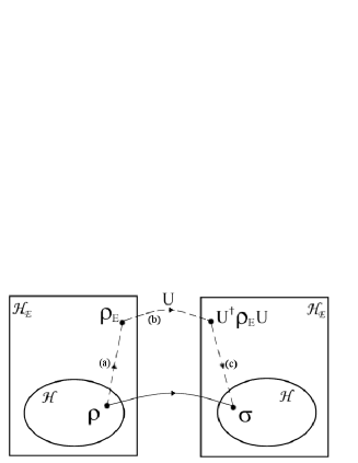
FIG. 3.: The most general evolution in quantum mechanics is represented by a completely positive trace preserving map (CP-map). This figure shows two equivalent ways of representing a CP-map: (a) the canonical form $A(.)A^{\dagger}$, and (b) via the extension to a larger Hilbert Space ${\cal H}_{E}$ and an appropriate Unitary transformation there in. The connection is explained in the text.

The reader might wonder as to what the physical implementation of the canonical form $\sum_{\alpha}A_{\alpha}\rho A^{\dagger}_{\alpha}$ is? I will now introduce another representation of the CP-maps that will explain its physical importance and will be crucial for the rest of the review. Loosely stated, any CP-map can be represented as a unitary transformation on a higher Hilbert space (see Fig. 3). Namely, from Schmidt decomposition we know that a density matrix can be represented as a ”reduction” of a state in an enlarged Hilbert space. Suppose that $\rho\in{\cal H}$ and that $\rho_{E}\in{\cal H}\otimes{\cal H}_{a}$ is an ”extension” of the state $\rho$ such that $Tr_{a}\rho_{E}=\rho$. Then a CP map $\sigma=\Phi(\rho)$ can be represented as

$$\rho\rightarrow\rho_{E}\rightarrow U\rho_{E}U^{\dagger}\rightarrow Tr_{a}(U\rho_{E}U^{\dagger})=\sigma$$ (51)

Here we have first ”lifted” $\rho$ to $\rho_{E}$, then evolved $\rho_{E}$ unitarily into $U\rho_{E}U^{\dagger}$ which, after tracing over the Hilbert space extension (i.e. lowering), yields the final state $\sigma$ as in Fig. 3. The fact that for any CP-map there exist a unitary operator $U$ which will execute this map on some higher Hilbert space is guaranteed by a theorem proved independently by Kraus (1983) and Ozawa (1984), (see Schumacher, 1996 for a modern presentation). I will now only present a plausibility argument for this correspondence. Let $\rho_{E}=\rho\otimes|0\rangle\langle 0|_{a}$ where $|0\rangle\langle 0|_{a}\in{\cal H}_{a}$. Then

$$\sigma = Tr_{a}(U\rho\otimes|0\rangle\langle 0|_{a}U^{\dagger})$$ (52)

$$= \sum_{i}\langle i|_{a}U\rho\otimes|0\rangle\langle 0|_{a}U^{\dagger}|i\rangle_{a}$$ (53)

$$= \sum_{i}\langle i|U|0\rangle\rho\langle 0|U^{\dagger}|i\rangle\;,$$ (54)

which has the same form as eq. (50) providing we define $A_{i}:=\langle i|U|0\rangle$. Thus, given a unitary evolution on the extended Hilbert Space, we can always find the corresponding positive operators which describe the evolution of the original system. Note that the choice of the operators is not unique.

Finally, I would like to discuss another frequently used concept that is in some sense derived from the notion of CP-maps. It can be loosely stated that the CP-map represents the evolution of a quantum system when we do not update the knowledge of its state based on the particular measurement outcome. This is why we have a summation over all measurements in eq. (50). If, on the other hand, we know that the outcome corresponding to the operator $A^{\dagger}_{j}A_{j}$ occurs, then the state of the system immediately afterwards is given by $A_{j}\rho A^{\dagger}_{j}/tr(A^{\dagger}_{j}A_{j}\rho)$. This type of measurement is the most general one and is commonly referred to as the Positive Operator Valued Measure (POVM). It is positive because operators of the form $A^{\dagger}A$ are always positive for any operator $A$ and taking the trace of it together with any density matrix generates a positive number (i.e. a probability for that particular measurement outcome). For a more detailed overview of POVMs see Peres (1993). The concept of POVM will play a significant role when defining the quantum relative entropy next.

E Quantum relative entropy

When two subsystems become entangled the composite state can be expressed as a superposition of the product of the corresponding Schmidt basis vectors. From eq. (40) it follows that the i-th vector of either subsystem has a probability of $|g_{i}|^{2}$ associated with it. We are, therefore, uncertain about the state of each subsystem, the uncertainty being larger if the probabilities are evenly distributed. Since the uncertainty in the probability distribution is naturally described by the Shannon entropy, this classical measure can also be applied in quantum theory. In an entangled system this entropy is related to a single observable. The general state of a quantum system, as I have already remarked, is described by its density matrix $\rho$. If $A$ is an observable pertaining to the system described by ${\rho}$, then by the spectral decomposition theorem $A=\sum_{i}a_{i}P_{i}$, where ${P}_{i}$ is the projection onto the state with the eigenvalue $a_{i}$. The probability of obtaining the eigenvalue $a_{j}$ is given by $p_{j}=\mbox{Tr}({\rho}{P}_{j})=\mbox{Tr}({P}_{j}{\rho})$. The uncertainty in a given observable can now be expressed through the Shannon entropy. Let the observables $A$ and $B$, pertaining to the subsystems $U$ and $V$ respectively, have a discrete, non-degenerate spectrum, with corresponding probabilities $p(a_{i})$ and $p(b_{j})$ of observables $A$ being $a_{i}$ and $B$ being $b_{j}$. Let also the joint probability be $p(a_{i},b_{j})$. Then,

$$S(A) = -\sum_{i}p(a_{i})\ln p(a_{i})$$ (55)

$$= -\sum_{ij}p(a_{i},b_{j})\ln\sum_{j}p(a_{i},b_{j})$$ (56)

$$S(B) = -\sum_{j}p(b_{j})\ln p(b_{j})$$ (57)

$$= -\sum_{ij}p(a_{i},b_{j})\ln\sum_{i}p(a_{i},b_{j})$$ (58)

$$S(A,B) = -\sum_{ij}p(a_{i},b_{j})\ln p(a_{i},b_{j})$$ (59)

where I have used the fact that $\sum_{j}p(a_{i},b_{j})=p(a_{i})$ and $\sum_{i}p(a_{i},b_{j})=p(b_{j})$. We have seen that a signature of correlations is that the sum of the uncertainties in the individual subsystems is greater than the uncertainty in the total state. So, the Shannon mutual information is a good indicator of how much the two given observables are correlated. However, this quantity as it is inherently classical describes the correlations between single observables only. The quantity that is related to the correlations in the overall state as a whole is the von Neumann mutual information. Since it is assigned to the state as a whole, it is of little surprise that it depends on the density matrix. First, however, I define the von Neumann entropy (von Neumann, 1932), which can be considered as the proper quantum analogue of the Shannon entropy (Ohya and Petz, 1993; Ingarden et. al, 1997; Wehrl, 1978).

Definition. The von Neumann entropy of a quantum system described by a density matrix ${\rho}$ is defined as

$$S_{N}(\rho):=-\mbox{Tr}(\rho\ln\rho)\;.$$ (60)

(I will drop the subscript $N$ whenever there is no possibility of confusion). The Shannon entropy is equal to the von Neumann entropy only when it describes the uncertainties in the values of the observables that commute with the density matrix, i.e. the Schmidt observables. Otherwise,

$$S(A)\geq S_{N}(\rho)$$ (61)

where $A$ is any observable of a system described by $\rho$. This means that there is more uncertainty in a single observable than in the whole of the state, the fact which entirely contradicts our expectations.

I now discuss a relation concerning the entropies of two subsystems. One part of it is somewhat analogous to its classical counterpart, but instead of referring to observables it is related to the two states. This inequality is called the Araki-Lieb inequality (Araki and Lieb, 1970) and is one of the most important results in the quantum theory of correlations. Let $\rho_{A}$ and $\rho_{B}$ be the reduced density matrices of subsystems $A$ and $B$ respectively, and $\rho$ be the matrix of a composite system, then:

$$S_{N}(\rho_{A})+S_{N}(\rho_{B})\geq S_{N}(\rho)\geq|S_{N}(\rho_{A})-S_{N}(\rho_{B})|\;.$$ (62)

Physically, the left hand side implies that we have more information (less uncertainty) in an entangled state than if the two states are treated separately. This arises naturally, since by treating the subsystems separately we have neglected the correlations (entanglement). We note that if the composite system is in a pure state, then $S(\rho)=0$, and from the right hand side it follows that $S(\rho_{A})=S(\rho_{B})$ (cf. Schmidt decomposition eq. (40)). To appreciate the extent to which this is a counter-intuitive result we consider the following example. Suppose a two level atom is interacting with a single mode of an EM field as in the Jaynes-Cummings model (Jaynes and Cummings, 1963). If the overall state is initially pure, and the whole system is isolated then the entropies of the atom and the field are equally uncertain at all the times. But this is not expected since the atom has only two degrees of freedom and the field infinitely many! This, however, is possible, as, by the second observation, the atom, as a two dimensional subsystem, is only entangled with two dimensions of the field.

I present without proofs two important properties of entropy which will be used in the later sections (Wehrl, 1978). These are:

$$1. \mbox{\em additivity:}\quad\,\,\,\,S_{N}({\rho}_{A}\otimes{\rho}_{B})=S_{N}({\rho}_{A})+S_{N}({\rho}_{B});$$ (63)

$$2. \mbox{\em concavity:}\quad\,\,\,\,S_{N}\left(\sum_{i}\lambda_{i}{\rho}_{i}\right)\geq\sum_{i}\lambda_{i}S_{N}({\rho}_{i});$$ (64)

The first property is the same as in classical information theory, namely the entropies of independent systems add up. The concavity simply reflects the fact that “mixing increases uncertainty”.

Following the definition of the Shannon mutual information I introduce the von Neumann mutual information, which refers to the correlation between the whole subsystems rather than relating two observables only.

Definition. The von Neumann mutual information between the two subsystems $\rho_{U}$ and $\rho_{V}$ of the joint state ${\rho}_{UV}$ is defined as

$$I_{N}(\rho_{U}:\rho_{V};\rho_{UV})=S_{N}(\rho_{U})+S_{N}(\rho_{V})-S_{N}(\rho_{UV})\;\;.$$ (65)

As in the case of the Shannon mutual information this quantity can be interpreted as a distance between two quantum states. For this I first need to define the von Neumann relative entropy, in a direct analogy with the Shannon relative entropy (in fact, this quantity was first considered by Umegaki (1962), but for consistency reasons I name it after von Neumann; I will also refer to it as the quantum relative entropy).

Definition. The von Neumann relative entropy between the two states $\sigma$ and $\rho$ is defined as

$$S_{N}(\sigma||\rho)=\mbox{Tr}\sigma(\ln\sigma-\ln\rho)\;\;.$$ (66)

This measure also has the same statistical interpretation as its classical analogue: it tells us how difficult it is to distinguish the state $\sigma$ from the state $\rho$ (Hiai and Petz, 1991). To that end, suppose we have two states $\sigma$ and $\rho$. How can we distinguish them? We can chose a POVM $\sum_{i=1}^{M}A_{i}={\bf 1}$ which generates two distributions via

$$p_{i} = trA_{i}\sigma$$ (67)

$$q_{i} = trA_{i}\rho\;\;,$$ (68)

and use classical reasoning to distinguish these two distributions. However, the choice of POVM’s is not unique. It is therefore best to choose that POVM which distinguishes the distributions most, i.e. for which the classical relative entropy is largest. Thus we arrive at the following quantity

$\displaystyle S_{1}(\sigma||\rho):=\mbox{sup}_{\mbox{A's}}\{\sum_{i}trA_{i}\sigma\ln trA_{i}\sigma-trA_{i}\sigma\ln trA_{i}\rho\},$

where the supremum is taken over all POVM’s. The above is not the most general measurement that we can make, however. In general we have $N$ copies of $\sigma$ and $\rho$ in the state

$$\sigma^{N} = \underbrace{\sigma\otimes\sigma...\otimes\sigma}_{\mbox{total of N terms}}$$ (69)

$$\rho^{N} = \underbrace{\rho\otimes\rho...\otimes\rho}_{\mbox{total of N terms}}$$ (70)

We may now apply a POVM $\sum_{i}A_{i}={\bf 1}$ acting on $\sigma^{N}$ and $\rho^{N}$. Consequently, we define a new type of relative entropy

$$S_{N}(\sigma||\rho) := \mbox{sup}_{\mbox{A's}}\{\frac{1}{N}\sum_{i}trA_{i}\sigma^{N}\ln trA_{i}\sigma^{N}$$ (71)

$$- trA_{i}\sigma^{N}\ln trA_{i}\rho^{N}\}$$ (72)

Now it can be shown that (Donald, 1986)

$$S(\sigma||\rho)\geq S_{N}$$ (73)

where $S(\sigma||\rho)$ is the quantum relative entropy. (This really is a consequence of the fact that the relative entropy does not increase under general CP-maps, a fact that will be proven later on in this subsection). Equality is achieved in eq. (73) iff $\sigma$ and $\rho$ commute (Fuchs, 1996). However, for any $\sigma$ and $\rho$ it is true that (Hiai and Petz, 1991)

$\displaystyle S(\sigma||\rho)=\lim_{N\rightarrow\infty}S_{N}\;\;.$

In fact, this limit can be achieved by projective measurements which are independent of $\sigma$ (Hayashi, 1997). From these considerations it would naturally follow that the probability of confusing two quantum states $\sigma$ and $\rho$ (after performing $N$ measurements on $\rho$) is (for large $N$):

$$P_{N}(\rho\rightarrow\sigma)=e^{-NS(\sigma||\rho)}\;\;.$$ (74)

We would like to stress here that classical statistical reasoning applied to distinguishing quantum states leads to the above formula. There are, however, other approaches. Some take eq. (74) for their starting point and then derive the rest of the formalism thenceforth (Hiai and Petz, 1991). Others, on the other hand, assume a set of axioms that are necessary to be satisfied by the quantum analogue of the relative entropy (e.g. it should reduce to the classical relative entropy if the density operators commute, i.e. if they are “classical”) and then derive eq. (74) as a consequence (Donald, 1986). In any case, as we have argued here, there is a strong reason to believe that the quantum relative entropy $S(\sigma||\rho)$ plays the same role in quantum statistics as the classical relative entropy plays in classical statistics (see also a review by Schumacher and Westmoreland, 2000).

Now, the von Neumann mutual information can be understood as a distance of the state $\rho_{UV}$ to the uncorrelated state $\rho_{U}\otimes\rho_{V}$,

$$I_{N}(\rho_{U}:\rho_{V};\rho_{UV})=S_{N}(\rho_{UV}||\rho_{U}\otimes\rho_{V})\;.$$ (75)

The quantum relative entropy will be the most important quantity in classifying and quantifying quantum correlations. It will be seen that this quantity does not increase under CP maps, which are quantum analogues of the stochastic processes. I list three properties of the relative entropy whose proof is left to the reader:

  

F1. Unitary operations leave $S(\sigma||\rho)$ invariant, i.e. $S(\sigma||\rho)=S(U\sigma U^{\dagger}||U\rho U^{\dagger})$. Unitary transformations represent a change of basis (i.e. a change in our ”perspective”) and the distance between two states should not (and does not in this case) change under this.

  

F2. $S(\mbox{Tr}_{p}\sigma||\mbox{Tr}_{p}\rho)\leq S({\sigma}||\rho)$, where $\mbox{Tr}_{p}$ is a partial trace. Tracing over a part of the system leads to a loss of information. The less information we have about two states, the harder they are to distinguish which is what this inequality says.

  

F3. The relative entropy is additive $S(\sigma_{1}\otimes\sigma_{2}||\rho_{1}\otimes\rho_{2})=S(\sigma_{1}||\rho_{1})+S(\sigma_{2}||\rho_{2})$. This inequality is a consequence of additivity of entropy itself.

These I now show have profound implication for the evolution of quantum systems.

Quantum distinguishability never increases. For any completely positive, trace preserving map $\Phi$, given by $\Phi\sigma=\sum V_{i}\sigma V^{\dagger}_{i}$ and $\sum V^{\dagger}_{i}V_{i}=1$, we have that $S(\Phi\sigma||\Phi\rho)\leq S({\sigma}||\rho)$.

I will first present a physical argument as to why we should expect this theorem to hold. As I have discussed, a CP-map can be represented as a unitary transformation on an extended Hilbert space. According to F1, unitary transformations do not change the relative entropy between two states. However, after this, we have to perform a partial tracing to go back to the original Hilbert space which, according to F2, decreases the relative entropy as some information is invariably lost during this operation. Hence the relative entropy decreases under any CP-map. I now formalise this proof.

Proof. I have discussed the fact that a CP-map can always be represented as a unitary operation+partial tracing on an extended Hilbert Space ${\cal H}\otimes{\cal H}_{n}$, where $\dim{\cal H}_{n}=n$ (Lindblad, 1974; 1975). Let $\{|i\rangle\}$ be an orthonormal basis in ${\cal H}_{n}$ and $|\alpha\rangle$ be a unit vector. So I define,

$$W=\sum_{i}V_{i}\otimes|i\rangle\langle\alpha|\,\,.$$ (76)

Then, $W^{\dagger}W=1\otimes P_{\alpha}$ where $P_{\alpha}=|\alpha\rangle\langle\alpha|$, and there is a unitary operator $U$ in ${\cal H}\otimes{\cal H}_{n}$ such that $W=U(1\otimes P_{\alpha})$ (Reed an Simon, 1980). Consequently,

$$U(A\otimes P_{\alpha})U^{\dagger}=\sum_{ij}V_{i}AV^{\dagger}_{j}\otimes|i\rangle\langle j|\,\,\,\,,$$ (77)

so that,

$$\mbox{Tr}_{2}\{U(A\otimes P_{\alpha})U^{\dagger}\}=\sum_{i}V_{i}AV^{\dagger}_{i}\,\,\,\,.$$ (78)

This shows that the unitary and $\sum_{i}V_{i}\rho V_{i}^{\dagger}$ representations are equivalent. Now using F2, then F1, and finally F3 we find the following

$$S(\mbox{Tr}_{2}\{U(\sigma\otimes P_{\alpha})U^{\dagger}\} || \mbox{Tr}_{2}\{U(\rho\otimes P_{\alpha})U^{\dagger}\})$$ (79)

$$\leq S(U(\sigma\otimes P_{\alpha})U^{\dagger}||U(\rho\otimes P_{\alpha})U^{\dagger})$$ (80)

$$= S(\sigma\otimes P_{\alpha}||\rho\otimes P_{\alpha})$$ (81)

$$= S(\sigma||\rho)\,\,\,\,.$$ (82)

This proves the result _□.

Corollary. Since for a complete set of orthonormal projectors $P$, $\sum_{i}P_{i}\sigma P_{i}$ is a CP map, then

$$\sum_{i}S(P_{i}\sigma P_{i}||P_{i}\rho P_{i})\leq S(\sigma||\rho)\,\,\,\ .$$ (83)

(The sum can be taken outside as it can be easily shown that $S(\sum_{i}P_{i}\sigma P_{i}||\sum_{i}P_{i}\rho P_{i})=\sum_{i}S(P_{i}\sigma P_{i}||P_{i}\rho P_{i})$). Now from F1, F2, F3 and eq. (83) we have the following

Theorem 5. If $\sigma_{i}=V_{i}\sigma V_{i}^{\dagger}$ then $\sum S(\sigma_{i}||\rho_{i})\leq S({\sigma}||\rho)$, where $\rho_{i}=V_{i}\rho V_{i}^{\dagger}/tr(V_{i}\rho V_{i}^{\dagger})$.

Proof. Equations (76) and (77) are introduced as in the previous proof. From eq. (77) we have that

$$\mbox{Tr}_{2}\{1\otimes P_{i}U(A\otimes P_{\alpha})U^{\dagger}1\otimes P_{i}\}=V_{i}AV^{\dagger}_{i}\,\,\,\,.$$ (84)

where $P_{i}=|i\rangle\langle i|$. Now, from F2, the Corollary and F3 it follows that

$$\sum_{i} S (\mbox{Tr}_{2}\{1\otimes P_{i}U(\sigma\otimes P_{\alpha})U^{\dagger}1\otimes P_{i}\}$$ (85)

$$|| \mbox{Tr}_{2}\{1\otimes P_{i}U(\rho\otimes P_{\alpha})U^{\dagger}1\otimes P_{i}\})$$ (86)

$$\leq \sum_{i}S(1\otimes P_{i}U(\sigma\otimes P_{\alpha})U^{\dagger}1\otimes P_{i}$$ (87)

$$|| 1\otimes P_{i}U(\rho\otimes P_{\alpha})U^{\dagger}1\otimes P_{i})$$ (88)

$$\leq S(U(\sigma\otimes P_{\alpha})U^{\dagger}||U(\rho\otimes P_{\alpha})U^{\dagger})$$ (89)

$$= S(\sigma\otimes P_{\alpha}||\rho\otimes P_{\alpha})$$ (90)

$$= S(\sigma||\rho)\,\,\,\,.$$ (91)

This proves Theorem 5 _□. This theorem will be important in the next section. A simple consequence of the fact that the quantum relative entropy itself does not increase under CP-maps is that correlations (as measured by the quantum mutual information) also cannot increase but now under local CP-maps.

Correlations cannot increase without interaction. Correlations, as measured by the von Neumann mutual information, do not increase during local complete measurements carried on two entangled quantum systems.

The Shannon mutual information, although having this desired property, does not distinguish between the quantum and classical correlations (rather, it measures total correlations). In order to do this I will have to introduce the possibility of classical communication between $A$ and $B$. This will allow classical correlations to increase while leaving quantum correlations intact, as will be seen in the following section. Now we put the theory developed so far to practical use: communication.

Digression on the Second Law of Thermodynamics. The Second Law of Thermodynamics states that entropy of an isolated system never decreases. This does not follow directly from the no increase of the quantum relative entropy under CP-maps. Strictly speaking, an isolated system in quantum mechanics evolves unitarily and therefore its entropy never changes. Under CP-maps, on the other hand, the entropy can both increase as well as decrease. If, however, the state $\rho$ is maximally mixed $I/n$ for example, then the quantum relative entropy is given by:

$$S(\sigma||\rho)=\ln n-S(\sigma)\;.\noindent$$ (92)

If in addition the evolution is such that $I/n$ is the equilibrium state, then the monotone decrease in the quantum relative entropy implies a monotone increase in $S(\sigma)$, just as in the Second Law of Thermodynamics. Otherwise, the entropy itself can both increase as well as decrease. A detailed discussion of the statistical foundations of the Second Law can be found in Tollman’s classic ”The Principles of Statistical Mechanics” (Tolman, 1938).

III Quantum communication: Classical Use

The central objective of communication theory is to allow a person, often referred to as Alice, to communicate accurately with another person, called Bob, even in the presence of noise. Alice encodes her message into a number of different (distinguishable) states, with each state representing a different symbol in the message. For example, Alice encodes the bit value $1$ into the excited state of a two level atom and sends this atom to Bob. On its way to Bob the atom may transform into its ground state due to either stimulated or spontaneous emission thereby giving Bob the impression that Alice transmitted $0$. This unwanted state transition is a form of channel noise.

The key question is: what is the largest amount of information (per symbol) that Alice can send to Bob, i.e. what is the capacity of the communication channel taking into account any possible noise? In classical information theory the capacity for communication is given by the mutual information between Alice’s sent message and Bob’s received message (Shannon and Weaver, 1949). This is intuitively clear, since mutual information quantifies correlations between sent and received messages and it thus tells us how faithful the transmission is. If we use quantum states to encode symbols, then the capacity is not given by the quantum mutual information we introduced before. We derive a new quantity for this purpose called the Holevo bound (Holevo, 1973). The benefit of performing the full quantum derivation is that this is a more fundamental approach to information processing. We can then deduce the classical capacity as a special case.

A Holevo bound

A quantum communication channel (QCC) consists of a number, $N$, of quantum systems prepared in states $\rho_{1},\rho_{2}\ldots\rho_{N}$ and whatever physical medium is used to send the states from Alice to Bob. These states encode $N$ different symbols with certain a priori probabilities, $p_{1},p_{2},\ldots p_{N}$. Bob then performs a set of measurements to determine the correct sequence of states comprising Alice’s symbols, which he can then use to reconstruct the entire message (Ingarden, 1976). If the states suffer no error on the way to the Bob, then the channel is called noiseless; otherwise it is called noisy. I only consider the notion of capacity of a noiseless QCC, since the generalization to a noisy channel is straightforward.

Let $S(\rho)=-\mbox{Tr}\rho\ln\rho$ be the standard von Neumann entropy of a density matrix $\rho$. Then, the capacity of a QCC is defined as

$${\bf C}:=\max_{\{p\}}C(\{p\},\rho)$$ (93)

where

$$C(\{p\},\rho)=S(\sum_{i}p_{i}\rho_{i})-\sum_{i}p_{i}S(\rho_{i})\;\;,$$ (94)

is the Holevo bound. Note that the above can be expressed succinctly as

$$C(\{p\},\rho)=\sum_{i}p_{i}S(\rho_{i}||\rho)\;\;,$$ (95)

where $S(\;||\;)$ is the von Neumann relative entropy and $\rho=\sum_{i}p_{i}\rho_{i}$. When there is no possibility of confusion I write $C(\{p\},\rho)\equiv C(\{p\})$. The reader may ask why we need to maximise symbol probabilities in order to compute the capacity. This is because the channel can be used with different input probabilities and the capacity represents the maximum that can be communicated using this channel.

To see the physical motivation behind this quantity consider $N$ states $\rho_{1},...\rho_{N}$ sent by Alice to Bob according to probabilities $p_{1},...p_{N}$ respectively. Bob now performs a set of complete measurements $\sum_{i}E_{i}=I$, where $E_{i}\geq 0$, in order to determine which state was sent to him (a complete measurement is like a CP-map, but where we record each of the outcomes). The accessible information to Bob is given by the mutual information between his measurement and $\rho_{1},...\rho_{N}$ (Holevo, 1973; Davies 1976). This quantity tells us how well Bob’s measurement can distinguish between the message states and is given by

$$I(E:\rho) = \bigg{\{}\sum_{i}-\mbox{Tr}(\rho E_{i})\ln(\mbox{Tr}(\rho E_{i}))$$ (96)

$$+ \sum_{j}p_{j}\mbox{Tr}(\rho_{j}E_{i})\ln(\mbox{Tr}(\rho_{j}E_{i}))\bigg{\}}$$ (97)

The rationale behind this expression is that the uncertainty in the message before any measurement is performed is given by the first term and the second term represents the uncertainty after the measurement has identified (partially in general) the message states. The Holevo bound is an upper bound to the above accessible information, i.e.

$$S(\sum_{i}p_{i}\rho_{i})-\sum_{i}p_{i}S(\rho_{i})\geq\max_{E}I(E:\rho)\;.$$ (98)

This equality is saturated if and only if $[\rho_{i},\rho_{j}]=0$ for all $i$ and $j$. Therefore, since the Holevo bound is an upper bound to accessible information that Bob can gain about Alice’s message, we identify its maximum over all possible initial probabilities with the classical capacity of a quantum channel.

The Holevo bound has an even more suggestive form: the uncertainty in the initial message is $S(\rho)$, but after the states are correctly identified the average uncertainty is $\sum_{i}p_{i}S(\rho_{i})$. The difference between these two quantities when maximised over all $p_{i}$s is the classical communication capacity of a quantum channel. Note that one of the most profound implications of the Holevo bound is that a quantum bit cannot store more information than a classical bit. In spite of this limitation, quantum information processing is more efficient than its classical analogue. This is due to the different nature of information encoding, which is reflected in the existence of superpositions of different states as well as entanglement between different qubits (see also section on dense coding).

Proof of the Holevo bound in eq. (98). The Holevo bound is a direct consequence of the fact that the quantum relative entropy does not increase under CP maps as in Theorem 1 (note that Holevo’s original proof is much more complicated and does not involve using the quantum relative entropy. Here I follow Yuen and Ozawa in spirit, as in the last reference of Holevo (1973)). One such map is

$$\tau(A)=\frac{1}{n}\mbox{Tr}(A)$$ (99)

where $A$ is any $n\times n$ positive matrix. This leads to the Pierls - Bogoliubov inequality (PBI) (Bhatia, 1997)

$$\tau(A)(\ln\tau(A)-\ln\tau(B))\leq\tau(A\ln A-A\ln B)$$ (100)

To prove the Holevo bound I first use that fact that (Theorem 5)

$$S(\rho_{i}||\rho)\geq\sum_{j}S(A_{j}\rho_{i}A^{\dagger}_{j}||A_{j}\rho A^{\dagger}_{j})$$ (101)

PBI now implies that

$$S(A_{j}\rho_{i}A^{\dagger}_{j}||A_{j}\rho A^{\dagger}_{j}) \geq \mbox{Tr}(A_{j}\rho_{i}A^{\dagger}_{j})\{\ln(\mbox{Tr}(A_{j}\rho_{i}A^{\dagger}_{j}))$$ (102)

$$- \ln(\mbox{Tr}(A_{j}\rho A^{\dagger}_{j}))\}$$ (103)

$$= p(j|i)(\ln p(j|i)-\ln p(j))$$ (104)

where $p(j|i)=Tr\{A_{j}\rho_{i}A^{\dagger}_{j}\}$ is the conditional probability that the message $\rho_{i}$ will lead to the outcome $E_{j}=A^{\dagger}_{j}A_{j}$ and $p(j)=\sum_{i}p(j|i)$. Thus we now have that

$$S(\rho_{i}||\rho)\geq\sum_{j}p(j|i)(\ln p(j|i)-\ln p(j))$$ (105)

Multiplying both sides by the (positive) $p_{i}$ and summing over all $i$ leads to the Holevo bound _□.

Since Holevo’s result is one of the key results in quantum information theory I present another simple way of understanding it via the quantum mutual information. This, of course, is only an additional motivation for the Holevo bound and by no means proves its validity. Namely, if Alice encodes the symbol (sym) $i$ into the state (st) $\rho_{i}$, then the total state (sym $+$ st) is

$$\rho_{Sym+St}=\sum_{i}p_{i}|i\rangle\langle i|\otimes\rho_{i}\;,$$ (106)

where the kets $|i\rangle$ are orthogonal (we can think of these as representing different states of consciousness of Alice!). Bob now wants to learn about the symbols by distinguishing the states $\rho_{i}$. He cannot learn more about the symbols than is already stored in the correlations between the symbols and the message states. This as we know is given by the quantum mutual information

$$I(\rho_{Sym+St}) = S(Sym)+S(St)-S(Sym+St)$$ (107)

$$= S(\sum_{i}p_{i}\rho_{i})-\sum_{i}p_{i}S(\rho_{i})$$ (108)

which is the same as the Holevo bound.

I would like now to derive the capacity of a classical communication channel from the Holevo bound. I follow Gordon’s reasoning who was, in fact, the first person to conjecture the Holevo bound (Gordon, 1964). As I mentioned before, the Holevo bound itself contains the classical capacity of a classical channel as a special case. This, as we might expect, happens when all $\rho_{i}$s are diagonal in the same basis, i.e. they commute (classically all the states and observables commute because they can be simultaneously specified and measured which is in contrast with quantum mechanics). Therefore density matrices are reduced to classical probability distributions. Let us call this basis the $B$ representation, with orthonormal eigenvectors $|b\rangle$. Then the probability that the measurement of the symbol represented by $\rho_{i}$ will yield the value $b$ is just $\langle b|\rho_{i}|b\rangle$. This I call the conditional probability $p_{i}(b)$, that if $\rho_{i}$ was sent the result $b$ was obtained. Now the Holevo bound is

$${\bf C}=S(\rho)-\sum_{i}p_{i}S(\rho_{i})=S(\rho)-S_{B}(\rho_{i})\;,$$ (109)

where $S_{B}(\rho_{i})$ is the conditional entropy given by

$$S_{B}(\rho_{i})=\sum_{i}p_{i}\sum_{b}\langle b|\rho_{i}|b\rangle\ln\langle b|\rho_{i}|b\rangle=\sum_{i}p_{i}S(\rho_{i})\;.$$ (110)

Thus, the Holevo bound reduces itself to the Shannon mutual information between the commuting messages and the measurement in the B representation.

In general, the usual rule of thumb for obtaining quantum information theoretic quantities from their classical counter-parts is by the convention

$$\sum \longrightarrow\mbox{Trace}$$ (111)

$$\sum p(a) \longrightarrow\rho_{A}\;,$$ (112)

so that, for example, the Shannon entropy $S(p(a))=-\sum_{i}p(a_{i})\ln p(a_{i})$ now becomes the von Neumann entropy $S(\rho_{A})=-\mbox{Tr}\rho_{A}\ln\rho_{A}$.

Example. As the first application of the Holevo bound I will compute the channel capacity of a Bosonic field, e.g. Electromagnetic field (for an excellent review see Caves and Drummond, 1994). The message information will now be encoded into modes of frequency $\omega$ and average photon number $\bar{m}(\omega)$. The signal power is assumed be $S$. The noise in the channel is quantified by the average number of excitations $\bar{n}(\omega)$ and is assumed to be independent of the signal (i.e. the power of signal and noise is additive). We saw that when there is no noise in the channel the Holevo bound is equal to the entropy of the average signal. In order to compute the capacity we need to maximize this entropy with the constraint that the total power (or energy) is fixed. It is well known that thermal states are those that maximize the entropy. We thus assume that both the noise and signal+noise are in thermal equilibrium and follow the usual Bose-Einstein statistics. The noise power is

$$N=\frac{\pi(kT)^{2}}{12\hbar}$$ (113)

The power of the output of the channel (signal+noise) is

$$P=S+N=\frac{\pi(kT_{e})^{2}}{12\hbar}$$ (114)

where $T_{e}$ is the equilibrium temperature of signal+noise. Therefore it follows that

$$T_{e}=(12\hbar S/\pi k^{2}+T^{2})^{1/2}$$ (115)

The state of the noise in the mode $\omega$ is

$$\rho_{N}(\omega)=\sum_{n}\frac{1-e^{-\hbar\omega/kT}}{e^{\bar{n}(\omega)\hbar\omega/kT}}|n\rangle\langle n|$$ (116)

while the state of the output is

$$\rho_{N+S}(\omega)=\sum_{n}\frac{1-e^{-\hbar\omega/kT_{e}}}{e^{\bar{n}(\omega)\hbar\omega/kT_{e}}}|n\rangle\langle n|$$ (117)

The capacity of the channel is given by the Holevo bound which is

$$C = \int_{-\infty}^{\infty}[S(\rho_{S+N}(\omega))-S(\rho_{N}(\omega))]d\omega$$ (118)

$$= \frac{\pi kT}{6\hbar\ln 2}\{(12\hbar S/\pi(kT)^{2}+1)^{1/2}-1\}$$ (119)

The integration is there to take into account all the modes of the field. Let us look at the two extreme limits of this capacity. In the high temperature limit we obtain the ”classical” capacity

$$C_{C}=\frac{S}{kT\ln 2}\;,$$ (120)

a result derived by Shannon and Weaver (1949). This states that in order to communicate one bit of information with this set-up we need exactly $kT\ln 2$ amount of energy. In the low temperature limit, on the other hand, quantum effects become important and the capacity becomes independent of $T$

$$C_{Q}=\frac{\sqrt{\pi}}{\ln 2}\{\frac{S}{\hbar}\}^{1/2}\;,$$ (121)

which was derived by Stern (1960), Gordon (1964), Lebedev and Levitin (1963) and Yamamoto and Haus (1986) among others. Note also the appearance of Planck’s constant which is a key feature of quantum mechanics. If we wish to communicate one bit of information in this limit we need only $\hbar/\pi(\ln 2)\sim 10^{-34}$ joules of energy. This is significantly less than the corresponding energy in the classical limit. Let us now compare the classical and quantum capacity limits to the total energy of $N$ harmonic oscillators (Bosons) in the same two limits. In the high temperature limit the equipartition theorem is applicable and the total energy is $3NkT$ (i.e. it depends on temperature). In the low temperature limit all the Harmonic oscillators settle down to the ground state so that the total energy becomes $N\hbar\omega/2$ (i.e. it is independent of temperature and we see the quantum dependence through Plank’s constant $\hbar$).

B Schumacher’s compression

The most optimal communication through a noiseless channel using pure states is equivalent to data compression. We have seen in eq. (15) that the limit to the classical data compression is just given by the entropy of the probability distribution of the data. We would thus guess that the limit to quantum data compression is given by the von Neumann entropy of the set of states being compressed. This, in fact, turns out to be a correct guess as first proven by Schumacher (1995). So, Alice now encodes letters of her classical message into pure quantum states and sends these to Bob. For example if $a\rightarrow|\psi_{a}\rangle$ and $b\rightarrow|\psi_{b}\rangle$, then Alice’s message $aab$ will be sent to Bob as the sequence of pure quantum states $|\psi_{a}\rangle|\psi_{a}\rangle|\psi_{b}\rangle$.

The exact problem can be phrased in the following equivalent fashion: suppose a quantum source randomly prepares different qubit states $|\psi_{i}\rangle$ with the corresponding probabilities $p_{i}$. A random sequence of $n$ such states is produced. By how much can this be compressed, i.e. how many qubits do we really need to encode the original sequence (in the limit of large $n$)? First of all the total density matrix is

$$\rho=\sum_{i}p_{i}|\psi_{i}\rangle\langle\psi_{i}|$$ (122)

Now, this matrix can be diagonalised

$$\rho=\sum_{i}r_{i}|r_{i}\rangle\langle r_{i}|$$ (123)

where $r_{i}$ and $|r_{i}\rangle$ are the eigenvectors and eigenvalues. This decomposition is, of course, indistinguishable from the original one (or any other decomposition for that matter). Thus we can think about compression in this new basis, which is easier as it behaves completely classically (since $\langle r_{i}|r_{i}\rangle=\delta_{ij}$). We can therefore invoke results from the previous section on classical typical sequences and conclude that the limit to compression is $n(-\sum_{i}r_{i}\ln r_{i})$, i.e. $n$ qubits can be encoded into $nS(\rho)$ qubits. No matter how the states are generated, as long as the total state is described by the same density matrix $\rho$ its compression limit is its von Neumann entropy. This protocol and result will be very important when we discuss entanglement measures in the following section.

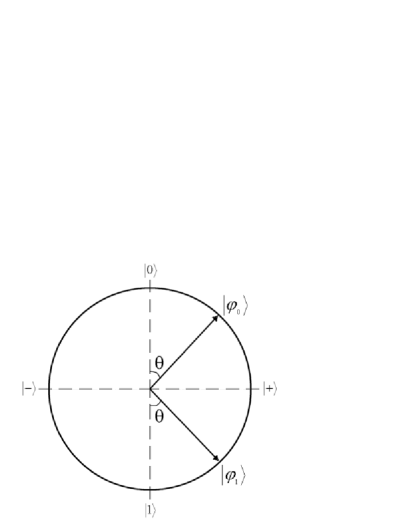
FIG. 4.: This figure shows the two non-orthogonal states on the Bloch sphere which are used to encode a message. The overlap between them is $\sin\theta$ and the smaller the overlap, the more the total message can be compressed. In terms of information, the less distinguishable the states (i.e. the smaller the overlap), the less information they carry.

Example. Suppose that Alice encodes her bit into states $|\Psi_{0}\rangle=\cos(\theta/2)|0\rangle+\sin(\theta/2)|1\rangle$ and $|\Psi_{1}\rangle=\sin(\theta/2)|0\rangle+\cos(\theta/2)|1\rangle$ with $p_{0}=p_{1}=1/2$ (see Fig. 4). Classically it is not possible to compress a source that generates $0$ and $1$ with equal probability. Quantum mechanically, however, compression can be achieved not only by the nature of the probability distribution but also due to the non-orthogonality of the states encoding symbols of the message. In our example the overlap between the two states is $\langle\psi_{0}|\psi_{1}\rangle=sin\theta$ and they are orthogonal only when $\theta=\pi$ in which case no compression is possible. Otherwise, the compression ratio is directly proportional to the overlap between the states. Suppose Alice’s messages are only $3$ qubits long. Then there are $8$ different possibilities, $|\Psi_{0}\Psi_{0}\Psi_{0}\rangle,...|\Psi_{1}\Psi_{1}\Psi_{1}\rangle$, which are all equally likely with $1/8$ probability. In general these states will lie with a high probability within a subspace of the $8$ dimensional Hilbert space. Let us call this likely subspace a ”typical” subspace. Its orthogonal complement will be unlikely and hence called an ”atypical” subspace. In order to find the typical and atypical subspaces we need to diagonalise the ”average” signal

$$\rho=\frac{1}{2}(|\Psi_{0}\rangle\langle\psi_{0}|+|\Psi_{1}\rangle\langle\psi_{1}|)$$ (124)

Its diagonal form is

$$\rho=\frac{1}{2}(1+\sin\theta)|+\rangle\langle+|+\frac{1}{2}(1-\sin\theta)|-\rangle\langle-|$$ (125)

where $|\pm\rangle=|0\rangle\pm|1\rangle$. Now we look at the probabilities for each of the $8$ messages to lie along the new orthogonal basis $|+++\rangle,...|---\rangle$ of the Hilbert space of three qubits:

$$|\langle+++|\psi^{\otimes 3}\rangle|^{2} = (\cos(\theta/2)+\sin(\theta/2))^{6}$$ (126)

$$|\langle++-|\psi^{\otimes 3}\rangle|^{2} = (\cos(\theta/2)+\sin(\theta/2))^{4}$$ (127)

$$+ (\cos(\theta/2)-\sin(\theta/2))^{2}$$ (128)

$$|\langle+--|\psi^{\otimes 3}\rangle|^{2} = (\cos(\theta/2)+\sin(\theta/2))^{2}$$ (129)

$$+ (\cos(\theta/2)-\sin(\theta/2))^{4}$$ (130)

$$|\langle---|\psi^{\otimes 3}\rangle|^{2} = (\cos(\theta/2)-\sin(\theta/2))^{6}\;$$ (131)

where $|\psi^{\otimes 3}\rangle$ represents any $3$ qubit sequence of $|\psi_{0}\rangle$ and $|\psi_{1}\rangle$. In addition all the probabilities for $|++-\rangle,|+-+\rangle,|-++\rangle$ are equal and so are the probabilities for $|+--\rangle,|--+\rangle,|-+-\rangle$. Thus the above equation contains $64$ probabilities in total. Suppose now that $\cos(\theta/2)\sim\sin(\theta/2)$. Then, we see that the states containing two or more $+$ become much more likely. This means that the message states are much more likely to be in this particular subspace. Therefore the compression would be as follows. First the source generates three qubits in some state. Then we project this message onto the typical subspace. If we are successful, then this will lie in that four dimensional typical subspace for which we need only two qubits rather than three. Otherwise, our projection will fail and the message will end up in the atypical subspace in which case Alice does not compress it. The probability to end up in the atypical space asymptotically goes to zero (the law of large numbers). Therefore in this example the limit to our compression is given by $-(1/2(1+\sin\theta))\ln(1/2(1+\sin\theta))-(1/2(1-\sin\theta))\ln(1/2(1-\sin\theta))$ which is of course the von Neumann entropy of $\rho$. The number of dimensions of the typical subspace of the total Hilbert space is likewise in general equal to $e^{nS(\rho)}$.

Interestingly, if instead of pure states a quantum source generates mixed states $\rho_{i}$ with probabilities $p_{i}$, then the best compression limit is in general unknown. We can, of course, use the above protocol to compress the sequence to the von Neumann entropy of the average signal, $S(\sum_{i}p_{i}\rho_{i})$. However, in some cases it is known that a better compression can be achieved. The lower bound to compression is the Holevo bound, $S(\sum_{i}p_{i}\rho_{i})-\sum_{i}p_{i}S(\rho_{i})$, but it is not known whether this bound can in general be attained (see Horodecki, 1998b).

Next we look at a protocol for classical communication that involves entanglement. At first sight this protocol seems to violate the Holevo bound on classical communication, i.e. that it is possible to communicate only 1 bit per single qubit. However, a closer inspection will show that this is not the case.

C Dense coding

Now I consider the case of dense coding which was introduced by Bennett and Wiesner, 1992. In this protocol entanglement plays a crucial role and this will give us a first indication of the fact that entanglement can be quantified like any other resource, such as energy for example. Alice and Bob initially share an entangled pair of qubits in some state $W_{0}$, which may be mixed. Alice then performs local unitary operations on her qubit to put this shared pair of qubits into either of the states $W_{0},W_{1},W_{2}$ or $W_{3}$. In general, Alice may use a completely arbitrary set of unitary operations to generate these states:

$$W_{i}={\bf U_{i}}\otimes{\bf I}~{}W_{0}~{}{\bf U_{i}^{\dagger}}\otimes{\bf I},$$ (132)

and the number of generated states is completely arbitrary. In the above equation, ${\bf U_{i}}$ acts on Alice’s qubit and ${\bf I}$ acts on Bob’s qubit. By sending her encoded qubit to Bob, Alice is essentially communicating with Bob using the states $W_{0},W_{1},W_{2}$ and $W_{3}$ as separate letters. The number of bits she can communicate to Bob using this procedure is thus bounded by the Holevo bound. Moreover, if some block coding is done on a large enough collection of qubits in addition to the dense coding, then the number of bits of information communicated is equal to the Holevo function. We will thus take

$$\mbox{\bf C}=S(\rho)-\sum_{i}p_{i}S(\rho_{i}),$$ (133)

assuming that any additional necessary block coding will automatically be performed to supplement the dense coding. This coding is essential in order to achieve the capacity given by the Holevo bound, in the asymptotic limit (The fact that the bound is achievable follows from a complicated argument and cannot really be derived using the arguments presented in this review. Hausladen et. al (1996) have proved this for pure states and Schumacher and Westmoreland (1997) and independently Holevo (1998) for mixed states). Exactly the same assumption has been used in Ref. Hausladen et. al (1996) to calculate the capacity for dense coding in the case of pure letter states. Eqs.(132) and (133) define the most general version of dense coding and I shall refer to this as completely general dense coding (CGCD).

A simpler example of dense coding is the case when the letter states are generated from the initial shared state $W_{0}$ by

$$W_{0}={\bf I}\otimes{\bf I}~{}W_{0}~{}{\bf I}\otimes{\bf I},$$ (134)

$$W_{1}={\bf\sigma_{1}}\otimes{\bf I}~{}W_{0}~{}{\bf\sigma_{1}}\otimes{\bf I},$$ (135)

$$W_{2}={\bf\sigma_{2}}\otimes{\bf I}~{}W_{0}~{}{\bf\sigma_{2}}\otimes{\bf I},$$ (136)

$$W_{3}={\bf\sigma_{3}}\otimes{\bf I}~{}W_{0}~{}{\bf\sigma_{3}}\otimes{\bf I}.$$ (137)

In the above set of equations, the first operator of the combination ${\bf\sigma_{i}}\otimes{\bf I}$ acts on Alice’s qubit and the second operator acts on Bob’s qubit. I shall refer to this case (i.e when the letter states are generated by Eqs.(134)-(137)) as simply general dense coding (GDC). The generality present in GDC is that Alice is allowed to prepare the different letter states with unequal probabilities.

In the more special case when Alice not only generates the four letter states according to Eqs.(134)-(137)) but also with equal probability, the ensemble is given by

$$W=\frac{1}{4}\sum_{i=0}^{3}W_{i}.$$ (138)

and the capacity becomes

$$\mbox{\bf C}=\frac{1}{4}\sum_{i=0}^{3}S(W_{i}||W).$$ (139)

I shall call this simplest case special dense coding (SDC). Among all the possible ways of doing GDC, SDC is the optimal way to communicate when $W_{0}$ is a pure state (Bose et. al 2000a) or a Bell diagonal state.

Now I derive the most general bound on CGDC (Bowen, 2001). Furthermore, this bound can be attained by the same protocol as SDC (Bowen, 2001). The proof is achieved by first finding an upper bound to the capacity for CGDC and then showing that SDC actually saturates this bound. Suppose that the initial state of Alice and Bob is $\rho_{AB}$. Then we have:

C $$= \max S(\sum_{k}p_{k}(U^{k}\otimes I)\rho_{AB}((U^{k})^{\dagger}\otimes I))$$ (140)

$$- \sum_{k}p_{k}S((U^{k}\otimes I)\rho_{AB}((U^{k})^{\dagger}\otimes I))$$ (141)

$$= \max S(\rho^{\prime}_{AB})-S(\rho_{AB})$$ (142)

$$\leq S(\rho^{\prime}_{A})+S(\rho^{\prime}_{B})-S(\rho_{AB})$$ (143)

$$\leq 1+S(\rho_{B})-S(\rho_{AB})$$ (144)

Since this bound is achievable as shown by Bowen (2001), the capacity for CGDC is given by eq. (144).

I shall now restrict my attention to a calculation of ${\bf C}$ for pure letter states. Consider the initial shared pure state $W_{0}$ to be,

$$|\psi_{0}\rangle=(a|00\rangle+b|11\rangle).$$ (145)

Then, according to Eqs.(134)-(137), the other letter states are given by

$$|\psi_{1}\rangle=(a|10\rangle+b|01\rangle),$$ (146)

$$|\psi_{2}\rangle=-i(a|10\rangle-b|01\rangle),$$ (147)

$$|\psi_{3}\rangle=(a|00\rangle-b|11\rangle),$$ (148)

from which we obtain $W_{i}=|\psi_{i}\rangle\langle\psi_{i}|$. As all $W_{i}$ are pure states we have

$$S(W_{i})=0.$$ (149)

Thus we have

$$\mbox{\bf C}=S(W).$$ (150)

I will consider only the case of SDC as it is optimal. Thus the ensemble used is obtained from Eq.(138) to be

$$W = \frac{|a|^{2}}{2}|00\rangle\langle 00|+\frac{|b|^{2}}{2}|01\rangle\langle 01|$$ (151)

$$+ \frac{|a|^{2}}{2}|10\rangle\langle 10|+\frac{|b|^{2}}{2}|11\rangle\langle 11|.$$ (152)

Thus from Eq.(150) for the capacity C, we get

C $$= -(|a|^{2}\log\frac{|a|^{2}}{2}+|b|^{2}\log\frac{|b|^{2}}{2})$$ (153)

$$= 1-(|a|^{2}\log|a|^{2}+|b|^{2}\log|b|^{2}).$$ (154)

(Note that this agrees with eq. (144) as for pure states the total entropy is zero.) Now this implies that a good measure of entanglement for a pure state of a system composed of two subsystems A and B can be given by the von Neumann entropy of the state of either of the subsystems. Let us call this measure the von Neumann entropy of entanglement and label it by $E_{v}$ (Popescu and Rohrlich, 1997; Bennett et. al, 1996a). Thus

$$E_{v}(|\psi\rangle\langle\psi|_{\mbox{}{A+B}})=S{(}\mbox{Tr}_{\mbox{}{A}}(|\psi\rangle\langle\psi|_{\mbox{}{A+B}}){)},$$ (155)

where $\mbox{Tr}_{\mbox{}{A}}$ stands for partial trace over states of system A. Therefore, for all the states $W_{i}$,

$$E_{v}(W_{i})=-(|a|^{2}\log|a|^{2}+|b|^{2}\log|b|^{2}).$$ (156)

Thus,

$$\mbox{\bf C}=1+E_{v}(W_{i}).$$ (157)

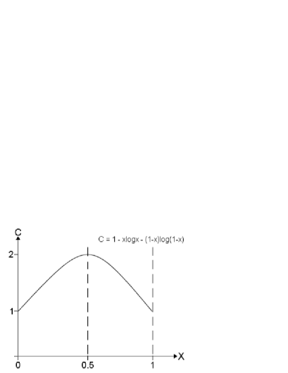
FIG. 5.: This figure shows the dependence of capacity for dense coding for pure states $a|00\rangle+b|11\rangle$ as a function of its Schmidt coefficient $x=|a|^{2}$. We see that when the state is disentangled, i.e. when either $a=0$ or $b=0$, the capacity becomes 1 bit per qubit, i.e. the same as the ”classical capacity”.

(see Fig. 5). We can prove that for pure states, SDC (using all alphabet states with equal a priori probability) is the optimal way to communicate among all possible ways of doing GDC (i.e when the letter states are generated by Eqs.((134)-(137)) (Bose et. al, 2000a). Important, however, is the fact that the amount of entanglement determines exactly how much information Alice can convey to Bob. Note that if there is no entanglement shared between them, then the amount of information is exactly one bit per Alice’s qubit (which is what can be achieved classically after all). At the other extreme, when they share a maximally entangled state, the amount of information is $2$ bits per Alice’s qubit. This is the amount that no purely classical communication can achieve. However, while the von Neumann entropy is a good measure of entanglement for pure states (in fact, there are arguments that it is unique for pure states (Popescu and Rohrlich, 1997)), it fails when we try to apply it to mixed states. A possibility is to follow the logic of the pure state dense coding and call $S(\rho_{B})-S(\rho_{AB})$ a measure of entanglement for mixed states as in eq. (144). This measure has been called the “coherent information” and is used to describe information transmission through a noisy quantum channel, as in e.g. Barnum et.al (1998). But, is this measure consistent with other natural requirements for quantifying entanglement? This question will be addressed in the next section. Before this, we show that in order to delete a certain amount of correlations we need to increase the entropy of the environment by at least this amount. This is known as Landauer’s erasure (Landauer, 1961) and is seen to be linked directly to the relative entropy.

D Relative entropy, thermodynamics and information erasure

We have seen that communication essentially creates correlations between the sender and the receiver. Creating correlations is therefore very important in order to be able to convey any information. However, I would now like to talk about the opposite process - deleting correlations. Why would one want to do so? The reason is that we might want to correlate one system to another and may need to delete all its previous correlations to be able to store new ones. I would like to give a more physical statement of information erasure and link it to the notion of measurement. I will therefore introduce two correlated parties - a system and an apparatus. The apparatus will interact with the system thereby gaining a certain amount of information about it (the full quantum description of this process will be presented in section V). Suppose now that the apparatus needs to measure another system. We first need to delete information about the last system before we can make another measurement. The most general way of conducting erasure (resetting) of the apparatus is by employing a reservoir in thermal equilibrium at certain temperature $T$. To erase the state of the apparatus we just throw it into the reservoir and introduce a new pure state. The entropy increase of the operation now consists of two parts. Firstly, the state of the apparatus evolves to the state of the reservoir and this entropy is now added to the reservoir entropy. Secondly, the rest of the reservoir changes its entropy due to this interaction which is the difference in the apparatus internal energy before and after the resetting (no work is done in this process). This quantum approach to equilibrium was also studied by Partovi (1989). A good model is obtained by imagining that the reservoir consists of a great number of systems (of the same ”size” as the apparatus) all in the same quantum equilibrium state $\omega$. Then the apparatus, which is in some state $\rho$, interacts with these reservoir systems one at a time. Each time there is an interaction, the state of the apparatus approaches more closely the state of the reservoir, while that single reservoir system also changes its state away from the equilibrium. However, the systems in the bath are numerous so that after a certain number of collisions the apparatus state will approach the state of the reservoir, while the reservoir will not change much since it is very large (this is equivalent to the so called Born-Markov approximation that leads to irreversible dynamics of the apparatus described here).

Bearing all this in mind, we now reset the apparatus by plunging it into a reservoir in a thermal equilibrium (Gibbs state) at temperature $T.$ Let the state of the reservoir be

$\displaystyle\omega=\frac{e^{-\beta H}}{Z}=\sum_{j}q_{j}\left|\varepsilon_{j}\right\rangle\left\langle\varepsilon_{j}\right|$

where $H=$ $\sum_{i}\varepsilon_{i}\left|\varepsilon_{i}\right\rangle\left\langle\varepsilon_{i}\right|$ is the Hamiltonian of the reservoir, $Z=Tr(e^{-\beta H})$ is the partition function and $\beta^{-1}=kT$, where $k$ is the Boltzmann constant. Now suppose that due to the measurement the entropy of the apparatus is $S(\rho)$ (and an amount $S(\rho)$ of information has been gained), where $\rho=\sum_{i}r_{i}\left|r_{i}\right\rangle\left\langle r_{i}\right|$ is the eigen expansion of the apparatus state. Now the total entropy increase in the erasure is (there are two parts as I argued above: 1. change in the entropy of the apparatus and 2. change in the entropy of the reservoir)

$\displaystyle\Delta S_{er}=\Delta S_{app}+\Delta S_{res}$

We immediately know that $\Delta S_{app}=S(\omega)$, since the state of apparatus (no matter what state it was before) is now erased to be the same as that of the reservoir. On the other hand, the entropy change in the reservoir is the average over all states $\left|r_{i}\right\rangle$ of heat received by the reservoir divided by the temperature. This is minus the heat received by the apparatus divided by the temperature; the heat received by the apparatus is the internal energy after the resetting minus the initial internal energy $\left\langle r_{i}\right|H$ $\left|r_{i}\right\rangle.$ Thus,

$$\Delta S_{res} = -\sum_{k}r_{k}\frac{Tr(\omega H)-\left\langle r_{k}\right|H\left|r_{k}\right\rangle}{T}$$

$$= \sum_{k}(r_{k}\sum_{j}|\left\langle r_{k}|\varepsilon_{j}\right\rangle|^{2}-q_{k})(-\log q_{k}-\log Z)$$

$$= -Tr(\rho-\omega)(\log\omega-\log Z)=Tr(\omega-\rho)\log\omega$$

Altogether we have an exact expression on the amount of entropy increase due to deletion:

Entropy increase due to Landauer’s erasure.

$\displaystyle\Delta S_{er}=-Tr(\rho\log\omega)$

This result (Vedral, 2000) generalizes Lubkin’s result which applies only when $\left[\rho,\omega\right]=0$. In general, however, the information gain is equal to $S(\rho)$, the entropy increase in the apparatus. This entropy increase is a maximum, the information between the system and apparatus is usually smaller as in eq. (108). Thus, we see that

$\displaystyle\Delta S_{er}=-Tr(\rho\log\omega)\geq S(\rho)=I$

and Landauer’s principle is confirmed (the inequality follows from the fact that the quantum relative entropy $S(\rho||\omega)=-Tr(\rho\log\omega)-S(\rho)$ is non-negative). So the erasure is the least wasteful when $\omega=$ $\rho,$ in which case the entropy of erasure is equal to $S(\rho),$ the information gain. This is when the reservoir is in the same state as the state of the apparatus we are trying to erase. In this case we just have a state swap between the new pure state of the apparatus which is used to replace our old state $\rho$. Curiously enough, creating correlations is not costly in terms of the entropy of environment (such as when Alice and Bob communicate).

Landauer’s erasure is a statement which is equivalent to the Second Law of Thermodynamics. If we could delete information without increasing entropy, then we could construct a machine that completely converts heat into work with no other effect which contradicts the Second law. The opposite is also true. Namely if we could convert heat into work with no other effect than we could use this energy to delete information with no entropy increase (Penrose, 1973; Landauer, 1961). Thus, the relative entropy provides an interesting link between thermodynamics, information theory and quantum mechanics (also see Brillouin’s excellent book (Brillouin, 1956)).

Landauer’s erasure and data compression. I will now show how Landauer’s principle can be used to derive the limit to quantum data compression. The free energy lost in deleting information stored in a string of $n$ qubits all is the state $\rho$ is $n\beta^{-1}S(\rho)$. However, we could first compress this string and then delete the resulting information. The free energy loss after the compression is $m\beta^{-1}\log 2=m\beta^{-1}$, where the string has been compressed to $m$ qubits. The two free energies before and after compression should be equal if no information is lost during compression, i.e. if we wish to have maximal efficiency, and therefore $m/n=$ $S(\rho)$ as shown previously (c.f. (Feynman, 1996)). The equality is, of course, only achieved asymptotically.

So far we have seen that the entropy plays a pivotal role in communication theory and data compression as a limit to both communication capacity and compression. It also quantifies the amount of entanglement in a pure bi-partite state. Finally, it plays thermodynamical role characterizing the mixedness in a certain quantum state. This last role was introduced first by von Neumann. Now we go beyond the classical use of quantum states towards looking at how we can achieve quantum communication of quantum states.

IV Quantum Communication: Quantum Use

In this section the problem of entanglement quantification is analysed. Previously we have seen that the reduced von Neumann entropy is a good measure of entanglement for two subsystems in a joint pure state (see also Bennett et. al (1996a)). This is a consequence of the Schmidt decomposition procedure introduced earlier and was exemplified in the dense coding. However, for the mixed states of two subsystems, or for more than two subsystems this procedure does not exist in general. Therefore it is not immediately clear how to understand and quantify correlations for these states. Initially, we might think that Bell’s inequalities (Bell, 1987; Clauser et. al, 1969; Redhead, 1987) would provide a good criterion for separating quantum correlations (entanglement) from classical correlations in a given quantum state. States that violate Bell’s inequalities would be entangled and other states would be disentangled. However, while it is true that a violation of Bell’s inequalities is a signature of quantum correlations, not all entangled states violate Bell’s inequalities (Gisin; 1996). So, in order to completely separate quantum from classical correlations we need a different criterion.

I will present here an approach that has proven to be very fruitful in understanding entanglement in general. It begins by presenting a set of conditions that any reasonable measure of entanglement has to satisfy. Then, I discuss possible candidates based on this criterion.

A Quantifying entanglement

In this section we will mainly focus on understanding entanglement of bi-partite systems, i.e. systems containing two subsystems only. The term entanglement, or versränkung as it was originally called, was introduced by Schrödinger (1935) to emphasise bizarre implications of quantum mechanics. The reason for studying bi-partite entanglement is that it is the simplest and most basic kind of entanglement and is well understood at present. Also, starting from bi-partite entanglement we will build up a theory that can be generalized to any number of systems. So, unless stated otherwise, the presentation in this subsection is confined to bi-partite systems only.

To determine the basic properties every ”good” entanglement measure should satisfy (Vedral et. al, 1997a; Vedral and Plenio, 1998), we have to discuss the issues of what we actually mean when we say that something is ”disentangled”. By definition a bi-partite state is disentangled if it can be written in the separable form $\rho_{AB}=\sum_{i}p_{i}\rho_{i}^{A}\otimes\rho_{i}^{B}$ (Werner, 1989). It is clear why we choose to define disentangled states in this manner: these are the most general states which can be can be created by Alice and Bob by local operations and classical communication (LOCC). Thus these states contain no entanglement, as entanglement can only be created through global operations. All other states will be entangled to some degree. In addition note that the set of all disentangled states is convex: a convex combination (mixture) of any two disentangled states is itself disentangled. This fact will be important when we quantify entanglement later.

So the first question to answer is the following: ”when can a given matrix be written in a separable form?”. The necessary and sufficient condition is known in general in terms of positive (but not necessarily completely positive) maps (Peres, 1996; Horodecki et. al, 1996). Suppose that $\Lambda$ is any positive map; then,

$$I_{A}\otimes\Lambda_{B}(\sum_{i}p_{i}\rho_{i}^{A}\otimes\rho_{i}^{B})=\sum_{i}p_{i}\rho_{i}^{A}\otimes\Lambda_{B}(\rho_{i}^{B})$$ (158)

is always a positive operator. Remarkably, the converse is also true. If, for all positive maps $\Lambda$, the state $I_{A}\otimes\Lambda_{B}(\rho_{AB})$ is positive, then $\rho_{AB}$ is separable (disentangled). Therefore, if we want to know whether a given state $\rho_{AB}$ is entangled, we need to find a positive map whose action on $B$ will result in a negative operator and hence not a physical state (Horodecki, 2000a). This condition is still not operational since there is an infinite number of positive maps to search. In fact, there is no operational condition in general, but it only exists in some special cases. For example, for two qubits and a qubit and a qutrit (three level system), this condition simplifies to the following (Peres, 1996; Horodecki et. al, 1996): such a state is entangled iff a transposition of $B$ results in a negative operator, i.e. $\rho_{AB}^{T_{B}}$. The relationship between positive maps and entanglement is a very active field of research and I refer the interested reader to some papers investigating this issue: Bennett et. al (1999b), Kraus et. al (2000), DiVicenzo et. al (2000) and Lewenstein et. al (2000). With this in mind, I turn to quantifying entanglement.

The first property we need from an entanglement measure is that a disentangled state does not have any quantum correlations. This gives rise to our first condition:

  E1)

For any separable state $\sigma$ the measure of entanglement should be zero, i.e.

$$E(\sigma)=0\;\;.$$ (159)

Note that we do not ask the converse, i.e. that if $E(\sigma)=0$, then $\sigma$ is separable. The reason for this will become clear below.

The next condition concerns the behavior of the entanglement under simple local unitary transformations. A local unitary transformation simply represents a change of the basis in which we consider the given entangled state. But a change of basis should not change the amount of entanglement that is accessible to us, because at any time we could just reverse the basis change (since unitary transformations are fully reversible).

  E2)

For any state $\sigma$ and any local unitary transformation, i.e. a unitary transformation of the form $U_{A}\otimes U_{B}$, the entanglement remains unchanged. Therefore

$$E(\sigma)=E(U_{A}\otimes U_{B}\sigma U_{A}^{\dagger}\otimes U_{B}^{\dagger})\;\;.$$ (160)

The third condition is the one that really restricts the class of possible entanglement measures. Unfortunately it is usually also the property that is the most difficult to prove for potential measures of entanglement. We have already proved that no good measure of correlations between two subsystems should increase under local operations on the subsystems separately. However, quantum entanglement is even more restrictive in that the total amount of entanglement cannot increase locally even with the aid of classical communication. Classical correlations, on the other hand, can be increased by LOCC.

Example. Suppose that Alice and Bob share $n$ uncorrelated pairs of qubits, for example all in the state $|0\rangle$. Alice’s computer then interacts with each of her qubits such that it randomly flips each qubit with probability $1/2$. However, whenever a qubit is flipped, Alice’s computer (classically) calls Bob’s computer and informs it to do likewise. After this action on all the qubits, Alice and Bob end up sharing $n$ (maxiamlly) correlated qubits in the state $|00\rangle\langle 00|+|11\rangle\langle 11|$, i.e. whenever Alice’s qubit is zero so is Bob’s and whenever Alice’s qubit is one so is Bob’s. The state of each pair is mixed because Alice and Bob do not know whether their computers flipped their respective qubits or not.

We can always calculate the total amount of entanglement by summing up the entanglement of all systems after we have applied our local operations and classical communications.

  E3)

Local operations, classical communication and subselection cannot increase the expected entanglement, i.e. if we start with an ensemble in state $\sigma$ and end up with probability $p_{i}$ in subensembles in state $\sigma_{i}$ then we will have

$$E(\sigma)\geq\sum_{i}p_{i}E(\sigma_{i})\;\;.$$ (161)

where $\sigma_{i}=A_{i}\otimes B_{i}\sigma A_{i}^{\dagger}\otimes B_{i}^{\dagger}/p_{i}$ and $p_{i}=\mbox{Tr}(A_{i}\otimes B_{i}\sigma A_{i}^{\dagger}\otimes B_{i}^{\dagger})$. The form $A\otimes B$ shows that Alice and Bob perform their operation locally (i.e. Alice cannot affect Bob’s system and vice versa). However, Alice’s and Bob’s operations can be correlated which is manifested in the fact that they have the same index. It should be pointed out that although all the LOCC can be cast in the above product form, the opposite is not true: not all the operations of the product form can be executed locally (Bennett et. al, 1999a). This means that the above condition is more restrictive than necessary, but this does not have any significant consequences as far as I am aware. An example of E3 operation is local addition of particles on Alice’s and Bob’s side. Note also that E2 operations are a subset (special case) of E3 operations.

The last condition is there to make sure that our measure is consistent with pure states.

  E4)

Entanglement of a pure state is equal to the reduced von Neumann entropy.

The above conditions are natural and easy to understand physically. However, they can be reduced to simpler and more elementary conditions, which I now briefly discuss. Suppose that we ask that the measure of entanglement is:

1. Weakly additive, i.e. $E(\rho\otimes\rho)=2E(\rho)$;

2. Continuous, i.e. if $\rho$ is close to $\sigma$, then $E(\rho)$ is close to $E(\sigma)$.

Then, it can be shown (Popescu and Rohrlich, 1997; Vidal, 2000) that E4 is a consequence of the weak additivity and continuity (providing we assume that the entanglement of a maximally entangled state is normalised to $\log 2$). Also, in E3 we use the most general local POVMs, but we know that these can be implemented by adding ancillas locally, performing a unitary transformation on the system and ancilla locally and then tracing out the ancillas. So, E2 and E3 can be presented in a more elementary way as was done by Vidal (2000). Thus, E2-E4 can be written in terms of more fundamental processes and properties. However, I chose to introduce entanglement measures via E1-E4 as I think that they are more intuitive and capture the main ideas. Readers interested in further analysis of the conditions are advised to read: Vidal (2000) and Horodecki et al. (2000b).

Before I introduce different entanglement measures I would like to discuss the following question: “What do we mean by saying that a state $\sigma$ can be converted into another state $\rho$ by LOCC?”. Strictly speaking, we mean that there exists an LOCC operation that, given a sufficiently large number of copies, $n$, of $\sigma$, will convert them arbitrarily close to $m$ copies of the state $\rho$, i.e.,

$$(\forall\epsilon>0)(\forall m\in N)(\exists n\in N;\exists\Phi\in\mbox{LOCC})$$ (162)

$$||\Phi(\sigma^{\otimes n})-\rho^{\otimes m}||<\epsilon$$ (163)

where $||\sigma-\rho||$ is some measure of distance (metric) on the set of density matrices. Now, if $\sigma$ is more entangled than $\rho$, we expect that there is an LOCC such that $m>n$; otherwise, we expect that we can have $n\leq m$. Measuring entanglement now reduces to finding an appropriate function on the set of states to order them according to their local convertibility. This is usually achieved by letting either $\sigma$ or $\rho$ be a maximally entangled state.

I now introduce three different measures of entanglement, all of which obey E1–E4. First I discuss the entanglement of formation (Bennett et al., 1996b). Bennett et al. (1996b) define the entanglement of formation of a state ${\rho}$ by

Entanglement of formation.

$$E_{F}(\rho):=\mbox{min}\sum_{i}p_{i}S(\rho_{A}^{i})$$ (164)

where $S(\rho_{A})=-\mbox{Tr}\rho_{A}\ln\rho_{A}$ is the von Neumann entropy and the minimum is taken over all the possible realizations of the state, $\rho_{AB}=\sum_{j}p_{j}|{\psi_{j}}\rangle\langle{\psi_{j}}|$ with $\rho_{A}^{i}=\mbox{Tr}_{B}(|{\psi_{i}}\rangle\langle{\psi_{i}}|)$. This measure satisfies E1-E4. The basis of formation is that Alice and Bob would like to create an ensemble of $n$ copies of the non-maximally entangled state, $\rho_{AB}$, using only local operations, classical communication, and a number, $m$, of maximally entangled pairs (see Fig. 6). Entanglement of formation is the asymptotic conversion ratio, $\frac{m}{n}$, in the limit of infinitely many copies. The form of this measure given in eq. (164) will be more transparent after the next subsection. Furthermore, I will analyse the relationship between the entanglement of formation and other measures proposed in more detail later. It is worth mentioning that a closed form for this measure exists for two qubits (Wootters, 1998).

Related to this measure is the entanglement of distillation, also introduced by Bennett et al. (1996b).

Entanglement of distillation. This measure defines the amount of entanglement of a state $\sigma$ as the asymptotic proportion of singlets that can be distilled using a purification procedure (for a rigorous definition see Rains (1999)). This is the opposite process to that leading to the entanglement of formation (Fig. 6), although its value is generally smaller. This implies that formation of states is in some sense irreversible. The reason for this irreversibility will be explained in the next sub-section. This measure fails to satisfy the converse of E1. Namely, for all disentangled state the entanglement of distillation is zero, but the converse is not true. There exist states which are entangled, but no entanglement can be distilled from them and, for this reason, they are called bound entangled (Horodecki et al., 1998a)(see also DiVicenzo (2000)). This is the reason why the condition E1 is not stated as both the necessary and sufficient condition.

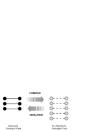
FIG. 6.: This figure illustrate formation of entangled states: a certain number of maximally entangled pairs is manipulated by LOCC and converted into pairs in some state $\rho$. The asymptotic conversion ration is known as the entanglement of formation. The converse of formation is distillation of entanglement. Again, the asymptotic rate of converting pairs in state $\rho$ into maximally entangled states is known as the entanglement of distillations. The two measures of entanglement are in general different, distillation being greater than or equal to formation. This surprising irreversibility of entanglement conversion is explained in the text as a consequence of loss of classical information about the decomposition of $\rho$.

I now introduce the final measure of entanglement which was first proposed in Vedral et al. (1997a). This measure is intimately related to the entanglement of distillation by providing an upper bound for it. If ${\cal D}$ is the set of all disentangled states, the measure of entanglement for a state $\sigma$ is then defined as

Relative entropy of entanglement.

$$E({\sigma}):=\min_{\rho\in{\cal D}}\,\,\,S(\sigma||\rho)$$ (165)

where $S(\sigma||\rho)$ is the quantum relative entropy. This measure, which I will call the relative entropy of entanglement, tells us that the amount of entanglement in $\sigma$ is its distance from the disentangled set of states. In statistical terms introduced in Section II, the more entangled a state is the more it is distinguishable from a disentangled state (Vedral et al., 1997b). To understand better all three measures of entanglement we need to introduce another quantum protocol that relies fundamentally on entanglement.

Another condition which might be considered intuitive for a measure of entanglement is convexity. Namely, we might require that

$$E(\sum_{i}p_{i}\sigma^{i})\leq\sum_{i}p_{i}E(\sigma^{i})$$ (166)

This states that mixing cannot increase entanglement. For example, an equal mixture of two maximally entangled states $|00\rangle+|11\rangle$ and $|00\rangle-|11\rangle$ is a separable state and consequently contains no entanglement. I did not include convexity as a separate requirement for an entanglement measure as it is not completely independent from E3. This is because E3 and the strong additivity ($E(\rho\otimes\sigma)=E(\rho)+E(\sigma)$) imply convexity,

$$n\sum_{i}p_{i}E(\rho_{i}) = E(\rho_{1}^{\otimes p_{1}n}\rho_{2}^{\otimes p_{2}n}...\rho_{N}^{\otimes p_{N}n})$$ (167)

$$\geq E((\sum_{i}p_{i}\rho_{i})^{\otimes n})=nE((\sum_{i}p_{i}\rho_{i}),$$ (168)

where the equalities follow from the strong additivity assumption and the inequality is a consequence of E3. The symbol $\rho^{\otimes m}$ means that we have $m$ copies of the state $\rho$. Nevertheless, it is interesting to point out that any convex measure that satisfies continuity and weak additivity has to be bounded from below by the entanglement of distillation and from above by the entanglement of formation (Horodecki et al., 2000b). We will see that ”most” entanglement measures can in fact be generated using the quantum relative entropy.

It is interesting to note that the relative entropy of entanglement does in fact satisfy both convexity and continuity (Donald and Horodecki, 1999) although not additivity (Vollbrecht and Werner 2000). Furthermore, we can easily show that it is an upper bound to the entanglement of distillation. We have that for any pure state $|\psi\rangle$, $\min_{\omega\in{\cal D}}S(\psi^{\otimes n}||\omega)=min_{\omega\in{\cal D}}-\langle\psi^{\otimes n}|\log\omega|\psi^{\otimes n}\rangle$. But, the logarithmic function is concave so that

$\displaystyle\min_{\omega\in{\cal D}}-\langle\psi^{\otimes n}|\log\omega|\psi^{\otimes n}\rangle\geq\min_{\omega\in{\cal D}}-\log\langle\psi^{\otimes n}|\omega|\psi^{\otimes n}\rangle$

However, according to the recent result of the Horodeckis (Horodecki et al, 1996), since $\omega$ is a disentangled state, then its fidelity with the maximally entangled state cannot be larger than the inverse of the half dimension of that state, so that $\langle\psi^{\otimes n}|\omega|\psi^{\otimes n}\rangle\leq 1/2^{n}.$ Thus,

$$\min_{\omega\in{\cal D}}S(\psi^{\otimes n}||\omega)\geq-\log(1/2^{n})=n$$ (169)

But we know that this minimum is achievable by the state $\omega=\rho^{\otimes n},$ where $\rho$ is obtained from $\psi$ by removing the off-diagonal elements in the Schmidt basis. Consequently, if we are starting with $n$ copies of state $\sigma$, and obtaining $m$ copies of $\psi$ by LOCC, then

$\displaystyle D=\frac{m}{n}=\frac{1}{n}\min_{\omega\in{\cal D}}S(\psi^{\otimes m}||\omega)\leq\frac{1}{n}\min_{\omega\in{\cal D}}S(\sigma^{\otimes n}||\omega)$

where the equality follows from eq.(169) and the inequality from the fact that the relative entropy is non-increasing under LOCC (strictly speaking, $D=\lim_{n\rightarrow\infty}\frac{m}{n}$ and, of course, $m$ is a function of $n$, $m=m(n)$). Thus, the distillable entanglement is bounded from above by the relative entropy of entanglement.

A similar argument can be given to show that the relative entropy of entanglement is bounded from the above by the entanglement of formation (Vedral and Plenio, 1998). Since most of the measures of entanglement can be derived from the relative entropy they will possess this similar property. In order to see this, we first need to introduce quantum teleportation.

B Teleportation

Let us begin by describing quantum teleportation in the form originally proposed by Bennett et al. (1993). Suppose that Alice and Bob, who are distant from each other, wish to implement a teleportation procedure. Initially they need to share a maximally entangled pair of qubits. This means that if Alice and Bob both have one qubit each, then the joint state may for example be:

$$|\Psi_{AB}\rangle=(|0_{A}\rangle|0_{B}\rangle+|1_{A}\rangle|1_{B}\rangle)/\sqrt{2}\;,$$ (170)

where the first ket (with subscript A) belongs to Alice and second (with subscript B) to Bob. Note that this state is maximally entangled and is different from a statistical mixture $(|00\rangle\langle 00|+|11\rangle\langle 11|)/2$ which is the most correlated state allowed by classical physics.

Now suppose that Alice receives a qubit in an unknown state $|\Phi\rangle=a|0\rangle+b|1\rangle$ and she wants to teleport it to Bob. The state has to be unknown to her because otherwise she can just phone Bob up and tell him all the details of the state, and he can then recreate it on a particle that he possesses. Given that Alice does not know the state, she cannot measure it to obtain all the necessary information to specify it. If she could, this would lead to a violation of uncertainty principle. Therefore she has to resort to using the state $|\Psi_{AB}\rangle$ that she shares with Bob to transfer her state to him without actually learning this state. This procedure is what we mean by quantum teleportation.

I first write out the total state of all three qubits

$$|\Phi_{AB}\rangle:=|\Phi\rangle|\Psi_{AB}\rangle=(a|0\rangle+b|1\rangle)(|00\rangle+|11\rangle)/\sqrt{2}\;\;.$$ (171)

However, the above state can be conveniently written in a different basis

$$|\Phi_{AB}\rangle = (a|000\rangle+a|011\rangle+b|100\rangle+b|111\rangle)/\sqrt{2}$$ (172)

$$= \frac{1}{2}[|\Phi^{+}\rangle(a|0\rangle+b|1\rangle)+|\Phi^{-}\rangle(a|0\rangle-b|1\rangle)$$ (173)

$$+ |\Psi^{+}\rangle(a|1\rangle+b|0\rangle)+|\Psi^{-}\rangle(a|1\rangle-b|0\rangle)]\;,$$ (174)

where

$$|\Phi^{+}\rangle = (|00\rangle+|11\rangle)/\sqrt{2}$$ (175)

$$|\Phi^{-}\rangle = (|00\rangle-|11\rangle)/\sqrt{2}$$ (176)

$$|\Psi^{+}\rangle = (|01\rangle+|10\rangle)/\sqrt{2}$$ (177)

$$|\Psi^{-}\rangle = (|01\rangle-|10\rangle)/\sqrt{2}\;$$ (178)

form an ortho-normal basis of Alice’s two qubits (remember that the first two qubits belong to Alice and the last qubit belongs to Bob). The above basis is frequently called the Bell basis. This is a very useful way of writing the state of Alice’s two qubits and Bob’s single qubit because it displays a high degree of correlations between Alice’s and Bob’s parts: for every state of Alice’s two qubits (i.e. $|\Phi^{+}\rangle,|\Phi^{-}\rangle,|\Psi^{+}\rangle,|\Psi^{-}\rangle$) there is a corresponding state of Bob’s qubit. In addition the state of Bob’s qubit in all four cases ”looks very much like” the original qubit that Alice has to teleport to Bob. It is now straightforward to see how to proceed with the teleportation protocol (Bennett et al., 1993):

1. Upon receiving the unknown qubit in state $|\Phi\rangle$ Alice performs projective measurements on her two qubits in the Bell basis. This means that she will obtain one of the four Bell states randomly, and with equal probability.

2. Suppose Alice obtains the state $|\Psi^{+}\rangle$. Then the state of all three qubits (Alice $+$ Bob) collapses to the following state

   $$|\Psi^{+}\rangle(a|1\rangle+b|0\rangle)\;.$$ (179)

   (the last qubit belongs to Bob as usual). Alice now has to communicate the result of her measurement to Bob (over the phone, for example). The point of this communication is to inform Bob how the state of his qubit now differs from the state of the qubit Alice was holding before the Bell measurement.

3. Now Bob has to apply a unitary transformation on his qubit which simulates a logical NOT operation: $|0\rangle\rightarrow|1\rangle$ and $|1\rangle\rightarrow|0\rangle$. He thereby transforms the state of his qubit into the state $a|0\rangle+b|1\rangle$, which is precisely the state that Alice had to teleport to him initially. This completes the protocol. It is easy to see that if Alice obtained some other Bell state, then Bob would have to apply some other simple operation to complete the teleportation. They can be represented by the Pauli spin matrices.

An important fact to observe in the above protocol is that all the operations (Alice’s measurements and Bob’s unitary transformations) are local in nature. This means that there is never any need to perform a (global) transformation or measurement on all three qubits simultaneously, which is what allows us to call the above protocol a genuine teleportation. It is also important that the operations that Bob performs are independent of the state that Alice tries to teleport to him. Note also that the classical communication from Alice to Bob in step 2 above is crucial because otherwise the protocol would be impossible to execute (there is a deeper reason for this: if we could perform teleportation without classical communication then Alice could send messages to Bob faster than the speed of light, see e.g. Vedral et al. (1997c)).

It is important to observe that the fact that the initial state to be teleported is destroyed immediately after Alice’s measurement, i.e it becomes maximally mixed of the form $(|0\rangle\langle 0|+|1\rangle\langle 1|)/2$. This has to happen since otherwise Alice and Bob would end up with two qubits in the same state. So, effectively, they would clone an unknown quantum state, which is impossible by the laws of quantum mechanics. This is the no-cloning theorem of Wootters and Zurek (1982), which is a simple consequence of linearity of quantum dynamical laws. We also see that at the end of the protocol the quantum entanglement of $|\Psi_{AB}\rangle$ is completely destroyed. Does this have to be the case in general or might we save that state at the end (by perhaps performing a different teleportation protocol)? The answer is yes (Plenio and Vedral, 1998), and the reason is that if this was not the case, then entanglement could increase under LOCC, which as we have seen is prohibited by definition.

Teleportation has been experimentally performed in three different set-ups (Bouwmeester et al., 1997). It will now be used to link the three measures of entanglement. I will show that all different measures of entanglement can be understood as special cases of the relative entropy of entanglement (Henderson and Vedral, 2000). This unification relies on adding an ancilla, which I will call a memory system and which will help us keep track of the various decompositions of a given bi-partite density matrix. How much access is available to this memory determines which measure of entanglement is used.

C Measures of entanglement from relative entropy

Suppose that Alice and Bob share a state described by the density matrix $\rho_{AB}$. The state $\rho_{AB}$ has an infinite number of different decompositions $\varepsilon=\{\left|\psi_{AB}^{i}\right\rangle\langle\psi_{AB}^{i}|,p_{i}\}$, into pure states $\left|\psi_{AB}^{i}\right\rangle$, with probabilities $p_{i}$. We denote the mixed state $\rho_{AB}$ written in decomposition $\varepsilon$ by

$$\rho_{AB}^{\varepsilon}=\sum_{i}p_{i}\left|\psi_{AB}^{i}\right\rangle\langle\psi_{AB}^{i}|$$ (180)

As we have seen measures of entanglement are associated with formation and distillation of pure and mixed entangled states. The known relationships between the different measures of entanglement for mixed states are $E_{D}(\rho_{AB})\leq E_{RE}(\rho_{AB})\leq E_{F}(\rho_{AB})$, (Vedral and Plenio, 1998). Equality holds for pure states, where all the measures reduce to the Von Neumann entropy, $S(\rho_{A})=S(\rho_{B})$.

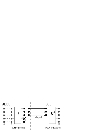
FIG. 7.: This figure illustrates formation of a state by LOCC and with the help of teleportation. First, Alice creates the joint state of subsystems $A$ and $B$ locally. Then, she performs the quantum data compression on the subsystem $B$ and teleports the compressed state to Bob. Finally, Bob decompresses the received state and hence Alice and Bob end up sharing the joint state of $A$ and $B$ initially prepared by Alice.

Formation of an ensemble of $n$ non-maximally entangled pure states, $\rho_{AB}=\left|\psi_{AB}\right\rangle\langle\psi_{AB}|$ is achieved by the following protocol. Alice first prepares the states she would like to share with Bob locally. She then uses Schumacher compression, (Schumacher, 1995), to compress subsystem $B$ into $nS(\rho_{B})$ states. Subsystem $B$ is then teleported to Bob using $nS(\rho_{B})$ maximally entangled pairs. Bob decompresses the states he receives and so ends up sharing $n$ copies of $\rho_{AB}$ with Alice. The entanglement of formation is therefore $E_{F}(\rho_{AB})=S(\rho_{B})$. For pure states, this process requires no classical communication in the asymptotic limit (Lo and Popescu, 1999). The reverse process of distillation is accomplished using the Schmidt projection method (Bennett et al, 1996a), which allows $nS(\rho_{B})$ maximally entangled pairs to be distilled in the limit as $n$ becomes very large. No classical communication between the separated parties is required. Therefore pure states are fully inter-convertible in the asymptotic limit.

The situation for mixed states is more complex. When any mixed state, denoted by Eq.(180), is created, it may be imagined to be part of an extended system whose state is pure. The pure states $|\psi_{AB}^{i}\rangle$ in the mixture may be regarded as correlated to orthogonal states $|m_{i}\rangle$ of a memory $M$. The extended system is in the pure state $\left|\psi_{MAB}\right\rangle=\sum_{i}\sqrt{p_{i}}|m_{i}\rangle|\psi_{AB}^{i}\rangle$. If we have no access to the memory system, we trace over it to obtain the mixed state in Eq.(180). In fact, the lack of access to the memory is of a completely general nature. It may be due to interaction with another inaccessible system, or it may be due to an intrinsic loss of information. The results I will present are universally valid and do not depend on the nature of the information loss. We will see that the amount of entanglement involved in the different entanglement manipulations of mixed states depends on the accessibility of the information in the memory at different stages. Note that a unitary operation on $\left|\psi_{MAB}\right\rangle$ will convert it into another pure state $\left|\phi_{MAB}\right\rangle$ with the same entanglement, and tracing over the memory yields a different decomposition of the mixed state. Reduction of the pure state to the mixed state may be regarded as due to a projection-valued measurement on the memory with operators $\{E_{i}=\left|m_{i}\right\rangle\langle m_{i}|\}$.

Consider first the protocol of formation by means of which Alice and Bob come to share an ensemble of $n$ mixed states $\rho_{AB}$ as in Fig. 7. Alice first creates the mixed states locally by preparing a collection of $n$ states in a particular decomposition, $\varepsilon=\{\left|\psi_{AB}^{i}\right\rangle\langle\psi_{AB}^{i}|,p_{i}\}$ by making $np_{i}$ copies of each pure state $|\psi_{AB}^{i}\rangle$. At the same time we may imagine a memory system entangled to the pure states to be generated, which keeps track of the identity of each member of the ensemble. I consider first the case where the state of subsystems $A$ and $B$ together with the memory is pure. Later, I will consider the situation in which Alice’s memory is decohered. There are then three ways for her to share these states with Bob. First of all, she may simply compress subsystem $B$ to $nS(\rho_{B})$ states, and teleport these to Bob using $nS(\rho_{B})$ maximally entangled pairs. The choice of which subsystem to teleport is made so as to minimise the amount of entanglement required, so that $S(\rho_{B})\leq S(\rho_{A})$. The teleportation in this case would require no classical communication in the asymptotic limit, just as for pure states (Lo and Popescu, 1999). The state of the whole system which is created by this process is an ensemble of pure states $\left|\psi_{MAB}\right\rangle$, where subsystems $M$ and $A$ are on Alice’s side and subsystem $B$ is on Bob’s side. In terms of entanglement resources, however, this process is not the most efficient way for Alice to send the states to Bob. She may do it more efficiently by using the memory system of $\left|\psi_{MAB}\right\rangle$ to identify blocks of $np_{i\text{ }}$members in each pure state $\left|\psi_{AB}^{i}\right\rangle$, and applying compression to each block to give $np_{i}S(\rho_{B}^{i})$ states. Then the total number of maximally entangled pairs required to teleport these states to Bob is $n\sum_{i}p_{i}S(\rho_{B}^{i})$, which is clearly less than $nS(\rho_{B})$, by concavity of the entropy. The amount of entanglement required clearly depends on the decomposition of the mixed state $\rho_{AB}$. In order to decompress these states, Bob must also be able to identify which members of the ensemble are in which state. Therefore Alice must also send him the memory system. She now has two options. She may either teleport the memory to Bob, which would use more entanglement resources. Or she may communicate the information in the memory classically, with no further use of entanglement. When Alice uses the minimum entanglement decomposition, $\varepsilon=\{\left|\psi_{AB}^{i}\right\rangle\langle\psi_{AB}^{i}|,p_{i}\}$, this process, originally introduced by Bennett et al., (1996b), makes the most efficient use of entanglement, consuming only the entanglement of formation of the mixed state, $E_{F}(\rho_{AB})=\sum_{i}p_{i}S(\rho_{B}^{i})$. We may think of the classical communication between Alice and Bob in one of two equivalent ways. Alice may either measure the memory locally to decohere it, and then send the result to Bob classically, or she may send the memory through a completely decohering quantum channel. Since Alice and Bob have no access to the channel, the state of the whole system which is created by this process is the mixed state

$$\rho_{ABM}^{\varepsilon}=\sum_{i}p_{i}|\psi_{AB}^{i}\rangle\langle\psi_{AB}^{i}|\otimes|m_{i}\rangle\langle m_{i}|$$ (181)

where Bob is classically correlated to the $AB$ subsystem. Bob is then able to decompress his states using the memory to identify members of the ensemble.

Once the collection of $n$ pairs is shared between Alice and Bob, it is converted into an ensemble of $n$ mixed states $\rho_{AB}$ by destroying access to the memory which contains the information about the state of any particular member of the ensemble. It is the loss of this information which is responsible for the fact that entanglement of distillation is lower than entanglement of formation, since it is not available to parties carrying out the distillation. If Alice and Bob, who do have access to the memory, were to carry out the distillation, they could obtain as much entanglement from the ensemble as was required to form it. In the case where Alice and Bob share an ensemble of the pure state $\left|\psi_{MAB}\right\rangle$, they would simply apply the Schmidt projection method, (Bennett et al., 1996a). The relative entropy of entanglement gives the upper bound to distillable entanglement, $E_{RE}(\left|\psi_{(MA):B}\right\rangle\langle\psi_{(MA):B}|)=S(\rho_{B})$, which is the same as the amount of entanglement required to create the ensemble of pure states, as described above. Here $MA$ and $B$ are spatially separated subsystems on which joint operations may not be performed. In my notation, I use a colon to separate the local subsystems.

On the other hand, if Alice used the least entanglement for producing an ensemble of the mixed state $\rho_{AB}$, together with classical communication, the state of the whole system is an ensemble of the mixed state $\rho_{ABM}^{\varepsilon}$, and the process is still reversible. Because of the classical correlation to the states $\left|\psi_{AB}^{i}\right\rangle$, Alice and Bob may identify blocks of members in each pure state $\left|\psi_{AB}^{i}\right\rangle$, and apply the Schmidt projection method to them, giving $np_{i}S(\rho_{B}^{i})$ maximally entangled pairs, and hence a total entanglement of distillation of $\sum_{i}p_{i}S(\rho_{B}^{i})$. The relative entropy of entanglement again quantifies the amount of distillable entanglement from the state $\rho_{ABM}^{\varepsilon}$ and is given by $E_{RE}(\rho_{A:(BM)}^{\varepsilon})=\min_{\sigma_{ABM}\in D}S(\rho_{ABM}^{\varepsilon}||\sigma_{ABM})$. The disentangled state which minimises the relative entropy is $\sigma_{ABM}=\sum_{i}p_{i}\sigma_{AB}^{i}\otimes|m_{i}\rangle\langle m_{i}|$, where $\sigma_{AB}^{i}$ is obtained from $|\psi_{AB}^{i}\rangle\langle\psi_{AB}^{i}|$ by deleting the off-diagonal elements in the Schmidt basis. This is the minimum because the state $\rho_{MAB}$ is a mixture of the orthogonal states $\left|m_{i}\right\rangle|\psi_{AB}^{i}\rangle$, and for a pure state $|\psi_{AB}^{i}\rangle$, the disentangled state that minimises the relative entropy is $\sigma_{AB}^{i}$. The minimum relative entropy of the extended system is then

$$S(\rho_{ABM}^{\varepsilon}||\sigma_{ABM})=\sum_{i}p_{i}S(\rho_{B}^{i})$$ (182)

This relative entropy, $E_{RE}(\rho_{A:(BM)}^{\varepsilon})$, has previously been called the ‘entanglement of projection’ (Garisto and Hardy, 1999), because the measurement on the memory projects the pure state of the full system into a particular decomposition. The minimum of $E_{RE}(\rho_{A:(BM)}^{\varepsilon})$ over all decompositions is equal to the entanglement of formation of $\rho_{AB}$. However, Alice and Bob may choose to create the state $\rho_{AB}$ by using a decomposition with higher entanglement than the entanglement of formation. The maximum of $E_{RE}(\rho_{A:(BM)}^{\varepsilon})$ over all possible decompositions is called the ‘entanglement of assistance’ of $\rho_{AB}$ (DiVicenzo et al., 1998). Because $E_{RE}(\rho_{A:(BM)}^{\varepsilon})$ is a relative entropy, it is invariant under local operations and non-increasing under general operations, properties which are conditions for a good measure of entanglement (Vedral and Plenio, 1998). However, unlike $E_{RE}(\rho_{AB})$ and $E_{F}(\rho_{AB})$, it is not zero for completely disentangled states. In this sense, the relative entropy of entanglement, $E_{RE}(\rho_{A:(BM)}^{\varepsilon})$, defines a class of entanglement measures interpolating between the entanglement of formation and entanglement of assistance. Note that an upper bound for the entanglement of assistance, $E_{A}$, can be shown using concavity (DiVicenzo et al., 1998), to be $E_{A}(\rho_{AB})\leq\min[S(\rho_{A}),S(\rho_{B})]$. This bound can also be shown from the fact that the distillable entanglement from any decomposition, $E_{RE}(\rho_{A:(BM)}^{\varepsilon})\leq E_{A}(\rho_{AB})$ cannot be greater than the entanglement of the original pure state.

Note that here we are really creating a state $\rho^{\otimes n}=\rho\otimes\rho\ldots\rho$. The entanglement of formation of such a state is, strictly speaking, given by $E_{F}(\rho^{\otimes n})$; so, the entanglement of formation per one single pair is $E_{F}(\rho^{\otimes n})/n$. It is at present not clear if this is the same as $E_{F}(\rho)$ in general, i.e. whether the entanglement of formation is additive. Bearing this in mind we continue our discussion whose conclusions will not depend on the validity of the additivity assumption of the entanglement of formation (for more on this issues see for example Hayden et al, 2000).

We may also derive relative entropy measures that interpolate between the relative entropy of entanglement and the entanglement of formation (Horodecki et al., 2000b) by considering non-orthogonal measurements on the memory. First of all, the fact that the entanglement of formation is in general greater than the upper bound for entanglement of distillation, emerges as a property of the relative entropy, namely that it cannot increase under the local operation of tracing one subsystem (this is property F2 of the quantum relative entropy given in Section II) (Lindblad 1974),

$$E_{F}(\rho_{AB}) = \min_{\sigma_{ABM}\in{\cal D}}S(\rho_{ABM}||\sigma_{ABM})$$ (183)

$$\geq \min_{\sigma_{AB}\in{\cal D}}S(\rho_{AB}||\sigma_{AB})$$ (184)

In general, the loss of the information in the memory may be regarded as a result of an imperfect classical channel. This is equivalent to Alice making a non-orthogonal measurement on the memory, and sending the result to Bob. In the most general case, $\{E_{i}=A_{i}A_{i}^{+}\}$ is a POVM (positive operator valued measure; loosely speaking, this is a CP map as in eq. (50) where all the individual outcomes are recorded) performed on the memory. The decomposition corresponding to this measurement is composed of mixed states, $\xi=\{q_{i},Tr_{M}(A_{i}\rho_{MAB}A_{i}^{+})\}$, where $q_{i}=Tr(A_{i}\rho_{MAB}A_{i}^{+})$. The relative entropy of entanglement of the state $\rho_{MAB}^{\xi}$, when $\xi$ is a decomposition of $\rho_{AB}$ resulting from a non-orthogonal measurement on $M$, defines a class of entanglement measures interpolating between the relative entropy of entanglement and the entanglement of formation of the state $\rho_{AB}$. In the extreme case where the measurement gives no information about the state $\rho_{AB}$, $E_{RE}(\rho_{A:(BM)}^{\varepsilon})$ becomes the relative entropy of entanglement of the state $\rho_{AB}$ itself. In between, the measurement gives partial information. So far, I have shown that the measures interpolating between entanglement of assistance and entanglement of formation result from making orthogonal measurements on preparations of the pure state $\left|\psi_{MAB}\right\rangle$ in different bases. I note that they may equally be achieved by using the preparation associated with entanglement of assistance, and making increasingly non-orthogonal measurements.

D Classical Information and Quantum correlations

The loss of entanglement may be related to the loss of information in the memory. There are two stages at which distillable entanglement is lost. The first is in the conversion of the pure state $\left|\psi_{MAB}\right\rangle$ into a mixed state $\rho_{ABM}$. This happens because Alice uses a classical channel to communicate the memory to Bob. The second is due to the loss of the memory, $M$, taking the state $\rho_{ABM}$ to $\rho_{AB}$. The amount of information lost may be quantified by the difference in mutual information between the respective states. Mutual information is a measure of correlations between the memory $M$ and the system $AB$, giving the amount of information about $AB$ which may be obtained from a measurement on $M$. The quantum mutual information between $M$ and $AB$ is defined as $I_{Q}(\rho_{M:(AB)})=S(\rho_{M})+S(\rho_{AB})-S(\rho_{MAB})$. The mutual information loss in going from the pure state $\left|\psi_{MAB}\right\rangle$ to the mixed state in Eq. (181) is $\Delta I_{Q}=S(\rho_{AB})$. There is a corresponding reduction in the relative entropy of entanglement, from the entanglement of the original pure state, $E_{RE}(\left|\psi_{(MA):B}\right\rangle\langle\psi_{(MA):B}|)$, to the entanglement of the mixed state $E_{RE}(\rho_{A:(BM)}^{\varepsilon})$ for all decompositions $\varepsilon$ arising as the result of an orthogonal measurement on the memory. It is possible to prove, using the non-increase of relative entropy under local operations, that when the mutual information loss is added to the relative entropy of entanglement of the mixed state $E_{RE}(\rho_{A:(BM)}^{\varepsilon})$, the result is greater than the relative entropy of entanglement of the original pure state, $E_{RE}(\left|\psi_{(MA):B}\right\rangle\langle\psi_{(MA):B}|)$, (Henderson and Vedral, 2000).  The strongest case, which occurs when $E_{RE}(\rho_{A:(BM)}^{\varepsilon})=E_{F}(\rho_{AB})$, is:

$$E_{RE}(\left|\psi_{(MA):B}\right\rangle\langle\psi_{(MA):B}|)\leq E_{F}(\rho_{AB})+S(\rho_{AB})$$ (185)

A similar result may be proved for the second loss, due to loss of the memory, (Henderson and Vedral, 2000). Again the mutual information loss is $\Delta I_{Q}=S(\rho_{AB})$. The relative entropy of entanglement is reduced from $E_{RE}(\rho_{A:(BM)}^{\varepsilon})$, for any decomposition $\varepsilon$ resulting from an orthogonal measurement on the memory, to $E_{RE}(\rho_{AB})$, the relative entropy of entanglement of the state $\rho_{AB}$ with no memory. When the mutual information loss is added to $E_{RE}(\rho_{AB})$, the result is greater than $E_{RE}(\rho_{A:(BM)}^{\varepsilon})$. In this case, the result is strongest for $E_{RE}(\rho_{A:(BM)}^{\varepsilon})=E_{A}(\rho_{AB})$:

$$E_{A}(\rho_{AB})\leq E_{RE}(\rho_{AB})+S(\rho_{AB})$$ (186)

Notice that if $\rho_{AB}$ is a pure state, then $S(\rho_{AB})=0$, and equality holds. Inequalities (185) and (186) provide lower bounds for $E_{F}(\rho_{AB})$ and $\ E_{RE}(\rho_{AB})$ respectively. They are of a form typical of irreversible processes in that restoring the information in $M$ is not sufficient to restore the original correlations between $M$ and $AB$. In particular, they express that the loss of entanglement between Alice and Bob at each stage must be accompanied by an even greater reduction in mutual information between the memory and subsystems $AB$. The general result can be derived from Donald’s equality (Donald, 1986). We have in general that for any $\sigma$ and $\rho=\sum_{i}p_{i}\rho_{i}$ the following is true

$$S(\rho||\sigma)+\sum_{i}p_{i}S(\rho_{i}||\rho)=\sum_{i}p_{i}S(\rho_{i}||\sigma)$$ (187)

Suppose that $E(\rho)=S(\rho||\sigma)$. Then, since $E(\rho_{i})\leq S(\rho_{i}||\sigma)$, we have the following inequality

$$E(\rho)+\sum_{i}p_{i}S(\rho_{i}||\rho)\geq\sum_{i}p_{i}E(\rho_{i})$$ (188)

Thus, the loss of entanglement in $\{p_{i},\rho_{i}\}\rightarrow\rho$ is bounded from above by the Holevo information

$$\sum_{i}p_{i}E(\rho_{i})-E(\rho)\leq\sum_{i}p_{i}S(\rho_{i}||\rho)$$ (189)

This is a physically pleasing property of entanglement. It says that the amount of information lost always exceeds the lost entanglement, which indicates that entanglement stores only a part of information - the rest, of course, is stored in classical correlations. (see also Eisert et al, 2000, who consider a similar problem, although not in the full generality of the above analysis).

In summary, the relative entropy of entanglement of the state $\rho_{AB}$ depends only on the density matrix $\rho_{AB}$, and gives an upper bound to the entanglement of distillation. The other measures of entanglement, which are given by relative entropies of an extended system, all depend on how the information in the memory is used, or how the density matrix is decomposed. There are numerous decompositions of any bipartite mixed state into a set of states $\rho_{i}$ with probability $p_{i}$. The average entanglement of states in each decomposition is given by the relative entropy of entanglement of the system extended by a memory whose orthogonal states are classically correlated to the states of the decomposition. This correlation records which state $\rho_{i}$ any member of an ensemble of mixed states $\rho_{AB}^{\otimes n}$ is in. It is available to parties involved in formation of the mixed state, but is not accessible to parties carrying out distillation. When the classical information is fully available, different decompositions give rise to different amounts of distillable entanglement, the highest being entanglement of assistance and the lowest, entanglement of formation. If access to the classical record is reduced, the amount of distillable entanglement is reduced. In the limit where no information is available, the upper bound to the distillable entanglement is given by the relative entropy of entanglement of the state $\rho_{AB}$ itself, without the extension of the classical memory.

I close this section by discussing generalisations to more than two subsystems. First of all it is not at all clear how to perform this in the case of entanglement of formation and distillation. The former one just does not have a natural generalisation and, for the later one, it is not clear what states should we be distilling when we have three or more parties. The relative entropy of entanglement on the other hand does not suffer from this problem (Vedral and Plenio, 1998; Vedral et al., 1997b). Its definition for N parties would be $E_{RE}(\sigma):=\min_{\rho\in D}S(\sigma||\rho)$ where $\rho=\sum_{i}p_{i}\rho^{i}_{1}\otimes\rho^{i}_{2}...\otimes\rho^{i}_{N}$.

I will now use the knowledge we have gained of classical and quantum correlations to describe quantum computation. It will be seen, perhaps somewhat surprisingly, that classical correlations will play a more prominent role than quantum correlations in the speed-up of certain quantum algorithms.

V Quantum computation

A quantum computer is a physical system that can accept input states which represent a coherent superposition of many different possible basis states and subsequently evolve them into a corresponding superposition of outputs. Computation, i.e. a sequence of unitary transformations, affects simultaneously each element of the superposition, generating a massive parallel data processing albeit within one piece of quantum hardware. In this way quantum computers can efficiently solve some problems that are believed to be intractable on classical computers (Deutsch and Josza, 1992) (the best example is Shor’s factorisation algorithm (Shor, 1996)). Therefore the advantage of a quantum computer lies in the exploitation of the phenomenon of superposition. The great importance of the quantum theory of computation is in the fact that it reveals the fundamental connections between the laws of physics and the nature of computation (Deutsch, 1998).

In order to understand the efficiency of computer algorithms, we have to discuss the theory of computational complexity. I will only mention the basics, but a more detailed account can be found in e.g. (Papadimitriou, 1995). Computational complexity concerns the difficulty of solving certain problems, such as for example multiplication of two numbers, finding the minimum of a given function and so on. Complexity theory divides problems into two basic categories:

1. easy problems: the time of computation $T$ is a polynomial function of the size of the input $l$, i.e. $T=c_{n}l^{n}+...+c_{1}l+c_{0}$, where the coefficients $c$ are determined by the problem.

2. hard problems: the time of computation is an exponential function of the size of the input (e.g. $T=2^{cl}$, where c is problem dependent).

The size of the input is always measured in bits (qubits). For example, if we are to store the number $15$, then we need $4$ bits. In general, to store a number N we need about $l=\log N$, where the base of the logarithm is $2$.

The division of problems into ‘easy’ and ‘hard’ is, of course, very rough. First of all, in computation, apart from time, there are other resources which might matter, such as space, energy and so on. If time grows polynomially, but we require an exponentially increasing energy, then the problem is clearly difficult. Also, suppose that the time complexity of one problem is $10^{10}n$ and of another one is $10^{-10}2^{n}$. Then for small $n$ (say $n=10$), the second algorithm, in spite of being exponential, is clearly more efficient. These two issues exemplify that the division into hard and easy problems is not without its own problems. However, this classification system is very simple to put into practice and does illuminate many different aspects of computational problems which is why it is so widely used. I refer the reader to the book by Garey and Johnson (1979) which presents an introduction to hard problems and their detailed classification.

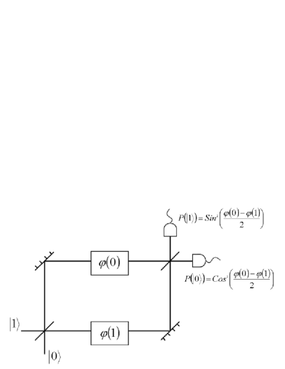
FIG. 8.: The Mach-Zender interferometer. A photon is split at a beam-splitter and can take two different paths. In each of the paths we have a different phase introduced to the photon state, so that, after it encounters the second beam-splitter, the probabilities of detection in two branches have the sinusoidal dependance on the phase difference. In terms of quantum computation, the beam-splitter implements the Hadamard transform and the whole interferometer can be seen as implementing Deutsch’s algorithm (see text for explanation).

There is a great simplification in understanding quantum computation: a quantum computer is formally equivalent to a multiparticle ”Mach-Zender like” interferometer (Cleve et al., 1997). I first present the simplest kind of interferometer in terms of its function as a simple computer. We see from the Fig. 8 that the path of the photon is in fact a quantum bit in the sense that the photon can be in a superposition of the two paths. The first beam splitter acts as the unitary evolution $|0\rangle\rightarrow|0\rangle+|1\rangle$ which is known as the Hadamard gate. Next is the phase shift which has the following effect

$$|0\rangle \rightarrow e^{i\phi(0)}|0\rangle$$ (190)

$$|1\rangle \rightarrow e^{i\phi(1)}|1\rangle$$ (191)

At the end we have another beam splitter and two detector measuring contributions to the state $|0\rangle$ and $|1\rangle$. The corresponding probabilities of detection are

$$P_{0} = \cos^{2}\frac{\phi(0)-\phi(1)}{2}$$ (192)

$$P_{1} = \sin^{2}\frac{\phi(0)-\phi(1)}{2}$$ (193)

If, for example, $\phi(0)=\phi(1)$, then only the detector $0$ will be registering counts. If, on the other hand $\phi(0)=\phi(1)\pm\pi$, then only detector $1$ will be registering counts. These two situations are basically identical to what is known as Deutsch’s algorithm (Deutsch, 1985), the first algorithm to give an indication that quantum computers are more powerful than their classical counterparts. This algorithm has also implemented experimentally in Nuclear Magnetic Resonance (NMR) (Jones and Mosca, 1998a).

A Deutsch’s algorithm

Deutsch’s problem (Deutsch, 1985) is the simplest possible example which illustrates the advantages of quantum computation. The problem is the following. Suppose that we are given a binary function of a binary variable $f:\{0,1\}\longrightarrow\{0,1\}$. Thus, $f(0)$ can either be $0$ or $1$, and $f(1)$ likewise can either be $0$ or $1$, giving altogether four possibilities. However, suppose that we are not interested in the particular values of the function at $0$ and $1$, but we need to know whether the function is: 1) constant, i.e. $f(0)=f(1)$, or 2) varying, i.e. $f(0)\neq f(1)$. Now Deutsch poses the following task: by computing $f$ only once determine whether it is constant or varying. This kind of problem is generally referred to as a promise algorithm, because one property out of a certain number of properties is initially promised to hold, and our task is to determine computationally which one holds (see also (Deutsch and Josza, 1992) for other similar types of promise algorithms).

First of all, classically finding out in one step whether a function is constant or varying is clearly impossible. We need to compute $f(0)$ and then compute $f(1)$ in order to compare them. There is no way out of this double evaluation. Quantum mechanically, however, there is a simple method to achieve this task by computing $f$ only once! Two qubits are needed for the computation. In reality only one qubit is really needed, but the second qubit is there to implement the necessary transformation. We can imagine that the first qubit is the input to the quantum computer whose internal (hardware) part is represented by the second qubit. The computer itself will implement the following transformation on the two qubits (we perform this fully quantum mechanically, i.e. we are now not using ”classical” devices such as beam splitters):

$$|x\rangle|y\rangle\longrightarrow|x\rangle|y\oplus f(x)\rangle\;,$$ (194)

where $x$ is the input qubit and $y$ the hardware, as depicted in Fig. 9. Note that this transformation is reversible and thus there is a unitary transformation to implement it (but we will not pay any attention to that at the moment, as we are only interested here in the basic principle). Note also that $f$ has been used only once. The trick is to prepare the input in such a state that we make use of quantum superpositions. Let us have at the input

$$|x\rangle|y\rangle=(|0\rangle+|1\rangle)(|0\rangle-|1\rangle)\;,$$ (195)

where $|x\rangle$ is the actual input and $|y\rangle$ is part of the computer hardware. Thus before the transformation is implemented, the state of the computer is in an equal superposition of all four basis states, which we obtain by simply expanding the state in eq. (195),

$$|\Psi_{\mbox{in}}\rangle=|00\rangle-|01\rangle+|10\rangle-|11\rangle\;.$$ (196)

Note that there are negative phase factors before the second and fourth term. When this state now undergoes the transformation in eq. (194), we have the following output state

$$|\Psi_{\mbox{out}}\rangle = |0f(0)\rangle-|0\overline{f(0)}\rangle+|1f(1)\rangle-|1\overline{f(1)}\rangle$$ (197)

$$= |0\rangle(|f(0)\rangle-|\overline{f(0)}\rangle)+|1\rangle(|f(1)\rangle-|\overline{f(1)}\rangle)\;,$$ (198)

where the bar indicates the opposite of that value, so that, for example, $\overline{0}=1$. Now we see where the power of quantum computers is fully realised: each of the components in the superposition of $|\Psi_{\mbox{in}}\rangle$ underwent the same evolution of eq. (194) “simultaneously”, leading to the powerful “quantum parallelism” (Deutsch, 1985). This feature is true for quantum computation in general. Let us look at the two possibilities now:

1. if $f$ is constant then

   $$|\Psi_{\mbox{out}}\rangle=(|0\rangle+|1\rangle)(|f(0)\rangle-|\overline{f(0)}\rangle)\;.$$ (199)

2. if $f$ is varying then

   $$|\Psi_{\mbox{out}}\rangle=(|0\rangle-|1\rangle)(|f(0)\rangle-|\overline{f(0)}\rangle)\;.$$ (200)

Note that the output qubit (the first qubit) emerges in two different orthogonal states, depending on the type of $f$. These two states can be distinguished with $100$ percent efficiency. This is easy to see if we first perform a Hadamard transformation on this qubit, leading to the state $|0\rangle$ if the function is constant, and to the state $|1\rangle$ if the function is varying. Now a single projective measurement in $0,1$ basis determines the type of the function. Therefore unlike their classical counterparts quantum computers can solve Deutsch’s problem.

Let us now rephrase this in terms of phase shifts to emphasise its underlying identity with the above Mach-Zender interferometer. The transformation of the two registers is the following

$$|x\rangle|-\rangle\Rightarrow e^{i\pi f(x)}|x\rangle|-\rangle$$ (201)

where $x=0,1$ and $|-\rangle=|0\rangle-|1\rangle$. Thus, the first qubit is like a photon in the interferometer, receiving a conditional phase shift depending on its state ($0$ or $1$). It is left to the reader to show that this transformation is formally identical to the above analysis. The second qubit is there just to implement the phase shift quantum mechanically. It should be emphasised that this quantum computation, although extremely simple, contains all the main features of successful quantum algorithms: it can be shown that all quantum computations are just more complicated variations of Deutsch’s problem (Cleve et al, 1997). We will use the introduction of a phase shift as a basic element of a quantum computer and relate this to the notion of distinguishability and relative entropy.

Note one important aspect: the input could also be of the form $|-\rangle|-\rangle$. A constant function would then lead to the state $|-\rangle|-\rangle$ and a varying function would lead to $|+\rangle|-\rangle$. So, the $|+\rangle$ and $|-\rangle$ are equally good as input states of the first qubit and both lead to quantum speed-up. Their equal mixture, on the other hand, is not. This means that the output would be an equal mixture $|+\rangle\langle+|+|-\rangle\langle-|$ no matter whether $f(0)=f(1)$ or $f(0)\neq f(1)$, i.e. the two possibilities would be indistinguishable. Thus for quantum algorithm to work well, we need the first register to be highly correlated to the two different types of functions. So, if the output state of the first qubit $\rho_{1}$ indicates that we have a constant function and $\rho_{2}$ that we have a varying function, then the efficiency of Deutsch’s algorithm depends on how well we can distinguish the two states $\rho_{1}$ and $\rho_{2}$. This is given by the Holevo bound

$$H=S(\rho)-\frac{1}{2}(S(\rho_{1})+S(\rho_{2}))$$ (202)

where $\rho=1/2(\rho_{1}+\rho_{2})$. Thus if $\rho_{1}=\rho_{2}$, then $H=0$ and the quantum algorithm has no speed up over the classical one. One the other extreme, if $\rho_{1}$ and $\rho_{2}$ are pure and orthogonal, then $H=1$ and the computation gives the right result in one step. In between these two extremes lie all other computations with varying degree of efficiency as quantified by the Holevo bound. Note that these are purely classical correlations and that there is no entanglement between the first and the second qubit. In fact the Holevo bound is the same as the formula I suggested for classical correlations in the previous section. The key to understanding the efficiency of Deutsch’s algorithm is therefore through the mixedness of the first register. If the initial state has the entropy of $S_{0}$, then the final Holevo bound is

$$S(\rho)-S_{0}$$ (203)

So the more mixed the first qubit the less efficient the computation. Note that the quantum mutual information between the first two qubits is zero throughout the entire computation (so there are neither classical nor quantum correlations between them).

B Computation: Communication in time

Can we extend the above entropic analysis to other algorithms as well? The answer is yes and this is exactly what I will describe next (Bose et al, 2000b). To explain why this is so, I first need to introduce a few definitions and a communication model of quantum computation. We have two programmers, the sender and the receiver and two registers, the memory ($M$) register and the computational ($C$) register. The sender prepares the memory register in a certain quantum state $|i\rangle_{M}$ which encodes the problem to be solved. For example, in the case of factorization (Shor, 1996), this register will store the number to be factored. In case of a search (Grover, 1996), this register will store the state of the list to be searched. The number $N$ of possible states $|i\rangle_{M}$ will, of course, be limited by the greatest number that the given computer could factor or the largest list that it could search. The receiver then prepares the computational register in some initial state $\rho^{0}_{C}$. Both the sender and the receiver feed the registers (prepared by them) to the quantum computer. The quantum computer implements the following general transformation on the registers

$$(|i\rangle\langle i|)_{M}\otimes\rho^{0}_{C}\rightarrow(|i\rangle\langle i|)_{M}\otimes U_{i}\rho_{C}^{0}U_{i}^{\dagger}.$$ (204)

The resulting state $\rho_{C}(i)=U_{i}\rho^{0}_{C}U_{i}^{\dagger}$ of the computational register contains the answer to the computation and is measured by the receiver. As the quantum computation should work for any $|i\rangle_{M}$, it should also work for any mixture $\sum_{i}^{N}p_{i}(|i\rangle\langle i|)_{M}$, where $p_{i}$ are probabilities. For the sender to use the above computation as a communication protocol, he has to prepare any one of the states $|i\rangle_{M}$ with an apriori probability $p_{i}$. The entire input ensemble is thus $\sum_{i}^{N}p_{i}(|i\rangle\langle i|)_{M}\otimes\rho^{0}_{C}$. Due to the quantum computation, this becomes

$$\sum_{i}^{N}p_{i}(|i\rangle\langle i|)_{M}\otimes\rho^{0}_{C}\rightarrow\sum_{i}^{N}p_{i}(|i\rangle\langle i|)_{M}\otimes\rho_{C}(i).$$ (205)

Whereas before the quantum computation, the two registers where completely uncorrelated (mutual information is zero), at the end, the mutual information becomes

$$I_{MC}: = S(\rho_{M})+S(\rho_{C})-S(\rho_{MC})$$ (206)

$$= S(\rho_{C})-\sum_{i}^{N}p_{i}S(\rho_{C}(i)),$$ (207)

where $\rho_{M}$ and $\rho_{C}$ are the reduced density operators for the two registers, $\rho_{MC}$ is the density operator of entire $M+C$ system and $S(\rho)=-\mbox{Tr}\rho\log\rho$ is the von Neumann entropy (for conventional reasons we will use $\log_{2}$ in all calculations). Notice that the value of the mutual information (i.e correlations) is equal to the Holevo bound $H=S(\rho_{C})-\sum_{i}^{N}p_{i}S(\rho_{C}(i))$ for the classical capacity of a quantum communication channel (Holevo, 1973) (Note that $\rho_{C}=\sum_{i}^{N}p_{i}\rho_{C}(i)$). This tells us how much information the receiver can obtain about the choice $|i\rangle_{M}$ made by the sender by measuring the computational register. The maximum value of $H$ is obtained when the states $\rho_{C}(i)$ are pure and orthogonal. Moreover, the sender conveys the maximum information when all the message states have equal apriori probability (which also maximizes the channel capacity). In that case the mutual information (channel capacity) at the end of the computation is $\log{N}$. Thus the communication capacity $I_{MC}$ (given by Eq.(206)) gives an index of the efficiency of a quantum computation. A necessary target of a quantum computation is to achieve the maximum possible communication capacity consistent with given initial states of the quantum computer. We cannot give a sufficiency criterion from our general approach as this depends on the specifics of an algorithm. If one breaks down the general unitary transformation $U_{i}$ of a quantum algorithm into a number of successive unitary blocks, then the maximum capacity may be achieved only after number of applications of the block. In each of the smaller unitary blocks, the mutual information between the $M$ and the $C$ registers (i.e the communication capacity) increases by a certain amount. When its total value reaches the maximum possible value consistent with a given initial state of the quantum computer, the computation is regarded as being complete.

C Black box complexity

Any general quantum algorithm has to have a certain number of queries into the memory register (Bennett et al., 1997; Beals et al, 1998; Ambainis, 2000) (this is necessitated by the fact that the transformation on the computational register has to depend on the problem at hand, encoded in $|i\rangle_{M}$). These queries can be considered to be implemented by a black box into which the states of both the memory and the computational registers are fed. The number of such queries needed in a certain quantum algorithm gives the black box complexity of that algorithm (Bennett et al., 1997; Beals et al., 1998; Ambainis, 2000) and is a lower bound on the complexity of the whole algorithm. The black box approach is a simplification for looking at the complexity of an algorithm. A black box allows us to perform a certain computation without having its exact details. It is possible that physical implementations of a particular black box may prove to be difficult. So when we estimate the complexity of an algorithm by counting the number of applications of a black box, we have to bear in mind that there might an additional complexity component arising in physical implementation.

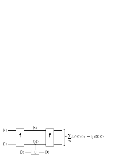
FIG. 9.: This figure represents a network that implements the phase flip operation given the black box computing the function $f(x)$. The unitary transformation $U$ implements $|0\rangle\rightarrow-|0\rangle$ conditionally on the value of $f(x)$.

In general we have a function $f:\{0,1\}^{n}\rightarrow\{0,1\}$ (so the function maps $n$-bit values to either $0$ or $1$). Quantum algorithms, such as database search, can be expressed in this form (in the case of database search, all the values of $f$ are $0$ apart from one which is equal to $1$; the task is to find this value). The black box is assumed to be able to perform the transformation $|x\rangle|y\rangle\rightarrow|x\rangle|f(x)\oplus y\rangle$, just like in Deutsch’s algorithm. We have the freedom to represent this black box transformation as a phase flip which is equivalent in power (up to a constant factor as seen in Fig. 9),

$$|x\rangle|y\rangle\rightarrow(-1)^{f(x)\oplus y}|x\rangle|y\rangle$$ (208)

Recently, Ambainis (2000) showed in a very elegant paper that if the memory register was prepared initially in the superposition $\sum_{i}^{N}|i\rangle_{M}$, then, in a search algorithm, $O(\sqrt{N})$ queries would be needed to completely entangle it with the computational register. This gives a lower bound on the number of queries in a search algorithm. In a manner analogous to his, we will calculate the change in mutual information between the memory and the computational registers (from Eq.(206)) in one query step. The number of queries needed to increase the mutual information to $\log{N}$ (for perfect communication between the sender and the receiver), is then a lower bound on the complexity of the algorithm.

D Database search

Any search algorithm (whether quantum or classical, irrespective of its explicit form), will have to find a match for the state $|i\rangle_{M}$ of the $M$ register among the states $|j\rangle_{C}$ of the $C$ register and associate a marker to the state that matches (Here, $|j\rangle_{C}$ is a complete orthonormal basis for the $C$ register). The most general way of doing such a query in the quantum case is the black box unitary transformation (Ambainis, 2000)

$$U_{B}|i\rangle_{M}|j\rangle_{C}=(-1)^{\delta_{ij}}|i\rangle_{M}|j\rangle_{C}.$$ (209)

Any other unitary transformation performing a query matching the states of the $M$ and the $C$ registers, could be constructed from the above type of query. Note that the black box is able to recognize if a value in the $C$ register is the same as the solution, but is unable to explicitly provide that solution for us. For example, imagine that Socrates goes to visit the all-knowing Ancient Greek oracle (black box) who is only able to answer with ”yes” or ”no”. Suppose further that Socrates wants to know who the wisest person in the world is. He would then have to ask something like ”Is Plato the wisest person in the world?” and would not be able to ask directly ”Who is the wisest person in the world?”. This ”yes-no” approach is typical for any black box analysis. The advantage of using this black box quantum mechanically is that we can query all the individual elements of the superposition simultaneously. Although we can identify the solution in one step quantum mechanically, further computations are required to amplify the right solution so that the subsequent measurement is more likely to reveal it.

I would like to put a bound on the change of the mutual information in one such black box step. Let the memory states $|i\rangle_{M}$ be available to the sender with equal apriori probability so that the communication capacity is a maximum. His initial ensemble is then $\frac{1}{N}\sum_{i}^{N}(|i\rangle\langle i|)_{M}$. Let the receiver prepare the $C$ register in an initial pure state $\psi^{0}$ (in fact, the power of quantum computation stems from the ability of the receiver to prepare pure state superpositions of form $\frac{1}{N}\sum_{j}^{N}|j\rangle_{C}$). This is an equal weight superposition of all $|j\rangle_{C}$ as there is no apriori information about the right $|j\rangle_{C}$. This can be done by performing a Hadamard transformation to each qubit of the $C$ register. In general, there will be many black box steps on the initial ensemble before a perfect correlation is set up between the $M$ and the $C$ registers. Let, after the $k$th black box step, the state of the system be

$$\rho^{k}=\frac{1}{N}\sum_{i}^{N}(|i\rangle\langle i|)_{M}\otimes(|\psi^{k}(i)\rangle\langle\psi^{k}(i)|)_{C}$$ (210)

where

$$|\psi^{k}(i)\rangle_{C}=\sum_{j}\alpha_{ij}^{k}|j\rangle_{C}.$$ (211)

The $(k+1)$th black box step changes this state to $\rho^{k+1}=\frac{1}{N}\sum_{i}^{N}(|i\rangle\langle i|)_{M}\otimes(|\psi^{k+1}(i)\rangle\langle\psi^{k+1}(i)|)_{C}$ with

$$|\psi^{(k+1)}(i)\rangle=\sum_{i,j}^{N}\alpha_{ij}^{k}(-1)^{\delta_{ij}}|j\rangle_{C}.$$ (212)

Thus we only have to evaluate the difference of mutual information between the $M$ and the $C$ register for the states. This difference of mutual information (when computed from Eq.(206)) can be shown to be the difference $|S(\rho^{k+1}_{C})-S(\rho^{k}_{C})|$ (Henderson and Vedral, 2000). This quantity is bounded from the above by (Fannes, 1999)

$$|S(\rho^{k+1}_{C}) - S(\rho^{k}_{C})|\leq d_{B}(\rho^{k}_{C},\rho^{k+1}_{C})\log{N}$$ (213)

$$- d_{B}(\rho^{k}_{C},\rho^{k+1}_{C})\log{d_{B}(\rho^{k}_{C},\rho^{k+1}_{C})}$$ (214)

where, $d_{B}(\sigma,\rho)=\sqrt{1-F^{2}(\sigma,\rho)}$ is the Bures metric (Bures, 1969) and $F(\sigma,\rho)=\mbox{Tr}\sqrt{\sqrt{\rho}\sigma\sqrt{\rho}}$ is the fidelity. Using methods similar to Ambainis (2000), it can be shown that $F(\rho^{0}_{C},\rho^{1}_{C})\geq\frac{N-2}{N}$ from which it follows that the change in the first step

$$|S(\rho^{0}_{C})-S(\rho^{1}_{C})|\leq\frac{3}{\sqrt{N}}\log{N}.$$ (215)

The change $|S(\rho^{k}_{C})-S(\rho^{k+1}_{C})|$ in the subsequent steps has to be less than or equal to the change in the first step. This is because the Bures metric does not increase under general completely positive maps (which is what the query represents when we trace out the $M$ register). Any other operations performed only on the $C$ register in between two queries can only reduce the mutual information between the $C$ and the $M$ register. This means that at least $O(\sqrt{N})$ steps are needed to produce full correlations (maximum mutual information of value $\log{N}$) between the two registers. This gives the black box lower bound on the complexity of any quantum search algorithm. Of course, we know that there also exists an algorithm achieving this bound due to Grover (1996) and this has been proven to be optimal (Bennett et al., 1996a; Ambainis, 2000; Zalka, 1999). However, the proof presented here is the most general as it holds even when any type of completely positive map is allowed between the queries (only in Zalka (1999) a heuristic argument was made for the optimality of Grover’s algorithm under general operations). Grover’s algorithm has also been implemented experimentally (Jones and Mosca, 1998b).

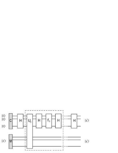
FIG. 10.: The figure shows the circuit for Grover’s algorithm. $C$ is the computational register and $M$ is the memory register. $U_{B}$ is the black box query transformation, $H$ is a Hadamard transformation on every qubit of the $C$ register and $f_{0}$ is a phase flip in front of the $|00...0\rangle_{C}$. The block consisting of $H,U_{B},H$ and $f_{0}$ is repeated a number of times.

I now use Grover’s algorithm to show how the mutual information varies with time in a quantum search. The general sequence described by Cleve et. al (1997) for Grover’s algorithm will be used in this letter. The algorithm consists of repeated blocks, each consisting of a Hadamard transform on each qubit of the $C$ register, followed by a $U_{B}$ (our black box transformation), followed by another Hadamard transform on each qubit of the $C$ register and finally a phase flip $f_{0}$ of the $|00...0\rangle_{C}$ state of the $C$ register (See Fig. 10). This block can then be repeated as many times as is necessary to bring the mutual information to its maximum value of $\log{N}$, which, as I have shown in Eq.(215) to be $O(\sqrt{N})$. Note that the only transformation correlating the $M$ and $C$ registers is the black box transformation $U_{B}$ and all the other transformations are done only on the $C$ register and therefore do not change the mutual information between the two registers. In Fig. 8 I have plotted the variation of mutual information between the $M$ and the $C$ registers (i.e the communication capacity of the quantum computation) with the number of iterations of the block in Grover’s algorithm. It is seen that the mutual information oscillates with the number of iterations. Fig. 11 is plotted for a four qubit computational register which can search a database of $16$ entries. It is seen that the period is roughly $6$, which means that the number of steps needed to achieve maximum mutual information is roughly $3$. This is well above our bound for the minimum number of steps, which is $4/3$ in this case.

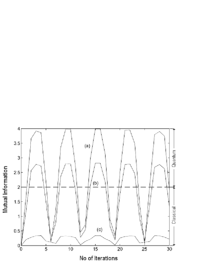
FIG. 11.: The figure shows the dependence of the mutual information between the $M$ and the $C$ registers as a function of the number of times the block in Grover’s algorithm is iterated for various values of initial mixedness of the $C$ register. Each qubit of the $C$ register is initially in the state $p|0\rangle\langle 0|+(1-p)|1\rangle\langle 1|$, (a) $p=1$, (b) $p=0.95$ and (c) $p=0.7$. The (a) and (b) computations achieve higher mutual information than classically allowed in the order of root $N$ steps, while (c) does not.

The fact that the mutual information oscillates periodically (or more precisely, ”quasi”-periodically) follows from the quantum Poincare recurrence theorem (Hogg and Huberman, 1983). Namely, if the system has a discrete spectrum and is ”driven” by a periodic potential (as is in Grover’s case, where we repeat the same operation time and again), then its wavefunction $\psi(t)$ will undergo a quasi periodic motion, i.e. for any $\epsilon>0$, there exists a relatively dense set $\{T_{\epsilon}\}$ such that

$$||\psi(t+T_{\epsilon})-\psi(t)||<\epsilon$$ (216)

for all time $t$ and for each $T_{\epsilon}$ in the set. This is exactly the behavior seem in the Fig. 9. The distance between the two states $|\psi\rangle=\sum_{i}a_{i}|i\rangle$ and $|\phi\rangle=\sum_{j}b_{j}|j\rangle$ is defined in the usual way

$$||\psi-\phi||:=\sum_{i}|a_{i}-b_{i}|$$ (217)

The three graphs (a), (b) and (c) in Fig. 9 are for different values of initial mixedness of the $C$ register. We find that the mutual information fails to rise to the maximum value of $\log{N}$ when the state of the computational register is mixed. Our formalism thus allows us to calculate the performance of a quantum computation as a function of the mixedness (quantified by the von Neumann entropy) of the computational register. We can put a bound on the entropy of the second register after which the quantum search becomes as inefficient as the classical search. If the initial entropy $S(\rho^{0}_{C})$ of the $C$ register exceeds $\frac{1}{2}\log{N}$, then the change in mutual information between the $M$ and the $C$ registers in the course of the entire quantum computation would be at most $\log{\sqrt{N}}$. This can be achieved by a classical database search in $\sqrt{N}$ steps. So there is no advantage in using quantum evolution when the initial state is too mixed. Note that our condition

Sufficient condition for no quantum speed-up.

$$S(\rho^{0}_{C})\geq\frac{1}{2}\log{N}$$ (218)

Note that this is only a sufficient and not a necessary condition.

I also point out that the states of the $M$ register need not be a mixture, but could be an arbitrary superposition of states $|i\rangle_{M}$ (such a state was used by Ambainis in his argument (Ambainis, 2000)). All the above arguments still hold in that case, and the $M$ and the $C$ registers become quantum mechanically entangled and not just classically correlated. Thus our analysis implies that any quantum computation is mathematically identical to a measurement process (Everett, 1973). The system being measured is the $M$ register and the apparatus is the $C$ register of the quantum computer. As the time progresses the apparatus (register $C$) becomes more and more correlated (or entangled) to the system (register $M$). This means that the states of register $C$ become more and more distinguishable which allows us to extract more information about the $M$ register by measuring the $C$ register. The analysis in the last paragraph, where I showed the limitations on the efficiency of quantum computation imposed by the mixedness of the $C$ register, applies also to the efficiency of a quantum measurement when the apparatus is in a mixed state. Mixedness of an apparatus, to the best of our knowledge, has never been considered in the analysis of quantum measurement. In general practice, any apparatus, however macroscopic, is considered to be in a pure quantum state before the measurement. Our approach highlighting the formal analogy between measurement and computation offers a way to analyse measurement in a much more general context.

Finally, I would like to discuss what would happen if we decided to change the nature of the Black box. Suppose that instead of being able to recognize the right solution, the black box is much more powerful and it can compare if the individual bit values coincide with the bit values of the solution. So, for all $k$,

$$|i_{0}i_{1}...i_{k}...i_{n}\rangle|j_{0}i_{j}...j_{k}...j_{n}\rangle\rightarrow$$ (219)

$$(-1)^{\delta_{i_{k}j_{k}}}|i_{0}i_{1}...i_{k}...i_{n}\rangle|j_{0}i_{j}...j_{k}...j_{n}\rangle,$$ (220)

where $i=i_{0}i_{1}...i_{k}...i_{n}$ and $j=j_{0}i_{j}...j_{k}...j_{n}$ are the binary representations of $i$ and $j$ respectively. Then, it can easily be checked that this gate has the power to correlate the $C$ and the $M$ register by the amount of $\log 2$. Therefore the search algorithm would take $\log N$ steps (instead of $\sqrt{N}$), i.e. it would be polynomial instead of exponential! There is, of course, a hidden complexity here which is in constructing the new Black box from the original Black Box. It can be shown that this requires exponential increase in time (or space which can always be traded for time) and this then compensates the exponential decrease in the number of applications of the new Black Box. In fact, this new black box is equivalent to the Ancient Greek oracle being able to answer to Socrates ”Who is the wisest person in the world?”.

Can we use entropic measures of the above form to quantify complexity of other quantum algorithms? The answer is unclear at present. The only algorithm that presently achieves an exponential speed-up over its classical counterpart, Shor’s factorisation algorithm (Shor, 1996), cannot be usefully re-phrased in terms of black box operations (more precisely, it is rather trivial, as it requires only one black box operation!). However, this does not prevent us from deriving fundamental bounds on information storage and the speed of its processing based on the Uncertainty principle. In the next subsection, I show the ultimate limits of processing power no matter what model of computation is used so long as it uses quantum systems (particles or fields alike).

Quantum computation and quantum measurement. I now show that quantum computation is formally identical to a quantum measurement as described by von Neumann (1955). The analysis will be performed in the most general continuous case. Suppose that we have a system $S$ (described by a continuous variable $x$) and an apparatus $A$ (described by a continuous variable $y$ interacting via a Hamiltonian $H=xp$, where $p$ is the momentum of $A$ (we will assume that $\hbar=1$). Suppose in addition that the initial state of the total system is

$$|\Psi(0)\rangle=\int_{x}\phi(x)|x\rangle dx\otimes\eta(y)|y\rangle dy$$ (221)

in an uncorrelated state. The action of the above Hamiltonian then transforms the state into an entangled state. In order to calculate this transformation it will be beneficial to introduce the (continuous) Fourier transform

$$\mbox{F}_{y}:|y\rangle\rightarrow\int e^{-iyp}|p\rangle dp$$ (222)

which takes us from the position space of $A$ into the momentum space of $A$. This is important because we know the effect of the Hamiltonian in the momentum basis. Now, the action of the unitary transformation generated by $H$ is

$$|\Psi(t)\rangle = e^{-ixpt}|\Psi(0)\rangle$$ (223)

$$= \mbox{F}_{y}e^{-ixpt}\mbox{F}_{y}|\Psi(0)\rangle$$ (224)

$$= \int_{x}\int_{y}\phi(x)\eta(y-xy)|x\rangle|y\rangle dxdy$$ (225)

and we see that $S$ and $A$ are now correlated in $x$ and $y$. This means that by measuring $A$ we can obtain some information about the state of $S$. The mutual information $I_{AS}=H(x)+H(y)-H(x,y)$ can be shown to satisfy (Everett, 1973)

$$I_{AS}\geq\ln t$$ (226)

i.e. it is growing at a rate faster than logarithm of time passage during the measurement. This gives us a lower bound to exactly how quickly correlations can be established between the system and the apparatus. This is analogous to the way I derived the upper bound on the efficiency of quantum search algorithms in Section V.

I now show the detailed calculation of the effect of measurement Hamiltonian. Let us define

$$\xi(p):=\mbox{F}_{y}\{\eta(y)\}$$ (227)

The evolution then proceeds as follows,

$$|\Psi(t)\rangle = e^{-xpt}\int_{x}\phi(x)|x\rangle dx\otimes\eta(y)|y\rangle dy$$ (228)

$$= e^{-xpt}\int_{x}\phi(x)\int_{p}\{\int_{y}\eta(y)e^{-iyp}dy\}|x\rangle|p\rangle dxdp$$ (229)

$$= e^{-xpt}\int_{x}\int_{p}\ \phi(x)\xi(p)|x\rangle|p\rangle dxdp$$ (230)

$$= \int_{x}\ \phi(x)\int_{y}\{\int_{p}\xi(p)e^{-ixpt}e^{iyp}dp\}|x\rangle|y\rangle dxdy$$ (231)

$$= \int_{x}\int_{y}\phi(x)\eta(y-xy)|x\rangle|y\rangle dxdy$$ (232)

This result has the same formal structure of quantum algorithms presented before: a Fourier transform, followed by a conditional phase shift and then followed by another Fourier transform (c.f. Deutsch’s and Grover’s algorithms). Therefore we can see that how efficiently we can measure something is the same as how efficiently we can compute, both of which depend on how quickly we can establish correlations.

E Ultimate limits of computation: The Bekenstein bound

Given a computer enclosed in a sphere of radius $R$ and having available the total amount of energy $E$ what is the amount of information that it can store and how quickly can this information be processed? The Holevo bound gives us the ultimate answer. The amount of information that can be written into this volume is bounded from the above by the entropy, i.e. the number of distinguishable states that this volume can support. I will now use a simple, informal argument to obtain this ultimate bound (Tipler, 1994), but the rigorous derivation can be found in (Bekenstein, 1981). The bound on energy implies a bound on momentum and the total number of states in the phase space is

$$N=\frac{PR}{\Delta P\Delta R}\leq\frac{PR}{\hbar}$$ (233)

where the inequality follows from the Heisenberg uncertainty relations $\Delta P\Delta R\geq\hbar$ which limits the size of the smallest volume in the phase space to $\hbar$ in each of the three spatial directions. From relativity we have that for any particle $p\leq E/c$, so that

$$I\leq\ln N\leq N\leq\frac{E}{c}\frac{R}{\hbar}\leq\frac{ER}{\hbar c}$$ (234)

which is known as the Bekenstein bound. In reality this inequality will most likely be a huge over-estimate, but it is important to know that no matter how we encode information we cannot perform better than is given by our most accurate present theory - quantum mechanics. As an example consider a nucleus of the Hydrogen - according to the above result it can encode about $100$ bits of information (I assumed that $E=mc^{2}$ and that $R=10^{-15}$m). At present, NMR quantum computation achieves ”only” one bit per nucleus (and not per nucleon!)- spin ”up” and spin ”down” are the two states.

From the Bekenstein bound we can derive a bound on the efficiency of information processing. Again my derivation will be loose, and a much more careful calculation confirms what I will present (Bekenstein, 1984). All the bits in the volume $V$ cannot be processed faster than it takes light to travel across $V=4/3\pi R^{3}$, which is $2R/c$. This gives

$$\frac{dI}{dt}\leq\frac{E}{2\hbar}$$ (235)

Again a Hydrogen nucleus can process $10^{24}$ bits per second, which is also in sharp contrast with NMR quantum computation where a NOT gate takes roughly a few milliseconds leading to a maximum of $10^{3}$ bits per second.

The Bekenstein bound shows that there is a potentially great number of under-used degrees of freedom in any physical system. This provides hope that quantum computation will be an experimentally realisable goal. At present, there is a number of different practical implementations of quantum computation, but none of them can store and manipulate more than $10$ qubits at a time ($5$ was the largest number (Vandersypen, 2000) manipulated in a genuine quantum computation process when this review was finished in the summer of $2000$). The above calculation, however, does not take into account the environmental influence on computation nor the experimental precision. I have not at all touched on the practical possibility of building a quantum computer. This is partly for reasons of space, partly because it would spoil the flow of exposition and partly because there is already a number of excellent reviews of this subject (Steane, 1997). It is generally acknowledged that the difficulties in building a quantum computer are only of practical nature and there are no fundamental limits that prohibit such a device. I hope that this section offers convincing arguments that building a quantum computer is a very much worthwhile adventure, both from the technological as well as fundamental perspective. In any case we see that there is a great deal of currently unused potential in physical systems in which to store and encode information. As our level of technology improves we will find more and more ways of getting closed to the Bekenstein bound.

VI Conclusions

We have seen how distinguishability of different physical states is at the heart of information processing, which we quantified using the relative entropy. The relative entropy told us about the possibility of confusing two probability distributions, or, in the quantum case, two density matrices. We have seen that relative entropy never increases under any general quantum evolution, meaning that states can become only less distinguishable as time progresses. The most important consequence of this was shown to be the Holevo bound, which is the bound on the capacity for classical communication using quantum states. This basically told us that $n$ qubits cannot store more than $n$ classical bits of information. While this appears to be a severe limitation on quantum information processing, I showed with the aid of dense coding that quantum communication is in some sense more efficient than its classical counterpart. Dense coding involved the use of entangled states and I therefore showed how the quantum relative entropy can be used to quantify entanglement. Moreover, I used the Holevo bound to put limits on the efficiency of quantum computation by treating it as a communication protocol. Quantum algorithms were shown to be considerably more efficient for some problems than classical algorithms. In particular, I have shown in a new way that the quantum database search has a square root speed up over the classical database search. Efficiency of quantum computation stems from the trade-off between two opposite effects: on the one hand, superpositions allow us to compute in parallel, while, on the other hand, the Holevo bound limits the amount of information we can extract from a quantum state. I also emphasised links between the black box quantum computation and quantum measurement and I showed that there is a fundamental limit to deleting information, leading to Landauer’s principle that $1$ bit erased increases the environment information by $k_{B}\ln 2$.

With every new physical theory comes a new understanding of the world we live in. Through Newtonian physics we understood the Universe as a clockwork mechanism. With the subsequent development of thermodynamics the Universe became a big Carnot engine, slowly evolving towards its final equilibrium state after which no useful work could be obtained - the heat death. Presently, we see Universe as an information processing machine - a computer. Limits to the amount of information it can contain and process are given by the most accurate theory we have, quantum mechanics, giving rise to quantum information theory.

If there is a single moral to be drawn from the relationship between information and physics it is that, as we dig deeper into the fundamental laws on physics, we also push back the boundaries of information processing. It will not be surprising if all the results presented in this review are superseded by higher level generalisation of which they become an approximation in the same way that today classical information theory approximates quantum information theory.

Acknowledgments. I would like to thank S. Bose, D. Deutsch, D. P. Divincenzo, M. J. Donald, A. Ekert, L. Henderson, P. Hayden, J. A. Jones, E. Kashefi, P. L. Knight, G. Lindblad, M. Murao, M. Ozawa, M. B. Plenio, L. Rallan, B. Schumacher and G. Vidal for many stimulating discussions on the subject of quantum information. In particular, I thank L. Rallan for very thorough reading of this manuscript and helping me draw some of the figures. Work for this review has been supported by the Knight Trust and ORS Award, Elsag-Bailey spa, Hewlett-Packard company, EPSRC and the European Union project EQUIP (contract IST-1999-11053).

REFERENCES

- [1] Ambainis, A., 2000, Quantum lower bounds by quantum arguments, quant-ph/0002066.
- [2] Araki, H., and E. H. Lieb, 1970, Comm. Math. Phys., 18, 160.
- [3] Barnum, H., M. A. Neilsen and B. Schumacher, (1998), Phys. Rev. A 57, 4153.
- [4] Beals, R., H. Buhrman, R. Cleve, M. Mosca and R. de Wolf, 1998, Quantum lower bounds by polynomials, Proceedings of FOCS’98, pages 352-361. Also quant-ph/9802049.
- [5] Bekenstein, J. D. , 1981, Physical Review D 23, 287.
- [6] Bekenstein, J. D. , 1984, Physical Review D 30, 1669.
- [7] Bell, J., 1987, ”Speakable and Unspeakable in Quantum Mechanics”, (Cambridge Univ. Press, Cambridge).
- [8] Bennett, C. H., and S. Wiesner, 1992, Phys. Rev. Lett. 69 2881.
- [9] Bennett, C. H., G. Brassard, C. Crepeau, R. Jozsa, A. Peres, and W.K. Wootters, 1993, Phys. Rev. Lett. 70, 1895.
- [10] Bennett, C. H., H. J. Bernstein, S. Popescu, and B. Schumacher, 1996a, Phys. Rev. A 53, 2046.
- [11] Bennett, C. H., D. P. DiVincenzo, J. A. Smolin, and W. K. Wootters, 1996b, Phys. Rev. A 54, 3824.
- [12] Bennett, C. H., E. Bernstein, G. Brassard and U. Vazirani, 1997, SIAM Journal on Computing, 26, 1510. Also quant-ph/9701001.
- [13] Bennett, C. H., D. P. Divincenzo, C. A. Fuchs, T. Mor, E. Rains, P. W. Shor, J. A. Smolin and W. K. Wootters, 1999a, Phys. Rev. A. 59 1070.
- [14] Bennett, C. H., D. P. DiVincenzo, T. Mor, P. W. Shor, J. A. Smolin and B. M. Terhal, 1999b, Phys. Rev. Lett. 82 5385.
- [15] Bhatia, R., 1997, “Matrix Analysis”, (Springer-Verlag, Berlin).
- [16] Bose, S., M. B. Plenio and V. Vedral, 2000a, J. Mod. Opt 47, 291.
- [17] Bose, S., L. Rallan and V. Vedral, 2000b, Phys. Rev. Lett. 85 (25) 5448.
- [18] Bouwmeester, D., J.W. Pan, K. Mattle, M. Eibl, H. Weinfurter, and A. Zeilinger, 1997, Nature 390, 575; D. Boschi, S. Branca, F. DeMartini, L. Hardy, and S. Popescu, Phys. Rev. Lett. 80, 1121 (1998); A. Furusawa et al., Science 282, 706 (1998).
- [19] Bowen, G., 2001, Phys. Rev. A 63 022302.
- [20] Brillouin, L., 1956, “Science and Information Theory”, (Academic Press, New York).
- [21] Bures, D., 1969, Trans. Am. Math. Soc. 135, 199; see also A. Uhlmann, Rep. Math. Phys. 9, 273 (1976); ibid 24, 229 (1986).
- [22] Caves; C. M., and P. D. Drummond, 1994, Rev. Mod. Phys. 66, 481.
- [23] Choi, M. D., 1975, Lin. Algebra and Appl. 10, 285.
- [24] Clauser, J. F., M. A. Horne, A. Shimony, and R. A. Holt, 1969, Phys. Rev. Lett. A 23, 880.
- [25] Cleve, R., A. Ekert, C. Macchiavello and M. Mosca, 1997, Phil. Trans. R. Soc. Lond. A.
- [26] Cover, T. M., and J.A. Thomas, 1991, “Elements of Information Theory” (A Wiley-Interscience Publication).
- [27] Csiszár, I., and J. Körner, 1981, “Coding Theorems for Discrete Memoryless Systems”, (Academic Press, New York).
- [28] Davies, E. B., 1976, ”Quantum Theory of Open Systems”, (Academic Press, London).
- [29] Deutsch, D., 1985, Proc. R. Soc. Lond. A 400, 97; D. Deutsch, Proc. R. Soc. Lond. A 425, 73 (1989).
- [30] Deutsch, D., and R. Jozsa, 1992, Proc. R. Soc. Lond. A 439, 553; E. Bernstein and U. Vazirani, in Proc. 25th ACM Symposium on the Theory of Computation, 11 (1993); D.S. Simon, Proceedings of the 35th Annual Symposium on the Foundations of Computer Science, edited by S. Goldwasser (IEEE Computer Society Press, Los Alamitos, CA), 16 (1994).
- [31] Deutsch, D., 1998, “The Fabric of Reality”, (Viking–Penguin Publishers, London).
- [32] DiVincenzo, D. P., 1998 et al., quant-ph/9803033.
- [33] DiVincenzo, D.P., P.W. Shor, J. A. Smolin, B. M. Terhal and A. V. Thapliyal, 2000, Phys. Rev. A 61 062312.
- [34] Donald, M. J., 1986, Comm. Math. Phys. 105, 13; M.J. Donald, Math. Proc. Camb. Phil. Soc., 101, 363 (1987).
- [35] Donald, M. J., 1992, Found. Phys.,22, 1111.
- [36] Donald, M. J., and M. Horodecki, 1999, Physics Letters A 264, 257.
- [37] Einstein, A., B. Podolsky and N. Rosen, 1935, Phys. Rev. 47, 777.
- [38] Eisert, J., T. Felbinger, P. Papadopoulos, M. B. Plenio, and M. Wilkens, 2000, Phys. Rev. Lett. 84 1611.
- [39] Everett, H., III, 1973, “The Theory of The Universal Wavefunction ”, in “The Many–Worlds Interpretation of Quantum Mechanics” edited by B. DeWitt and N. Graham (Princeton University Press).
- [40] Fannes, M., 1973, Commun. Math. Phys. 31, 291; M. Nielsen, Continuity bounds for entanglement, quant-ph/9908086 (1999).
- [41] Feynman, R.P., 1996, “Feynmann Lectures on Computation”, edited by A. J. G. Hey and R. W. Allen, (Addison-Wesley Publishing Company, Inc.).
- [42] Fuchs, C. A., 1996, “Distinguishability and Accessible Information in Quantum Theory”, PhD thesis, The University of New Mexico, Albuquerque, NM (lanl e-print server: quant-ph/9601020).
- [43] Garey, M., and D. Johnson, 1979, “Computers and intractability: a guide to the theory of NP-completeness, (Freeman, San Francisco, 1979).
- [44] Garisto, R., and L. Hardy, 1999, Phys. Rev. A 60, 827.
- [45] Gisin, N., 1996, Phys. Lett. A 210, 151, and references therein.
- [46] Gordon, J. P., 1964, “Noise at Optical Frequences; Information Theory, Quantum Electronics and Coherent Light, Proc. Int. School Phys. “Enrico Fermi, Course XXXI, ed. P. A. Miles, p.p. 156 (Academic Press, New York).
- [47] Grover, L., 1996, A fast quantum mechanical algorithm for database search, Proceedings of the 28th ACM Symposium on Theory of Computing, p. 212. Also quant-ph/9605043.
- [48] Hausladen, P., R. Jozsa, B. Schumacher, M. Westmoreland and W. K. Wootters, 1996, Phys. Rev. A 54, 1869.
- [49] Hayashi, M., 1997, “Asymptotic Attainment for Quantum Relative Entropy”, lanl e-print server: quant-ph/9704040.
- [50] Hayden, P. M. , Horodecki, M. Terhal, B. M., 2000, “The asymptotic entanglement cost of preparing a quantum state”, lanl e-print server no. 0008134.
- [51] Henderson, L., and V. Vedral, 2000, Phys. Rev. Lett. 84, 2263.
- [52] Hiai, F., and D. Petz, 1991, Comm. Math. Phys. 143, 99;
- [53] Hogg, T., and B. A. Huberman, 1983, Phys. Rev. A 28, 22.
- [54] Holevo, A. S., 1973, Problemy Peredachi Informatsii, 9, 3 (1973) [A. S. Kholevo, Problems of Information Transmission, 9, 177]; for the continuous case see H. P. Yuen and M. Ozawa, Phys. Rev. Lett. 70, 363 (1993).
- [55] Holevo, A. S., 1982, “Probabilistic and Statistical Aspects of Quantum Theory”, (North-Holland Publishing Company, Amsterdam).
- [56] Holevo, A. S., 1998, IEEE. T. Inform. Theory 44 269.
- [57] Horodecki, M., P. Horodecki, and R. Horodecki, 1996, Phys. Lett. A 223, 1.
- [58] Horodecki, M., P. Horodecki and R. Horodecki, 1998a, Phys. Rev. Lett. 80 5239.
- [59] Horodecki, M., 1998b, Phys. Rev. A 57 3364.
- [60] Horodecki, M., P. Horodecki and R. Horodecki, 2000a, lanl gov e-print no quant-ph/0006071.
- [61] Horodecki, M., P. Horodecki, R. Horodecki, 2000b, Phys. Rev. Lett. 84, 2014.
- [62] Ingarden, R. S., A. Kossakowski and M. Ohya, 1997, “Information Dynamics and Open Systems - Classical and Quantum Approach”, (Kluwer Academic Publishers, Dordrecht).
- [63] Ingarden, R. S., 1976, Rep. Math. Phys. 10, 43.
- [64] Jaynes, E. T., and F. W. Cummings, 1963, Proc. IEEE 51, 89.
- [65] Jones, J. A. and M. Mosca, 1998a, J. Chem. Phys. 109 1648.
- [66] Jones, J. A., M. Mosca and R. H. Hansen, 1998b, Nature 393 344. I. L. Chuang, N. Gershenfeld, and M. Kubinec, Phys. Rev. Lett. 80, 3408.
- [67] Kolmogorov, A. N., 1950, “Foundations of The Probability Theory”, (Chelsea pub. company, New York).
- [68] Kraus, B., J. I. Cirac, S. Karnas and M. Lewenstein, 2000, Phys. Rev. A 61 062302.
- [69] Kraus, K., 1983, “States, Effects and Operations: Fundamental Notions of Quantum Theory”, Lecture Notes in Physics 180 (Springer, Berlin, 1983); M. Ozawa, J. Math. Phys. 25, 79 (1984).
- [70] Kullback, S., and R.A. Leibler, 1951, Ann. Math. Stat. 22, 79.
- [71] Landauer, R., 1961, IBM J. Res. Dev. 5, 183; C.H. Bennett, IBM J. Res. Dev. 32, 16 (1988); T. Toffoli, Math. Systems Theory 14, 13 (1981).
- [72] Lebedev, D. S., and L. B. Levitin, 1963, Sov. Phys. Dokl. 8 377.
- [73] Lewenstein, M., D. Bruss, J. I. Cirac, B. Kraus, M. Kus, J. Samsonowicz, A. Sanpera and R. Tarrach, 2000, Separability and Distillability in composite quantum systems - a primer, lanl gov e-print server no. 0006064 and references therein.
- [74] Lindblad, G., 1974, Comm. Math. Phys. 39, 111.
- [75] Lindblad, G., 1975, Comm. Math. Phys. 40, 147.
- [76] Lo, H., and S. Popescu, 1999, Phys. Rev. Lett. 83, 1459.
- [77] Mackey, G. W., 1963, “Mathematical Foundations of Quantum Mechanics”, (New York, W. A. Benjamin Inc.).
- [78] von Neumann, J., 1955, “Mathematische Grundlagen der Quantenmechanic” (Springer, Berlin, 1932; English Translation, Princeton University Press, Princeton).
- [79] Ohya, M., and D. Petz, 1993, “Quantum Entropy and Its Use”, Texts and Monographs in Physics, (Berlin: Springer-Verlag).
- [80] Papadimitriou, C. H., 1995, “Computational complexity”, (Addison-Wesley publishing company, New York).
- [81] Partovi, M. H., 1989, Phys. Lett. A 137, 445, and the references therein.
- [82] Penrose, O., 1973, “Foundations of Statistical Mechanics”, (Oxford University Press, Oxford).
- [83] Peres, A., 1996, Phys. Rev. Lett. 77, 1413.
- [84] Peres, A., 1993,“Quantum Theory: Concepts and Methods”, (Kluwer Academic Publishers).
- [85] Plenio, M. B., and V. Vedral, 1998, Cont. Phys. 38, 431.
- [86] Popescu, S., and D. Rohrlich, 1997, Phys. Rev. A 56, R3319.
- [87] Rains, E. M., 1999, Phys. Rev. A 60 173 ; E. M. Rains, 1999, Phys. Rev. A 60 179.
- [88] Redhead, M., 1987, “Incompleteness, Nonlocality and Realism”, (Clarendon Press, Oxford).
- [89] Reed, M., and B. Simon, 1980, “Methods of Modern Mathematical Physics–Functional Analysis”, (Academic Press, New York).
- [90] Sanov, I. N., 1957, Mat. Sbornik (Moscow) 42, 11.
- [91] Schmidt, E., 1907, The original reference is E. Schmidt, “Zur Theorie der linearen und nicht linearen Integralgleichungen”, Math. Annalen 63, 433 (1907), in the context of quantum theory see H. Everett III, in The Many-World Interpretation of Quantum Mechanics, ed. B.S. DeWitt and N. Graham (Princeton University Press, Princeton, 1973) p. 3, and H. Everett III, Rev. Mod. Phys. 29 454 (1957). A graduate level textbook by A. Peres, “Quantum Theory: Concepts and Methods”, (Kluwer, Dordrecht, 1993), Chapt. 5 includes a brief description of the Schmidt decomposition.
- [92] Schrödinger, E., 1935, Naturwissenschaften 23, 807, 823, 844.
- [93] Schumacher, B., 1995, Phys. Rev. A 51, 2738; R. Jozsa and B. Schumacher, J. Mod. Opt. 41, 2343 (1994).
- [94] Schumacher, B., 1996, Phys. Rev. A 54 2614.
- [95] Schumacher, B., and M. D. Westmoreland, 1997, Phys. Rev. A, 56, 131;
- [96] Schumacher, B. W., and M. D. Westmoreland, 2000, Relative entropy in quantum information theory, lanl e-print no. quant-ph/0004045.
- [97] Shannon, C. E., and W. Weaver, 1949, “The Mathematical Theory of Communication”, (University of Illinois Press, Urbana, IL).
- [98] Shor, P. W., 1996, In Proc. Annual Symposium on Foundations of Computer Science, ed. S. Goldwasser. (IEEE Computer Society Press, Nov. 1994) pp. 124-134; for a review of this algorithm see A. Ekert and R. Jozsa, 1996, Rev. Mod. Phys. 68, 733.
- [99] Steane, A., 1997, Appl. Phys. B. 64, 623; D. G. Cory, R. Laflamme, E. Knill, L. Viola, T. F. Havel, N. Boulant, G. Boutis, E. Fortunato, S. Lloyd, R. Martinez, C. Negrevergne, M. Pravia, Y. Sharf, G. Teklemariam, Y. S. Weinstein, W. H. Zurek, ”NMR Based Quantum Information Processing: Achievements and Prospects”, Fortschritte der Physik special issue (2000).
- [100] Stern, T. E., 1960, IEEE Trans. Info. Theory 6, 435.
- [101] Tipler, F. J., 1994, “The Physics of Immortality”, (Bantam Doubleday Dell Publishing Group, Inc., New York).
- [102] Tolman, R. C., 1938, “The Principles of Statistical Mechanics”, (Oxford University Press, Oxford).
- [103] Umegaki, H., 1962, Kodai Math. Sem. Rep. 14, 59.
- [104] Vandersypen, L. M. K., et al., 2000, Experimental realization of order-finding with a quantum computer, lanl e-print no. quant-ph/0007017.
- [105] Vedral, V., M. B. Plenio, M. A. Rippin, and P. L. Knight, 1997a, Phys. Rev. Lett. 78, 2275.
- [106] Vedral, V., M. B. Plenio, K. Jacobs, and P. L. Knight, 1997b, Phys. Rev. A 56, 4452.
- [107] Vedral, V., M. A. Rippin and M. B. Plenio, 1997c, J. Mod. Opt. 44, 2185.
- [108] Vedral, V., and M. B. Plenio, 1998, Phys. Rev. A, 57, 1619.
- [109] Vedral, V., 2000, Proc. Roy. Soc. Lond. A 456, 969.
- [110] Vidal, G., 2000, J. Mod. Opt. 47 355.
- [111] Vollbrecht, K. G. H., and R. F. Werner, 2000, ”Entanglement Measures under Symmetry”, lanl e-print no. quant-ph/0010095.
- [112] Wehrl, A., 1978, Rev. Mod. Phys. 50, 221.
- [113] Werner, R. F., 1989, Phys. Rev. A 40, 4277.
- [114] Wootters, W.K., and W.H. Zurek, 1982, Nature 299, 802.
- [115] Wootters, W. K., 1998, Phys. Rev. Lett 80, 2245.
- [116] Yamamoto, Y., and H. A. Haus, 1986, Rev. Mod. Phys. 58.
- [117] Zalka, C., 1999, Phys. Rev. A 60, 2746.