Two-particle correlations via quasi-deterministic analyzer model

Abstract

We introduce a quasi-deterministic eigenstate transition model of analyzers in which the final eigenstate is selected by initial conditions. We combine this analyzer model with causal spin coupling to calculate both proton-proton and photon-photon correlations, one particle pair at a time. The calculated correlations exceed the Bell limits and show excellent agreement with the measured correlations of [M. Lamehi-Rachti and W. Mittig, Phys. Rev. D 14 (10), 2543 (1976)] and [ A. Aspect, P. Grangier and G. Rogers, Phys. Rev. Lett. 49 91 (1982)] respectively. We discuss why this model exceeds the Bell type limits.

Past efforts to explain two-particle correlation measurements with hidden variable theories combined with probability methods have failed [1, 2, 3]. Could we successfully explain measured correlations by replacing the probability feature by a deterministic decision process, accumulating the distributions one particle pair at a time? A deterministic trajectory model[4] has been previously used to explain ”ghost diffraction” patterns [5]. In a separate more extensive paper [6], we use a quasi-deterministic analyzer model, to explain the law of Malus for in-sequence photon counting. Here, we use this model in detailed calculations to explain the proton-proton correlations of [7], as well as the four-angle photon-photon correlations of Aspect et al. [8, 9].

Polarized beam splitters as well as Stern-Gerlach type analyzers for spinors are eigenvalue splitters. The quasi-deterministic model outlined here is based on eigenvalue selection. To describe this theory we first rewrite certain relations contained in the generic two-component eigenvalue equation in terms of a convenient Stokes variable representation. Stokes representations for both spinors and vectors are similar and well developed [10].

Consider a Hermitian matrix with elements $h_{11}=a$, $h_{22}=d$, $h_{12}=h\exp(-\imath\phi)$, and $h_{21}=h\exp(\imath\phi)$, where $a$, $d$, $h$, and $\phi$ are real. With $\Psi^{T}={\left[\Psi_{x},\Psi_{y}\right]}$, $\Psi_{x}=A_{x}\cos(\beta)\exp(\imath\alpha_{x})$ and $\Psi_{y}=A_{y}\sin(\beta)\exp(\imath(\alpha_{x}+\delta)$, we can extract from the eigenvalue equation $h\Psi=\lambda\Psi$ the following relations [6].

$$\textbf{{P}}\cdot\textbf{{S}}=\pm P_{0}S_{0}$$ (1)

$$S_{3}P_{2}-S_{2}P_{3}=0$$ (2)

$$S_{1}P_{1}=\pm(P_{1})^{2}S_{0}/P_{0}$$ (3)

Here, $S$ and $P$ are Stokes sets that represent the field and matrix respectively and the two signs are associated with the two eigenvalues. The components of $S$ have the standard form $S_{0}=\Psi^{\dagger}\Psi$, $S_{1}=S_{0}\cos(2\beta)$, $S_{2}=S_{0}\sin(2\beta)\cos(\delta)$, and $S_{3}=S_{0}\sin(2\beta)\sin(\delta)$. The components of $P$ are given by $P_{0}=\sqrt{(a-d)^{2}+4h^{2}}$, $P_{1}=P_{0}\cos(2\alpha)$, $P_{2}=P_{0}\sin(2\alpha)\cos(\phi)$ and $P_{3}=P_{0}\sin(2\alpha)\sin(\phi)$, where $\tan(2\alpha)=2h/(a-d)$ and the eigenvalues are given by $\lambda_{\pm}=(a+d\pm P_{0})/2$. Equation (2) means $\sin(\delta-\phi)=0$.

The vectors S and P represent points on the Poincare’ polarization sphere. If an incident field is to make a transition to an eigenstate, equations (1), (2), and (3) must be satisfied. From (3) we see that the eigenstate condition is related to the sign of the product $S_{1}P_{1}$. The Stokes variables rotate with twice the rotation angle of the field components.

The traditional e and o rays of classical macroscopic electro-optics correspond to two points on opposite sides of the Poincare’ sphere indicated by $P_{1}=1$ and $S_{1}=\pm 1$ for one crystal type. The two eigenvalues, on which the separation decision is made, determine the $P$ sphere radius via $\lambda_{+}-\lambda_{-}=P_{0}$, but not the direction of P. For a fixed relative phase $\phi$, this gives one free variable for the matrix Stokes vector.

The point of view here is that the classical matrix Stokes vector used for a macroscopic field of many photons does not necessarily represent the matrix Stokes vector experienced by individual photons. The first assumption of this model (The distributive assumption) is that the P vectors experienced by individual incident pulses are distributed in the one free variable, at least for the surface transition region. For a given incident pulse, we randomly select this degree of freedom of P from a distribution described below.

The second assumption of this model (The deterministic assumption) is that the incident pulse makes a transition to one eigen-channel or the other, and that the choice is made with a deterministic criteria based on initial conditions of the incident pulse at the analyzer and the randomly selected P. From (2) we see that the sign of $S_{1}P_{1}$ indicates the eigen-channel choice. We indicate this product as a function of $z$, the depth into the crystal, as follows.

$$T(z)=S_{1}(z)P_{1}(z)$$ (4)

The deterministic criteria on which the calculations here are based is that the sign of $T(z)$ after the transition is the same as, and determined by the sign of $T(0)$. For a given value for $S_{1}(0)$ and $P_{1}(0)$ we make the eigen-channel decision by testing the sign of $T(0)$. Are the residual deviations of $P_{1}(z)$ from the macroscopic field value only surface affects, rapidly decreasing with depth into the crystal, or, do they extend throughout the crystal? Both cases give the same correlations, and as shown in [6], both cases give rise to the law of Malus. To correctly describe the correlations, or the law of Malus, it is only necessary that the surface value $P_{1}(0)$ is selected from a distribution. Because of averaging, it would be unreasonable to expect to answer this distribution question with experiments using a macroscopic field of many photons.

For a frame attached to the crystal analyzer (say aligned with the e and o rays), we can partition the matrix Poincare’ sphere with hemispheres indicated by the sign of $P_{1}$. However, viewed from a frame attached to one analyzer, this partition for the other analyzer is rotated. With respect to an analyzers attached frame, we choose P by choosing $2\alpha$ via $2\alpha=arg$ where $arg=\arccos(u)-\pi/2$ and $u$ is selected uniformly from the interval $[-1,1]$. For our linear polarizer, we have $\cos(\phi)=\pm 1$ in the crystal frame. Viewed from a frame fixed to the first analyzer, the $\textbf{{P}}^{\prime}$ hemisphere axis for the second analyzer is rotated from the first by $q=\theta$ for spinors and $q=2\theta$ for vectors. In this fixed reference frame, sampling for the second analyzer is made using $2\alpha^{\prime}=arg(u^{\prime})\pm q$ where $u^{\prime}$ is selected uniformly from the interval $[-1,1]$, but independent of $u$. The independence of the selection of $u$ and $u^{\prime}$ represents a local stochastic element of this theory, and is the reason why we call this a quasi-deterministic model.

Pair counts for the four different coincidence combinations are represented here by $N_{++}$ ,$N_{+-}$ , $N_{-+}$ and $N_{--}$ . For instance $N_{+-}$ is the count for the number of pairs with a $(+)$ for the first analyzer an $(-)$ for the second analyzer. The four pair-counts are accumulated, one pair at a time. The correlations are calculated using the function $\gamma(\theta)=(N_{++}+N_{--}-N_{+-}-N_{-+})/N$ [11], where $N=N_{++}+N_{--}+N_{+-}+N_{-+}$ is the total number of pairs counted.

The proton-proton correlations in [7] were measured using two protons in coincidence produced via scattering a proton beam by a hydrogen target. Only a small percent (We assume $3\%$ for the calculations reported here.) of these proton pairs are in the triplet state. Information about the spin correlations of the protons was obtained in [7] via scattering from a carbon target rather than using a Stern-Gerlach apparatus in each beam. The two protons each are incident upon carbon targets. Four detectors are used, two after each carbon target. On one side, the two detectors are positioned in the reaction plane. On the other, the two detectors are rotated out of the reaction plane by an angle $\theta$. This is an azmuthal rotation around the incident beam direction on that side.

For our reference side, we choose a $(1-2-3)$ right handed coordinate system with $P_{3}$ in the beam direction, and $P_{2}$ perpendicular to the plane of the two detectors. With this, one detector is in the $P_{1}\geq 0$ hemisphere and the second detector is in the other. With a similar choice for the other analyzer, its $P_{1}^{\prime}\geq 0$ hemisphere seen in the fixed reference frame is rotated by $\theta$ around the beam axis. This comparison is made after a rotation to account for the non-alignment of the proton beams. For convenience, we use unit normalization and $S_{1}(0)=\cos(2\beta)$ for the spinor incident on the first analyzer side, where $2\beta$ is sampled uniformly from the interval $[0,2\pi)$ . For the triplet case, we set $S_{1}^{\prime}(0)=S_{1}(0)$, and for the singlet case, we set $S_{1}^{\prime}(0)=-S_{1}(0)$. This represents the causal coupling between the two sides.

Calculations are made using about $10000$ pairs at each relative angular setting. For each member of a pair of proton spinor states, the deterministic decision at the analyzer is made via testing the sign of $T(0)$ at each analyzer. For this, recall that $T^{\prime}(0)$ , given in (4), has two factors each of which can have either sign for the rotated analyzer.

Results of calculations assuming that $100\%$ of the proton pairs are mutually orthogonal are shown by the solid circles in Fig. 1. The solid line corresponds to the formula $-\cos(\theta)$ of quantum mechanics for the same case. The deterministic correlations calculated with $3\%$ of the incident pairs parallel and $97\%$ orthogonal are shown by the solid squares in Fig. 1. This curve falls well within the error bars of the measurements of [7]. The proton-proton correlations calculated with this deterministic analyzer model agree well with results of quantum mechanics and with the experimental data [7].

Here we present calculations for four-angle photon-photon correlation [8, 9] in which the two analyzers are set at angles $(a,a^{\prime})$ and $(b,b^{\prime})$. These angles are chosen to give a relative angle of $\theta$ for two of the combinations, $-\theta$ for another combination, and $3\theta$ for the fourth. Each of the four angular settings represents an independent measurement. Here, the correlation function $\gamma(\theta)$ for each case is calculated as described above and the four-angle correlation function is then calculated by $\gamma_{4}(\theta)=2\gamma(\theta)+\gamma(-\theta)-\gamma(3\theta)$. For the input light, we use an isotropic distribution around the beam axis, sampling $2\beta$ uniformly from $[0,2\pi]$. We use $S_{1}^{\prime}(0)=S_{1}(0)$ for the causal coupling.

In Fig. 2 the solid circles indicate the calculated four-angle correlation, and the solid line represents the function $3\cos(2\theta)-\cos(6\theta)$ of quantum mechanics. The two dash lines represent the well known (CHSH) limits [12]. We emphasize that all contributions to each $\gamma(\theta)$ were calculated using the four pair counts only so there is no chance that an accidental scale factor can be included. The calculated results presented in Fig. 2 clearly confirm that the four-angle photon-photon correlations can be explained using this causal quasi-deterministic analyzer model.

In contrasting the above results with previous studies and views on this topic, many questions are raised. In discussions with many colleagues, the questions seem to focus into three. First, if we replaced the deterministic decision at each analyzer with one based on probability, would we get the same results? The answer is no! In studies leading to this work, the author has tried many different hidden variable probability models, and not found one, no matter what sampling distribution used, that agrees with the deterministic model and quantum mechanics. This finding seems to be consistent with the many studies of probability models by previous authors [2, 13].

We have the second question. Since this theory is based on individual photons making transitions to one or the other eigenvalue channel, is it consistent with the Law of Malus? To the author’s mind, this question is more important than asking if this theory can explain photon-photon correlations. We recall that for distributions accumulated from individual photon counting, the law of Malus is postulated as a fundamental starting point. The analysis of this question is the central theme of a separate and more extensive study by the author [6] . The answer is that this theory is not only consistent with the law of Malus, but as shown in [6], it gives rise to it for in-sequence photon counting. We must take double serious any theory that explains both the observed photon-photon correlations and the law of Malus.

A third question is asked. Why do these calculations not respect the Bell limits, in particular the CHSH limits [12] for the four-angle correlation ? First, given the assumptions used, these limits follow rigorously [12]. The answer is that this deterministic model does not respect some assumptions on which this Bell type theorem is based. To elucidate this, consider the analyzer functions $T(0)=S_{1}(0)P_{1}(0)=\cos(2\beta)\cos(arg(u))$ and $T^{\prime}(0)=S_{1}(0)P_{1}^{\prime}(0)=\cos(2\beta)\cos(arg(u^{\prime})\pm 2\theta)$. The independent parameters $u$ and $u^{\prime}$ represents local stochastic features of this theory. Within the distribution range, and depending on the angle $2\theta$ , there are certain values of $u^{\prime}$ for which the second factor in $T^{\prime}(0)$ can be positive, and certain values for which this factor is negative. Because of the stochastic variable $u$ , we cannot know the path of the individual quantum pulse until after we have measured it. However, we still have distribution information. The number of times the second factor in $T^{\prime}(0)$ is positive depends on the angle $2\theta$. The causal link for individual photon pairs is contained in the first two factors of $T(0)$ and $T^{\prime}(0)$. As a consequence, we have correlations in the distributions which depend on the relative angle. The presence of the local stochastic variable, a necessary part of this theory, does not destroy all causal correlation information in the distributions.

Using $\gamma=\sum{A_{i}B_{i}}/N$, with ${A_{i}=\pm 1}$ and ${B_{i}=\pm 1}$, where $A_{i}$ and $B_{i}$ represent the signs of $T(0)$ and $T^{\prime}(0)$ respectively, we can easily arrive at the following inequality.

$$\left|\gamma_{4}\right|\leq\sum{\left|B_{i}(a-b)+B^{\prime}_{i}(a-b^{\prime})\right|}/N$$ (5)

$$+\sum{\left|B_{i}(a^{\prime}-b)-B^{\prime}_{i}(a^{\prime}-b^{\prime})\right|}/N$$ (6)

Because of the angular dependence of the second factor in $T^{\prime}(0)$, the selection of $B_{i}$ depends on the relative angle. If we did not have this relative angular dependence, this inequality would reduce to $\left|\gamma_{4}\right|\leq 2$ of [12]. This angle dependence does not mean that what happens at one analyzer influences what happens at the other. Rather, the angle dependence is created by the causal coupling relative to the analyzer settings.

In this model calculations, we make no use of entangled states. Our calculated results depend on the causal coupling, the deterministic decision at the analyzer and the stochastic matrix model. If we leave one of these out, such as replacing the deterministic process at the analyzer with probability, we can not describe the data. This is a simple theory which can explain the law of Malus for in-sequence photon counting as well as explain some well known two-particle correlations.

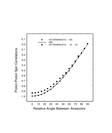
FIG. 1.: Proton-Proton Spin Correlations: Solid circles (Solid squares) indicated deterministic correlations calculated assuming $100\%$ ( $97\%$ ) orthogonal states; Solid line indicates the $-\cos(\theta)$ formula of quantum mechanics.

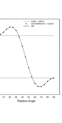
FIG. 2.: Four-Angle Photon-Photon Polarization Correlations: Solid circles indicated deterministic correlations calculated one photon pair at a time; Solid line indicates the $3\cos(2\theta)-\cos(6\theta)$ formula of quantum mechanics.

REFERENCES

- [1] A. Afriat and F. Selleri, The Einstein Podolski and Rosen Paradox, (Plenum Press, New York, 1999).
- [2] F. J. Belinfante, A Survey of Hidden Variable Theories, (Pergamon Press, New York 1973).
- [3] L. E. Ballentine, Am. J. Phys. 55 (9) 785 (1987). 4. D. V.
- [4] B. J. Dalton, in Causality and Locality in Modern Physics, Eds. G. Hunter, S. Jeffers, and J-P. Vigier, (Kluwer-Academic Publishers, Dordrecht, The Netherlands, 1997).
- [5] Strekalov, A. V. Sergienko, D. N. Klyshko, and Y. H. Shih, Phys. Rev. Lett, 74 (18) 3600 (1993).
- [6] Bill Dalton, Law of Malus and Photon-Photon Correlations: A Quasi-Deterministic Analyzer Model, Submitted for publication.
- [7] M. Lamehi-Rachti and W. Mittig, Phys. rev. D 14 (10), 2543 (1976).
- [8] A.Aspect, P. Grangier and G. Rogers, Phys. Rev. Lett. 47 460 (1981).
- [9] A. Aspect, P. Grangier and G. Rogers, Phys. Rev. Lett. 49 91 (1982).
- [10] W. H. McMaster, Am. J. Phys. 22 (6) 351 (1954).
- [11] A. Garuccio and V. Rapisarda, Nuovo Cimento, 65A, 269 (1981).
- [12] J. F. Clauser, M. A. Horne, A. Shimony, and R. A. Holt, Phys. Rev. Lett. 23, 880 (1969).
- [13] D. M.Greenberg, M. A. Horne, A. Shimony and A. Zeilinger, Am. J. Phys. 58, (12) 1131 (1990).