Proposal to test quantum mechanics against macroscopic realism using continuous variable entanglement: a definitive signature of a Schrödinger cat

Abstract

In the Schrödinger-cat gedanken experiment a cat is in a quantum superposition of two macroscopically distinct states, alive and dead. The paradoxical interpretation of quantum mechanics is that the cat is not in one state or the other, alive or dead, immediately prior to its measurement. Because of this apparent defiance of macroscopic reality, quantum superpositions of states macroscopically distinct have generated much interest. Here we address the issue of proving a contradiction with macroscopic reality objectively, through the testable predictions of quantum mechanics. We consider the premises of macroscopic reality (that the “cat” is either “dead” or “alive”, the measurement indicating which) and macroscopic locality (that simultaneous measurements some distance away cannot induce the macroscopic change, “dead” to “alive” and vice versa, to the “cat”). The predictions of quantum mechanics for certain states, generated using states exhibiting continuous variable entanglement, are shown to be incompatible with the predictions of all theories based on this dual premise. Our proof is along the lines of Bell’s theorem, but where all relevant measurements give macroscopically distinct results.

Schrödinger${}^{\cite[cite]{[\@@bibref{Number}{1}{}{}]}}$ raised the issue of the existence and interpretation of the quantum superposition of two macroscopically distinct states in his famous Schrodinger-cat gedanken experiment. A particle is in a quantum superposition of having escaped the nucleus, or otherwise. The presence of the particle outside the nucleus will trigger a lethal device that will kill a cat located in a box. An observer later looks into the box to determine the state of the cat, whether dead or alive. The application of quantum mechanics, to all stages of the sequence of interactions, would ultimately predict the cat to be in a superposition of a state $|1\rangle$, where the cat is dead, and a state $|-1\rangle$, where the cat is alive.

It is a basic feature of quantum mechanics that the quantum superposition state $(|+\rangle+|-\rangle)/\sqrt{2}$ cannot be regarded as classical mixture, where the system is considered to be in state $|+\rangle$ with probability $1/2$, or in state $|-\rangle$ with probability $1/2$. Yet to say in this case that the cat cannot be considered to be dead or alive prior to its measurement, here the observer opening the box to view the state of the cat, would seem nonsensical.

The recent experimental evidence for the generation${}^{\cite[cite]{[\@@bibref{Number}{2}{}{}]}}$ of a quantum superposition of two macroscopically distinct states makes it timely to consider definitive signatures of a Schrödinger cat state. The macroscopic superposition state is of basic interest because of its paradoxical interpretation: that a macroscopic object (a cat) was not actually in one of two macroscopically distinct states (dead or alive), prior to its measurement. An important issue is then not simply the existence of the macroscopic superposition state, but its interpretation. So far evidence, presented within the framework of quantum mechanics, has been for the existence of these states${}^{\cite[cite]{[\@@bibref{Number}{2,3,4,5,6}{}{}]}}$. The fundamental issue that there could be an alternative theory or interpretation of quantum mechanics, in which the “cat” is either “alive” or “dead” , the measurement indicating which, is a fundamental one and also needs to be examined.

Combining the previous approaches of Bell${}^{\cite[cite]{[\@@bibref{Number}{7}{}{}]}}$ and Leggett and Garg${}^{\cite[cite]{[\@@bibref{Number}{8}{}{}]}}$, I show here that the predictions of quantum mechanics for certain quantum states are incompatible with a large class of such alternative theories, those embodying the combined premise of macroscopic realism and macroscopic locality as defined below. In doing so I show that certain quantum mechanical Schrödinger cats can irrefutably defy macroscopic reality, and so propose a definitive Schrödinger’s cat experiment in which the macroscopic paradoxical nature of the “cat” can be proven objectively.

We first must define what is meant by macroscopic reality in the context of Schrödinger’s gedanken experiment or experiments analogous to it. Consider a macroscopic system (I will call the system the “cat”) giving one of two macroscopically distinct outcomes (“dead” or “alive”) for that system upon measurement. First, following Leggett and Garg${}^{\cite[cite]{[\@@bibref{Number}{8}{}{}]}}$, the premise of macroscopic reality is defined to imply the following: that the macroscopic system (the cat) is actually in one of two macroscopically distinct states, dead or alive, prior to its measurement, and that the measurement simply elucidates which of the two states, dead or alive, the cat was in. We introduce a hidden variable $\lambda$ to denote the predetermined state of the cat, $\lambda=+1$ representing the state “dead” and $\lambda=-1$ representing the state “alive”. Second it is postulated that a measurement performed simultaneously on a second macroscopic system (or cat) cannot induce a macroscopic change (dead to alive or vice versa) to the state $\lambda$, or to the result of the measurement of the first cat. Where the two cats are spatially separated, this last premise may be termed “macroscopic locality”${}^{\cite[cite]{[\@@bibref{Number}{9}{}{}]}}$ .

It is the assumption of macroscopic reality that the measurement merely elucidates, and does not induce, the state of the cat. I propose that this assumption naturally carries with it the above premise of macroscopic locality, that measurements on other cats cannot instantaneously induce a change to the state of the first cat.

The idea of testing quantum mechanics against all theories based on certain classical premises was put forward by Bell${}^{\cite[cite]{[\@@bibref{Number}{7}{}{}]}}$ in 1966. Bell’s result however applies to quantum superpositions of states that are only microscopically distinct. Leggett and Garg${}^{\cite[cite]{[\@@bibref{Number}{8}{}{}]}}$ have since shown the incompatibility of quantum mechanics with a dual premise called macroscopic realism and macroscopic noninvasiveness of measurement. While the confirmation of this quantum prediction would be significant, the result would not exclude the possibility that the cat is either dead or alive, provided one accepts that the measurement of a macroscopic system alters its subsequent evolution.

I now discuss how quantum mechanics can predict the existence of a macroscopic superposition state that defies the dual macroscopic reality-locality premise above. Consider measurements made simultaneously on each of two macroscopic systems, cat $A$ and cat $B$ (Figure 1). It is possible to perform, on each macroscopic system, only one of two measurements${}^{\cite[cite]{[\@@bibref{Number}{10}{}{}]}}$, designated by $\theta$ and $\theta^{\prime}$ for cat $A$, and by $\phi$ and $\phi^{\prime}$ for cat $B$. To provide an analogy with the original gedanken experiment, we might picture that the observer must view the cat through an optical filter, so we call these the “blue” measurement (corresponding to $\theta$ and $\phi$) and the “green” measurement (corresponding to $\theta^{\prime}$ and $\phi^{\prime}$).

For each measurement we have two possible outcomes, denoted by $+1$ and $-1$, and these outcomes are macroscopically distinct, for both blue and green measurements, and for both cats $A$ and $B$. By this we mean that the two possible outcomes of the measurement (certain eigenvalues of the quantum measurement operator) correspond to macroscopically distinct states of the macroscopic system. This situation of macroscopically distinct outcomes is directly parallel to that of the dead and alive results of measurement of Schrödinger’s cat. I now assume the premise above, that the cat $A$ is either dead (result $1$) or alive (result $-1$), for the blue measurement, immediately prior to the measurement. I introduce the hidden variable $\lambda_{blue}^{A}$ to represent the predetermined nature of the cat, for the blue measurement. Here $\lambda_{blue}^{A}=1$ represents the cat dead and $\lambda_{blue}^{A}=-1$ represents the cat alive. According to our premise the result of the measurement is given directly by the value assumed by the hidden variable.

Two different measurements, with macroscopically distinct results, can be performed at $A$ and at $B$ so that there are in total four hidden variables $\lambda_{blue}^{A}$, $\lambda_{green}^{A}$,$\lambda_{blue}^{B}$ and $\lambda_{green}^{B}$ each assuming a value either $1$ or $-1$. Substitution of all possible values shows: $-2\leq\lambda_{blue}^{A}\lambda_{blue}^{B}-\lambda_{blue}^{A}\lambda_{green}^{B}+\lambda_{green}^{A}\lambda_{blue}^{B}+\lambda_{green}^{A}\lambda_{green}^{B}\leq 2.$ The prediction for the averages calculated over many experimental runs follows directly. We introduce: $E(B,B)=\langle\lambda_{blue}^{A}\lambda_{blue}^{B}\rangle$, the expectation value for blue measurements at both $A$ and $B$; $E(B,G)=\langle\lambda_{blue}^{A}\lambda_{green}^{B}\rangle$, the expectation value for blue measurement at $A$ and a green measurement at $B$; and so on.

$$E=E(B,B)-E(B,G)+E(G,B)+E(G,G)\leq 2$$ (1)

This result is a Bell inequality, but since the outcomes of all relevant measurements are macroscopically distinct, the inequality is derivable from our premise of macroscopic realism-locality${}^{\cite[cite]{[\@@bibref{Number}{11}{}{}]}}$.

I present a quantum state violating this inequality for macroscopically distinct outcomes. We consider initially (Figure 1) the situation where each macroscopic system ($cat$) is a macroscopic field of fixed frequency comprised of two orthogonal polarisation directions. Each quantised field mode of a given frequency and polarisation is equivalent to a quantum harmonic oscillator system. We introduce boson operators ${\bf\hat{a}_{-}}$ and ${\bf\hat{a}_{+}}$ for the two orthogonally polarised modes of cat $A$; similarly we have ${\bf\hat{b}_{-}}$ and ${\bf\hat{b}_{+}}$ for $B$.

On each system, $A$ and $B$, a measurement is made with a two-channeled polariser which transmits light polarised at angle $\theta/2$ for $A$, and $\phi/2$ for $B$. The transmitted mode for $A$ is represented by $\hat{c}_{+}={\bf\hat{a}_{+}}\cos(\theta/2)+{\bf\hat{a}_{-}}\sin(\theta/2)$, and the orthogonally- polarised field mode by $\hat{c}_{-}={\bf\hat{a}_{+}}\sin(\theta/2)-{\bf\hat{a}_{-}}\cos(\theta/2)$.

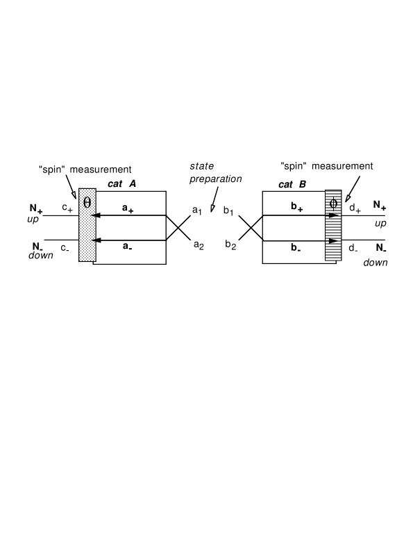
FIG. 1.: Arrangement to demonstrate that Schrödinger cats $A$ and $B$ defy a macroscopic reality. The number $N_{+}$ of particles (intensity) polarised “up” is either macroscopically larger (result $+1$), or macroscopically smaller (result $-1$), than $N_{+}$, the number of particles (intensity) polarised “down”.

The detection of the fields $\hat{c}_{\pm}$ allows determination of the total number $N_{+}^{A}=\hat{c}^{\dagger}_{+}\hat{c}_{+}$, of particles in the transmitted $up$ direction for $A$, and the total number of particles, $N_{-}^{A}=\hat{c}^{\dagger}_{-}\hat{c}_{-}$, in the orthogonal or $down$ direction for $A$. Our measurement on cat $A$ is of the particle number difference

$$2\hat{S}_{z}^{A}(\theta)=N_{+}^{A}-N_{-}^{A}=\hat{c}^{\dagger}_{+}\hat{c}_{+}-\hat{c}^{\dagger}_{-}\hat{c}_{-}$$ (2)

where using the Schwinger representation we have a direct equivalence to spin measurements. For measurement on cat $B$ we have similar definitions $\hat{d}_{+}={\bf\hat{b}_{+}}\cos(\phi/2)+{\bf\hat{b}_{-}}\sin(\phi/2)$ and $\hat{d}_{-}={\bf\hat{b}_{+}}\sin(\phi/2)-{\bf\hat{b}_{-}}\cos(\phi/2)$. The particle number difference for cat $B$ is $2\hat{S}_{z}^{B}(\phi)=N_{+}^{B}-N_{-}^{B}$ where $N_{+}^{B}=\hat{d}^{\dagger}_{+}\hat{d}_{+}$ and $N_{-}^{B}=\hat{d}^{\dagger}_{-}\hat{d}_{-}$.

It is necessary that the fields, our “cats”, be macroscopic states, of large particle or photon number. This experiment, with a macroscopic number of particles incident on the polarisers, is then a macroscopic version of the original Bell inequality experiment${}^{\cite[cite]{[\@@bibref{Number}{7}{}{}]}}$, the original Bell proposal involving only one particle incident on each polariser (or spin analyser). While such macroscopic Bell experiments have been examined previously${}^{\cite[cite]{[\@@bibref{Number}{12,13,14,15}{}{}]}}$ by Mermin, Peres and others, it is an crucial requirement of our experiment that the relevant outcomes for both blue ($\theta,\phi$) and green ($\theta^{\prime},\phi^{\prime}$) measurements, on both cats, are macroscopically distinct.

As with Schrodinger’s original gedanken experiment, we propose to generate (Figure 1) the macroscopic state, for ${\bf\hat{a}_{\pm}}$ and ${\bf\hat{b}_{\pm}}$, from a microscopic quantum state $|\psi\rangle$ for two field modes $\hat{a}_{1}$ and $\hat{b}_{1}$. We require that this original state be entangled, and as one example we consider the circular superposition of coherent states${}^{\cite[cite]{[\@@bibref{Number}{16}{}{}]}}$

$$|\psi\rangle=N\int_{0}^{2\pi}|r_{0}e^{i\varsigma}\rangle_{a_{1}}|r_{0}e^{-i\varsigma}\rangle_{b_{1}}d\varsigma$$ (3)

where $r_{0}=1.1$, $N^{2}=e^{2r_{0}^{2}}/4\pi^{2}I_{0}(2r_{0}^{2})$ and $|{\gamma}\rangle_{k}$ is the coherent state for mode $k$. We introduce a second pair of macroscopic quantum fields $\hat{a}_{2}$ and $\hat{b}_{2}$, in coherent states $|\alpha\rangle_{a_{2}}$ and $|\beta\rangle_{b_{2}}$ respectively, where $\alpha$, $\beta$ are real and large. Fields $\hat{a}_{1},\hat{a}_{2}$ are combined (using beam splitters or polarisers) to give macroscopic fields ${\bf\hat{a}_{-}}=(\hat{a}_{1}-\hat{a}_{2})/\sqrt{2}$ and ${\bf\hat{a}_{+}}=i(\hat{a}_{1}+\hat{a}_{2})/\sqrt{2}$ incident on the polariser for $A$. Similarly $\hat{b}_{1},\hat{b}_{2}$ are mixed to give macroscopic outputs ${\bf\hat{b}_{\pm}}$ for $B$. The systems being measured, the fields ${\bf\hat{a}_{\pm}},{\bf\hat{b}_{\pm}}$ incident on the polarisers, are macroscopic. The total size of the system $A$ is $\hat{S}_{A}=N_{+}^{A}+N_{-}^{A}=\hat{a}^{\dagger}_{1}\hat{a}_{1}+\hat{a}^{\dagger}_{2}\hat{a}_{2}$, which as $\alpha\rightarrow\infty$ is dominated by the Poissonian probability distribution mean $\alpha^{2}$. The fields ${\bf\hat{a}_{+}},{\bf\hat{a}_{-}}$ are individually similarly macroscopic with mean photon number $\alpha^{2}/2$.

We choose to write this macroscopic state $|\Psi\rangle$ using as a basis (the Pointer basis) the eigenstates $|m\rangle,|n\rangle,|S_{A}\rangle,|S_{B}\rangle$ of the measured quantities $2\hat{S}_{z}^{A}(\theta)=N_{+}^{A}-N_{-}^{A}$, $2\hat{S}_{z}^{B}(\phi)=N_{+}^{B}-N_{-}^{B}$, $\hat{S}_{A}=N_{+}^{A}+N_{-}^{A}$, $\hat{S}_{B}=N_{+}^{B}+N_{-}^{B}$ respectively. This is done by noting $\hat{c}_{+}=i(\hat{a}_{1}\exp(-i\theta/2)+\hat{a}_{2}\exp(i\theta/2))/\sqrt{2}$ and $\hat{c}_{-}=(-\hat{a}_{1}\exp(-i\theta/2)+\hat{a}_{2}\exp(i\theta/2))/\sqrt{2}$.

$$|\Psi\rangle = \sum_{m,n=-\infty}^{\infty}\sum_{S_{A},S_{B}}A(m,n,S_{A},S_{B})|m\rangle|n\rangle|S_{A}\rangle|S_{B}\rangle$$ (4)

Values for $S_{A},S_{B}$ must ensure positive $\hat{c}^{\dagger}_{\pm}\hat{c}_{\pm}$, $\hat{d}^{\dagger}_{\pm}\hat{d}_{\pm}$. The joint probability $P(m,n)$ of outcome $m,n$, for measurements $N_{+}^{A}-N_{-}^{A}$, $N_{+}^{B}-N_{-}^{B}$, is $P(m,n)=\sum_{S_{A},S_{B}}|A(m,n,S_{A},S_{B})|^{2}$. Results show complete symmetry between positive and negative $m$ values: $A(-m,n,S_{A},S_{B})=A(m,n,S_{A},S_{B})$; also for $n$. The crucial point is that for any fixed but arbitrary, positive $N_{0}$, the amplitude $A(m,n,S_{A},S_{B})$ where $-N_{0}\leq m,n\leq N_{0}$ can be made arbitrarily small by increasing $\alpha,\beta$. In this way we obtain a superposition of states with $m<N_{0}$ and states with $m>N_{0}$. This is true for all choices of basis $\theta,\phi$, and as $N_{0}$ becomes large we have a multi-faceted (blue and green) Schrodinger-cat state${}^{\cite[cite]{[\@@bibref{Number}{17}{}{}]}}$. Importantly the cat-state is prepared prior to the choice of measurement angles $\theta,\phi$.

To give our proposed definitive proof of the Schrodinger cat we demonstrate that in the asymptotic limit, $\alpha,\beta\rightarrow\infty$, we have two macroscopically distinct outcomes for measurements $S_{z}^{A}(\theta)$ (and $S_{z}^{B}(\phi)$), yet can still violate the Bell inequality (2). Consider three regions of outcome: first, where the result $m$ for the particle number difference $N_{+}-N_{-}$ satisfies $m>N_{0}$, result designated $1$; second, where $m<-N_{0}$ (result $-1$); and third, $-N_{0}\leq m\leq N_{0}$ (result $0$). For $N_{0}$ macroscopic, the outcomes $1$ and $-1$ are macroscopically distinct in particle number $m$. For arbitrarily large, fixed $N_{0}$, the probability of result $0$, $\sum_{m=-N_{0}}^{N_{0}}\sum_{n=-\infty}^{\infty}P(m,n)$, becomes increasingly negligible as $\alpha,\beta\rightarrow\infty$, while a clear violation of our inequality (1) in this asymptotic limit is maintained, at $E=2.03$${}^{\cite[cite]{[\@@bibref{Number}{18}{}{}]}}$ (Figure 2).

Plots of the probability distribution $P(m,n)$ do indeed reveal the asymptotic macroscopic limit where the shape of the distribution is unchanged. This final asymptotic shape $P_{a}(x,y)$ is dependent only on $x=m/\alpha,y=n/\beta$. As $\alpha=\beta$ increase, this probability function moves outward along the photon number $m$ and $n$ axes.

The macroscopic asymptotic limit can be checked analytically by expanding the operators for the coherent fields${}^{\cite[cite]{[\@@bibref{Number}{9}{}{}]}}$ as $\hat{a}_{2}=\alpha+\delta\hat{a}_{2}$. In the large $\alpha,\beta$ limit leading terms are $2\hat{S}_{z}^{A}(\theta)\sim\alpha\hat{X}_{\theta}^{A}$ (similarly $2\hat{S}_{z}^{B}(\phi)\sim\beta\hat{X}_{\phi}^{B}$). The quadrature phase amplitudes $\hat{X}_{\theta}^{A}=\hat{a}_{1}\exp(-i\theta)+\hat{a}_{1}^{\dagger}\exp(i\theta)$ and $\hat{X}_{\phi}^{B}=\hat{b}_{1}\exp(-i\phi)+\hat{b}_{1}^{\dagger}\exp(i\phi)$ are linear combinations of the “position” and “momentum” variables of the harmonic oscillators $\hat{a}_{1}$, $\hat{b}_{1}$, respectively. Our measurement

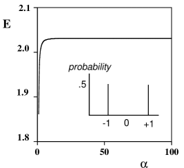
FIG. 2.: Quantum prediction of $E$ versus $\alpha=\beta$, with $\theta=0,\phi=-\pi/4,\theta^{\prime}=\pi/2,\phi^{\prime}=-3\pi/4$. The inset shows the probabilities, for all choices of $\theta$, and $\phi$, of obtaining results $-1$,$0$, and $+1$, at $A$ or $B$, in the large $\alpha,\beta$ limit.

$2\hat{S}_{z}^{A}(\theta)$ in Figure 1 for large $\alpha$ is operationally equivalent to the balanced homodyne detection measurement${}^{\cite[cite]{[\@@bibref{Number}{19}{}{}]}}$ of $\hat{X}_{\theta}^{A}$, except that here all fields are macroscopic prior to the selection of the measurement angle $\theta$. The asymptotic form, $P_{a}(x,y)$, of $P(m,n)$ coincides with the distribution (derived in [20]) for the results $x$, $y$ of measurements $\hat{X}_{\theta}^{A}$, $\hat{X}_{\phi}^{B}$ respectively, where $m\rightarrow\alpha x$, $n\rightarrow\beta y$. In the macroscopic limit the probability of outcome $0$ becomes $\int_{-\delta_{0}}^{\delta_{0}}dx\int_{-\infty}^{\infty}P_{a}(x,y)dy=\epsilon$ where $N_{0}=\alpha\delta_{0}$. We can make this probability less than or equal to a pre-specified arbitrarily small value $\epsilon$, by determining $\delta_{0}$ from the asymptotic form $P_{a}(x,y)$, and choosing $\alpha\geq N_{0}/\delta_{0}$.

There is analogy with the Schrödinger gedanken experiment: a coupling of the entangled microscopic state $|\psi\rangle$ to ${\hat{a}_{2}},\hat{b}_{2}$ generates the macroscopic entangled state (4) (the cats). Subsequent photon number measurements on these cats reveal a macroscopic entanglement through the violation of the macroscopic Bell inequalities (1). This macroscopic entanglement evident in $m,n$ directly reflects the original continuous variable entanglement, evident in $x,y$, of $|\psi\rangle$${}^{\cite[cite]{[\@@bibref{Number}{10}{}{}]}}$.

With this insight we predict that any state $|\psi\rangle$ demonstrating a failure of Bell’s premise of local realism, for such continuous variable (amplitude or position and momentum) measurements, will violate the macroscopic realism-locality premise we define here. A number of such entangled states have been recently predicted${}^{\cite[cite]{[\@@bibref{Number}{20,21,22}{}{}]}}$ and are of increasing interest because of potential applications to the field of quantum information${}^{\cite[cite]{[\@@bibref{Number}{19,23}{}{}]}}$.

This experiment would then not seem impossible. Quantum states satisfying our criteria are two-mode equivalents to the coherent superposition states $\sim(|\alpha_{0}\rangle\pm|-\alpha_{0}\rangle)/\sqrt{2}$, the subject of much experimental interest, for small $\alpha_{0}$${}^{\cite[cite]{[\@@bibref{Number}{3,4,5}{}{}]}}$. As with balanced homodyne detection the photon number difference is measured by taking the difference of two currents generated from highly efficient photodiode detectors. The measurement apparatus is a simple modification of that proposed${}^{\cite[cite]{[\@@bibref{Number}{24}{}{}]}}$ and used experimentally${}^{\cite[cite]{[\@@bibref{Number}{19}{}{}]}}$ in the realization of the continuous variable Einstein-Podolsky-Rosen paradox${}^{\cite[cite]{[\@@bibref{Number}{25}{}{}]}}$. We note that the quantum prediction could also apply to massive particles such as bosonic atoms.

REFERENCES

- [1] E. Schrödinger, Naturwissenschaften 23, 807 (1935).
- [2] J. R. Friedman, V. Patel, W. Chen, S. K. Tolpygo and J. E. Lukens, Nature 406, 43-45 (2000).
- [3] C. Monroe, D. M. Meekhof, B. E. King and D. J. Wineland. Science, 272, 1131 (1996).
- [4] M. W. Noel and C. R. Stroud, Phys. Rev. Lett., 1913 (1996).
- [5] M. Brune, E. Hagley, J. Dreyer, X. Maitre, A. Maali, C. Wunderlich, J. M. Raimond and S. Haroche. Phys. Rev. Lett., 77, 4887 (1996).
- [6] F. De Martini, V. Mussi and F. Bovino, Opt. Commun. 17, 581 (2000); presented at Europe IQEC (2000). See also F. De Martini, Phys. Rev. Lett. 81, 2842 (1998).
- [7] J. S. Bell, “Speakable and Unspeakable in Quantum Mechanics” (Cambridge Univ. Press, Cambridge, 1988). A. Aspect, P. Grangier and G. Roger, Phys. Rev. Lett. 49, 91, (1982). D. M. Greenberger, M. A. Horne, A. Shimony and A. Zeilinger, Am. J. Phys. 58, 1131 (1990).
- [8] A. J. Leggett and A. Garg, Phys. Rev. Lett. 54, 857 (1985).
- [9] M. D. Reid, Phys. Rev. Lett, 84, 2765 (2000); Phys. Rev. A. 62, 022110 (2000).
- [10] The measurements , are noncommuting: in the Schwinger representation; there is no contradiction with an uncertainty principle here, since becomes large in particle number; .
- [11] In the event of a violation of (1), it might be proposed that the macroscopic realism-locality premise fails because of an interaction of the local measurement procedure with the cat state. This possibility can be precluded because, as with the microscopic case, (1) is derivable assuming such interactions.
- [12] N. D. Mermin, Phys. Rev. D 22, 356 (1980); Phys. Rev. Lett. 65, 1838 (1990)
- [13] P. D. Drummond, Phys. Rev. Lett. 50, 1407 (1983).
- [14] S. L. Braunstein and C. M. Caves, 61, 662 (1988).
- [15] A. Peres, Phys. Rev. A 46, 4413 (1992); Found. Phys. 22,1819 (1992).
- [16] G. S. Agarwal, Phys. Rev. Lett. 57, 827-829 (1986). M. D. Reid and L. Krippner, Phys. Rev. A47, 552, (1993).
- [17] While the distinction between our states is small relative to the overall size of the system, the absolute value of this distinction can be as large as we specify.
- [18] Violations of a related premise, macroscopic local realism, are discussed in [9].
- [19] Z. Y. Ou, S. F. Pereira, H. J. Kimble and K. C. Peng, Phys. Rev. Lett. 68, 3663 (1992); Yun Zhang, Hai Wang, Xiaoying Li,Jietai Jing, Changde Xie and Kunchi Peng, Phys. Rev. A 62, 023813 (2000); Ch. Silberhorn, P. K. Lam, G. Wasik, N. Korolkova and G. Leuchs, presented at Europe IQEC (2000).
- [20] A. Gilchrist, P. Deuar and M. D. Reid, Phys. Rev. Lett. 80, 3169 (1998); Phys. Rev. A 60, 4259 (1999).
- [21] B. Yurke, M. Hillery and D. Stoler. Phys. Rev. A 60, 3444 (1999). M. Hillery, B. Yurke and D. Stoler, to be published.
- [22] W. J. Munro and G. J. Milburn, Phys. Rev. Lett. 81, 4285 (1998); W. J. Munro, Phys. Rev. A 59, 4197 (1999).
- [23] L. Vaidmann, Phys. Rev. A 49, 1473 (1994). S. Braunstein and H. J. Kimble, Phys. Rev. Lett. 80, 869 (1998). A. Furasawa, J. Sorensen, S. Braunstein, C. Fuchs, H. Kimble and E. Polzik, Science 282, 706 (1998).
- [24] M. D. Reid, Phys. Rev. A 40, 913 (1989).
- [25] A. Einstein, B. Podolsky and N. Rosen, Phys. Rev. 47, 777, (1935).