#2

DEBRECENI EGYETEM

TERMÉSZETTUDOMÁNYI KAR
Continued fraction representation of quantum mechanical Green’s operators
Ph.D. thesis

by

Balázs Kónya
University of Debrecen
Faculty of Sciences
Debrecen, 2000

Ez a dolgozat a Magyar Tudományos Akadémia Atommagkutató Intézete Elméleti Fizika Osztályán készült 2000-ben. A dolgozat alapjául szolgáló eredmények illetve tudományos közlemények a MTA ATOMKI Elméleti Fizika Osztályán és a Karl–Franzens Universität Graz Elméleti Fizika Intézetében születtek 1997. és 2000. között.

Ezen értekezést a Debreceni Egyetem fizika doktori program magfizika alprogramja keretében készítettem 1997. és 2000. között és ezúton benyújtom a Debreceni Egyetem doktori Ph.D. fokozatának elnyerése céljából. Debrecen, 2000. április 20. Kónya Balázs

Tanúsítom, hogy Kónya Balázs doktorjelölt 1997. és 2000. között a fent megnevezett doktori alprogram keretében irányításommal végezte munkáját. Az értekezésben foglaltak a jelölt önálló munkáján alapulnak, az eredményekhez önálló alkotó tevékenységével meghatározóan hozzájárult. Az értekezést elfogadásra javaslom. Debrecen, 2000. április 20. Dr. Papp Zoltán témavezető

Debrecen – 2000

Preface

This thesis contains the summary of my research work carried out as a Ph.D. student at the Theoretical Physics Department of the Institute of Nuclear Research of the Hungarian Academy of Sciences Debrecen, Hungary and partly at the Theoretical Physics Institute of the Karl-Franzens Universität Graz within the framework of the fruitful collaboration between the few-body research groups of Debrecen and Graz. The new results underlying this thesis have already been presented at international scientific meetings and published in four papers appeared in Journal of Mathematical Physics and Physical Review C. [31, 32, 33, 34].

As the title “Continued fraction representation of quantum mechanical Green’s operators” implies my research work is concerned with one of the central concepts of quantum mechanical few-body problems. The exploitation of the richness of the mathematical theory of continued fractions has enabled us to develop a rather general method for evaluating an analytic and readily computable representation of Green’s operators. This effective representation facilitates the solution of fundamental few-body integral equations.

Being a theoretical physicist I have always been interested in mathematics. Therefore as a second year undergraduate physics student I was enthusiastic to accept the research task on two-point Padé approximants offered by my present supervisor. Later under his supervision I finished my diploma work on the second order Dirac equation. By the time of my PhD studies I got completely infected with mathematical physics and my attention was attracted to the topic of continued fractions and quantum mechanics. During my work I benefitted a lot from my supervisor’s knowledge and experience, and I could identify myself with many of his thoughts. He showed me how mathematics could be used in practice approaching real physical problems. I hope my thesis may serve as an example for how physics has always profited from mathematics.

Here I would like to take the occasion and thank to everybody who helped me during the time I did my research and wrote my thesis.

Special thanks go to Prof. Zoltán Papp my PhD supervisor for his guidance and useful advises and for the excellent atmosphere in which we have been working together.

Some of the work covered by this thesis was done and the results were published together with Dr. G. Lévai. I thank him for the efforts he invested in our common topic. This collaboration was a very instructive experience for me, I could learn from him how one could always be optimistic even in the most hopeless moments.

I am grateful to the Theoretical Physics Department of ATOMKI for providing me a peaceful and pleasant working environment. I thank Prof. Borbála Gyarmati, who read the manuscript and made numerous helpful suggestions. I am indebted to Prof. R. G. Lovas who made the completion of my thesis possible by offering a young research fellow scholarship.

I am also grateful to the few-body group of the Theoretical Physics Institute of the Karl-Franzens Universität Graz, especially to Prof. W. Plessas, for the vivid scientific atmosphere.

Last but not least I wish to thank all the Professors of the Tuesday and Thursday 4PM open-air seminars for their brilliant lectures on tactics, sport diplomacy and football.

Contents

1. Preface
2. 1 Introduction
3. 2 The quantum mechanical Green’s operator
   1. 2.1 Definition
   2. 2.2 Basic properties of Green’s operator
   3. 2.3 The Green’s operator in scattering theory
   4. 2.4 Dunford–Taylor integrals of Green’s operators
4. 3 Tridiagonal matrices, recurrence relations and continued fractions
   1. 3.1 Infinite tridiagonal matrices
   2. 3.2 Three-term recurrence relations
   3. 3.3 Continued fractions
      1. 3.3.1 Analytic continuation of continued fractions
      2. 3.3.2 Pincherle’s theorem
5. 4 Continued fraction representation of …
   1. 4.1 The method
   2. 4.2 D-dimensional Coulomb Green’s operator
      1. 4.2.1 Convergence of the continued fraction
      2. 4.2.2 Numerical test
   3. 4.3 Relativistic Coulomb Green’s operators
      1. 4.3.1 Relativistic energy spectrum
   4. 4.4 D-dimensional harmonic oscillator
   5. 4.5 The generalized Coulomb potential
      1. 4.5.1 The potential
      2. 4.5.2 The matrix elements of the Green’s operator
6. 5 Applications
   1. 5.1 Model nuclear potential calculation
      1. 5.1.1 Bound states
      2. 5.1.2 Resonance states
      3. 5.1.3 Scattering states
      4. 5.1.4 Conclusions
   2. 5.2 An atomic three-body problem
      1. 5.2.1 Faddeev–Merkuriev integral equations
      2. 5.2.2 Solution in Coulomb–Sturmian space representation
7. Summary
8. Összefoglalás (The Hungarian summary of the thesis.)
9. References

Chapter 1 Introduction

The theoretical description of the microscopic world can be approached following two “orthogonal” paths. According to the many-body or field theoretical approach the microscopic world is considered as an assembly of many or infinitely many interacting objects, where field theoretical or statistical methods can be applied in order to describe the system [1, 2, 3]. On the contrary, few-body physicist tackle physical systems possessing only few degrees of freedom being consisted of a couple of interacting particles and intend to provide a physically complete and mathematically well formulated description.

Few-body systems have played a crucial role in the development of our understanding of microscopic world: atomic, nuclear and particle physics heavily rely on few-body models. Nowadays however, few-body problem has an ambiguous reputation of being a jungle where non-experts are quickly discouraged and specialist enjoy endless debates on technical improvements concerning equations and mathematical physics issues. Furthermore much attention has been paid only to computational consequences and little concern about the underlying physics. This is of course a false impression which originates from the non-trivial nature of the problems studied. The goal of the few-body physics community, namely giving a complete and mathematically correct description of few-body systems, automaticly requires the consideration of mathematical issues, hence this field offers an excellent playground for mathematical physics. This thesis, following the above ideas, hopes to contribute to the magnificent results achieved by the few-body approach.

Microscopic few-body physics certainly was born together with quantum mechanics in the pioneering work of Bohr, Heisenberg and Schrödinger trying to describe simple quantum systems, like the Hydrogen atom. The field initially developed as a part of nuclear physics as the title of the first few-body conference (Nuclear forces and the few-nucleon problem [4] held in London 1959) suggests. Since then few-body physics has expanded to incorporate atomic, molecular and quark systems. For example, the two-electron atom had already been attacked by Hylleraas [5] in 1929 and conquered by Pekeris [6] only in 1959. The theoretical foundations of few-body quantum physics were laid down by Lippmann and Schwinger [7], Gell-mann and Goldberger [8] by developing formal scattering theory of two-particle systems. The first attempts to extend the results to multichannel processes and more than two particles led to unsound mathematical formalism and non-unique solutions. The rigorous theory of few-body systems was given by Faddeev [9] who proposed a set of coupled integral equations which have a unique solution for the three-body problem. Having the correct few-body theory much effort has been invested into the development of numerical methods. The first numerical solution of the Faddeev equations for three spinless particles interacting with local potentials was achieved by Humberston at al. [10] in 1968. Since then a lot has been achieved due to the unbelievable development in computational power and the several extremely effective new methods having been developed. Among others, configuration and momentum space Faddeev calculations [11, 12, 13], the hyperspherical harmonics expansion method [14], the quantum Monte Carlo method [15], the Coulomb–Sturmian discrete space Faddeev approach [16] and the stochastic variational method [17] have been used to study few-body bound, resonant and scattering phenomena with great success.

The fundamental equations governing the dynamics of few-body physical systems, like the Lippmann–Schwinger equation and the Faddeev equations, are formulated in terms of integral equations. Integral equation formalism has a great advantage over the equivalent traditional differential equations because of the few-body boundary conditions are automatically incorporated into the integral equations. This is the reason why integral equation methods are in favour when scattering problems with complicated asymptotic behaviour are considered. Nevertheless for cases, where the asymptotics of the wave function is well known, differential equation approach can perform outstandingly (see i.e. the stochastic variational method [17]).

In spite of the fundamental merits of integral equations, their use in practical calculations is usually avoided and various approximations to the few-body Schrödinger equation are preferred instead. The reason for this is certainly that the integral equations contain not the usual Hamiltonian operator, but its resolvent, the Green’s operator in their kernel. The evaluation of the Green’s operator is much more complicated than the direct treatment of the Hamiltonian using standard tools of theoretical and mathematical physics. The determination of the Green’s operator is equivalent to the solution of the problem characterized by the corresponding Hamiltonian. In standard textbooks on quantum mechanics [18] Green’s operators are introduced on the level of fundamental equations and their general properties are extensively studied. Formal scattering theory [19, 20], thus few-body quantum mechanics can be formulated upon the notion of Green’s operator. The Green’s operator, similarly to the wave function, carries all the information of the physical system. Consequently the determination of the Green’s operator, as the central concept of few-body quantum mechanics, is of extreme importance.

The suitable choice of the Hilbert space representation can facilitate the determination of the Green’s operator. In this respect the momentum space representation is rather appealing as the free Green’s operator is extremely simple there. This is the main reason why momentum space techniques are so frequently used and also why they are capable of coping with complicated integral equations (for a review see [12]). On the other hand the use of discrete Hilbert space basis representation is often very advantageous because it transforms the integral equations into matrix equations. The harmonic oscillator (HO) functions [21] and the Coulomb–Sturmian (CS) functions are good examples of discrete Hilbert space basises. The free Green’s operator can also be given analytically between harmonic oscillator states [22]. This allowed the construction of a flexible method [23, 24] for solving the Lippmann-Schwinger equation, which contains the free Green’s operator in its kernel and provides a solution with correct free asymptotics in HO space. The CS basis representation of the Coulomb Green’s operator in terms of well computable special functions was derived by Papp in Ref. [25], where he could perform complicated analytic integrals of the Coulomb Green’s function and the Coulomb–Sturmian functions making use of the results of Ref. [26].

The CS representation of the Coulomb Green’s operator forms the basis of a quantum mechanical approximation method developed recently [25, 27, 28] for describing Coulombic systems. The strength of the method is that the Coulomb–like interactions in the two-body calculations are treated asymptotically correctly, since the Coulomb Green’s operator is calculated analytically and only the asymptotically irrelevant short-range interaction is approximated. This way the correct Coulomb asymptotics is guaranteed. The corresponding computer codes for solving two-body bound, resonant and scattering state problems were also published [29]. The method has been extended to solve the three-body Coulomb problem in the Faddeev approach. In this formulation of the Faddeev equations the most crucial point is to calculate the resolvent of the sum of two independent, thus commuting two-body Coulombic Hamiltonian. This resolvent is given as a convolution integral of two-body Green’s operators. Therefore the evaluation of the contour integral requires the analytic knowledge of the two-body Green’s operators. So far good results have been obtained by Papp for bound state [16] and for below-breakup scattering state three-body problems [30].

In practice there is no general procedure for how to determine Hilbert space representation of a Green’s operator. All the Green’s operators mentioned before require separate and detailed investigation sometimes based on very specific considerations. In a recent publication [31] we have proposed a rather general and easy-to-apply method for calculating discrete Hilbert space basis representation of Green’s operators belonging to some class of Hamiltonians. We have shown that if in some basis representation the Hamiltonian possesses an infinite symmetric tridiagonal (Jacobi) matrix structure, the corresponding Green’s operator can be given in terms of a continued fraction. The procedure necessitates the analytic calculation of the matrix elements of the Hamiltonian as the only input in the analytic evaluation of the Green’s matrix in terms of a convergent continued fraction. This method simplifies the determination of Green’s matrices considerably and the representation via continued fraction provides a readily computable and numerically stable Green’s matrix. The Green’s operator of the non-relativistic two-body Coulomb problem and the D-dimensional harmonic oscillator problem was evaluated utilizing this method in Ref. [31]. An exactly solvable potential problem, which provides a smooth transition between the Coulomb and the harmonic oscillator problem, was considered in Ref. [32]. A suitable basis was defined in which the Hamiltonian of the potential problem appeared in tridiagonal form. With the help of the analytically calculated matrix elements of the Hamiltonian the determination of the Green’s matrix was straightforward. The Hamiltonian of the radial Coulomb Klein–Gordon and second order Dirac equation was shown to possess infinite symmetric tridiagonal structure in the relativistic CS basis. This again allowed us to give an analytic representation of the corresponding relativistic Coulomb Green’s operators in terms of continued fraction [33]. The continued fraction representation of the Coulomb Green’s operator was utilized to give a unified description of bound, resonant and scattering states of a model nuclear potential [34] using a quantum mechanical approximation method [23] devised to solve the Lippmann–Schwinger equation.

The layout of this thesis is the following:
This introductory chapter is followed by a chapter devoted to the concept of the Green’s operator. Here few-body quantum theory is built up around the Green’s operator. In Chapter 3 a review of tridiagonal matrices, three-term recurrence relations and continued fractions is given. The method of calculating continued fraction representation of certain class of Green’s operators is presented in Chapter 4. This chapter also covers the calculation of continued fraction representation of the D-dimensional Coulomb, D-dimensional harmonic oscillator, the generalized Coulomb and the relativistic Coulomb Green’s operators. In the last chapter two typical applications of the Green’s operator in few-body physics are delivered. First the continued fraction representation of Coulomb Green’s operator is used to present a unified description of bound, resonant and scattering states of a model nuclear potential demonstrating the central role of Green’s operators in few-body quantum mechanics. Then the binding energy of the Helium atom is calculated by solving the Faddeev–Merkuriev equations for the atomic three-body problem in Coulomb–Sturmian Hilbert space representation. Chapter 4 and 5 contain the new results of the author. Finally, summary and bibliography closes the thesis.

Chapter 2 The quantum mechanical Green’s operator

Expressions like Green’s operator, Green’s function and propagator are frequently used in different fields of physics and mathematics sometimes with confusing meanings. For example the many-body Green’s function $G_{\alpha\beta}(xt,x^{\prime}t^{\prime})$ studied in quantum many-body problem is defined as the ground state expectation value of fields operators in the second quantized formalism [1]. Whereas the propagator of relativistic quantum field theory is often referred to as the Green’s function as well [2, 3].

The Green’s operator of few-body quantum physics corresponds to the definition of mathematical physics [35].

2.1 Definition

Suppose $H$ is a Hermitian differential operator in some Hilbert space. The $G(z)$ Green’s operator is defined as the resolvent operator of $H$

$$G(z)(z-H)=(z-H)G(z)={\bf 1}\qquad\mbox{for}\quad z\in{\mathbb{C}}/\sigma(H),$$ (2.1)

where $\sigma(H)$ denotes the spectrum of the Hermitian operator $H$ and ${\bf 1}$ is the identity operator. So, the $G(z)=(z-H)^{-1}$ Green’s operator is defined on the whole complex plane ${\mathbb{C}}$ except for the spectrum of $H$.

The $\{|r\rangle\}$ coordinate basis representation of the (2.1) operator equation

$$\delta(r-r^{\prime})=\langle r|{\mathrm{I}}|r^{\prime}\rangle, \quad\int\mbox{dr}|r\rangle\langle r^{\prime}|={\bf 1}$$ (2.2)

$$G(r,r^{\prime};z)=\langle r|G(z)|r^{\prime}\rangle, \quad\delta(r-r^{\prime})H(r)=\langle r|H|r^{\prime}\rangle$$ (2.3)

leads to an inhomogeneous differential equation

$$[z-H(r)]G(r,r^{\prime};z)=\delta(r-r^{\prime})$$ (2.4)

for $G(r,r^{\prime};z)$. In mathematical physics the Green’s function corresponding to the linear Hermitian differential operator $H(r)$, where $r\in\Omega$, and to the complex variable $z$ is defined as the solution of the inhomogeneous equation (2.4) subject to certain boundary conditions for $r,r^{\prime}$ on the surface of the domain $\Omega$. In fact the Green’s function is required to satisfy the same boundary condition as the wave function. Consequently the $G(r,r^{\prime};z)$ Green’s function of mathematical physics can be viewed as the coordinate space representation of the $G(z)$ resolvent operator.

In what follows, under the notion of few-body Green’s operator the (2.1) resolvent of the Hamiltonian is to be understood. In the next chapters Hilbert space basis representation of Green’s operators will be investigated.

2.2 Basic properties of Green’s operator

The determination of the Green’s operator represents the solution of the underlying differential equation. Therefore the evaluation of the Green’s operator corresponding to the Hamiltonian $H$ is equivalent to the complete description of the system characterized by $H$. The Green’s operator carries all the information about the physical system. Once some representation of $G(z)$ is known one can gain the eigenvalues and the eigenfunctions of the Hamiltonian, construct projection operators or determine the density of states, etc,. The time evaluation operator can also be obtained by performing a Fourier transform of the Green’s operator.

Let $\{|\phi_{n}\rangle\}$ and $\{\alpha_{n}\}$ denote the complete set of orthonormal eigenstate and the corresponding eigenvalues of the Hermitian operator $H$

$$H|\phi_{n}\rangle=\alpha_{n}|\phi_{n}\rangle\ .$$ (2.5)

Utilizing the completeness of the eigenstates, the Green’s operator can be written as

$$G(z)=\sum_{n}\frac{|\phi_{n}\rangle\langle\phi_{n}|}{z-\alpha_{n}}+\int\mbox{dn}\frac{|\phi_{n}\rangle\langle\phi_{n}|}{z-\alpha_{n}},$$ (2.6)

where $\sum_{n}$ and $\int\mbox{dn}$ indicates summation over the discrete and the continuous spectrum, respectively.

Since $H$ is Hermitian, all of its $\alpha_{n}$ eigenvalues are real, which means that $G(z)$ is an analytic function in the complex $z$-plane except at those points and intervals of the real axis which corresponds to the spectrum of $H$. According to (2.6) $G(z)$ possesses simple poles at the positions of the discrete eigenvalues of $H$, hence the poles of $G(z)$ give the discrete energy eigenvalues of the Hamiltonian. The residue at the $\alpha_{n}$ pole provides information on the corresponding non-degenerate $|\phi_{n}\rangle$ eigenvector according to the projection operator

$$|\phi_{n}\rangle\langle\phi_{n}|=\frac{1}{2\pi\mbox{i}}\oint_{\alpha_{n}}dz\ G(z),$$ (2.7)

here the contour encircles the $\alpha_{n}$ and only the $\alpha_{n}$ eigenvalue. Equation (2.7) can be used to construct the wave function.

If $\lambda\in{\mathbb{R}}$ belongs to the continuous part of the spectrum, then $G(\lambda)$ is usually defined by a non-unique limiting procedure

$$G^{+}(\lambda):=\lim_{\epsilon\to 0^{+}}G(\lambda+i\epsilon)$$ (2.8)

$$G^{-}(\lambda):=\lim_{\epsilon\to 0^{+}}G(\lambda-i\epsilon)$$ (2.9)

because of the existence of the limits. Thus the continuum spectrum of $H$ appears as a singular line (branch cut) of $G(z)$. Due to the self-adjointness of the Hamiltonian the Green’s operator exhibits the important property

$$G(z^{*})=G(z)^{*}\ .$$ (2.10)

Therefore $G^{+}(\lambda)$ and $G^{-}(\lambda)$ are connected by

$$G^{-}(\lambda)=\left(G^{+}(\lambda)\right)^{*},$$ (2.11)

from which we have

$${\mbox{R}e}G^{-}(\lambda)={\mbox{R}e}G^{+}(\lambda),\quad{\mbox{I}m}G^{-}(\lambda)=-{\mbox{I}m}G^{+}(\lambda)\ .$$ (2.12)

The knowledge of ${\mbox{R}e}G^{\pm}(\lambda)$ allows us to obtain the density of states at $\lambda$

$$\Delta(\lambda)=\mp\frac{1}{\pi}{\mbox{I}m}\{Tr[G^{\pm}(\lambda)]\}\ .$$ (2.13)

The time development of the $|\psi(t_{0})\rangle$ state belonging to the Hamiltonian $H$ at $t=t_{0}$ can be obtained as a solution of the time dependent Schrödinger equation, and it is governed by the $U(t,t_{0})$ time evolution operator according to

$$|\psi(t)\rangle=U(t,t_{0})|\psi(t_{0})\rangle,$$ (2.14)

where the time evolution operator

$$U(t,t_{0})=e^{-\frac{i}{\hbar}H(t-t_{0})}$$ (2.15)

can be expressed in terms of the Green’s operator as

$$U(t,t_{0})=i\hbar\int_{-\infty}^{\infty}\frac{{\mbox{d}\omega}}{2\pi}e^{-i\omega(t-t_{0})}\left[G^{+}(\hbar\omega)-G^{-}(\hbar\omega)\right]$$ (2.16)

Equation (2.16) shows that the $U(t,t_{0})$ propagator can be determined as the Fourier transform of the $G^{\pm}$ Green’s operators.

2.3 The Green’s operator in scattering theory

The formulation of quantum scattering theory is heavily relied on the concept of Green’s operator. It is concerned with the mathematical description of the scattering process during which the incident beam of particles, usually prepared by some accelerator, enters into interaction in the scattering region then the scattered beam is observed by detectors located at large distance from the interaction area.

Far from the scattering region the incoming and the scattered beam can be thought of as bunch of particles propagating freely, therefore they can be characterized by the $|\psi_{in}\rangle$, $|\psi_{out}\rangle$ asymptotic states whose time evolution are governed by the $H^{0}$ asymptotic Hamiltonian as

$$|\psi_{in/out}(t)\rangle=U_{0}(t)|\psi_{in/out}(t_{0})\rangle,\quad U_{0}(t)=e^{-\frac{i}{\hbar}H^{0}t}.$$ (2.17)

On the other hand the time evolution of the scattering process is fully determined by the $H=H^{0}+V$ total Hamiltonian involving the scattering potential as well:

$$|\psi(t)\rangle=U(t)|\psi(t_{0})\rangle,\quad U(t)=e^{-\frac{i}{\hbar}Ht},$$ (2.18)

here $|\psi(t)\rangle$ denotes the actual scattering state vector. However, during scattering experiments one can only measure the $|\psi_{in}\rangle$ incoming and the $|\psi_{out}\rangle$ outgoing asymptotes of $|\psi\rangle$. Therefore in scattering theory all information about the scattering process should be extracted from the asymptotic behavior of $|\psi\rangle$.

At $t=0$ let $|\phi+\rangle$ ($|\chi-\rangle$) denotes the $|\psi(t)\rangle$ scattering state which evolved from the $|\psi_{in}\rangle=|\phi\rangle$ incoming asymptote (evolved to the $|\psi_{out}\rangle=|\chi\rangle$ outgoing asymptote). The $|\phi+\rangle$ and $|\chi-\rangle$ scattering states are related to their asymptotes by the equations

$$|\phi+\rangle = \Omega_{+}|\phi\rangle$$ (2.19)

$$|\chi-\rangle = \Omega_{-}|\chi\rangle,$$

where the $\Omega_{\pm}$ Møller operators are defined as the limits of the time evolution operators

$$\Omega_{\pm}=\lim_{t\to\mp\infty}U(t)^{\dagger}U^{0}(t).$$ (2.20)

The existence of the Møller operator can be proved if the scattering potential satisfies certain conditions (i.e. not too singular at the origin, sufficiently short ranged and smooth, see [20]). The main goal of the scattering description is to relate the outgoing asymptote to the incoming one without reference to the experimentally unknown actual orbit. Utilizing the $\Omega_{-}^{\dagger}\Omega_{-}={\bf 1}$ isometric property of the Møller operator from Eq. (2.19) we obtain

$$|\psi_{out}\rangle=\Omega_{-}^{\dagger}\Omega_{+}|\psi_{in}\rangle:=S|\psi_{in}\rangle,$$ (2.21)

here $S:=\Omega_{-}^{\dagger}\Omega_{+}$ is the scattering operator, which carries all the experimentally important information about the scattering. Once the operator $S$ is determined the scattering problem is solved.

In order to determine the $S$ operator it is convenient to use the $\{|\vec{p}\rangle\}$ momentum representation. It is important to note here that the $|\vec{p}\rangle$ plane wave momentum eigenstates do not represent physically realizable states, in fact they are only used in the expansion of physical states of the scattering process as

$$|\psi\rangle=\int{\mathrm{d}^{3}p}\ \psi(\vec{p})|\vec{p}\rangle.$$ (2.22)

Similarly the scattering state $|\phi+\rangle$ can be expressed as

$$|\phi+\rangle=\Omega_{+}|\phi\rangle=\int{\mathrm{d}^{3}p}\ \phi(\vec{p})\Omega_{+}|\vec{p}\rangle=\int{\mathrm{d}^{3}p}\ \phi(\vec{p})|\vec{p}+\rangle,$$ (2.23)

where the $|\vec{p}+\rangle=\Omega_{+}|\vec{p}\rangle$ improper (i.e. not normalizable) vector is called the stationary scattering vector corresponding to the $|\vec{p}\rangle$ incoming plane wave.

In momentum representation a careful mathematical analysis leads to the very important result

$$\begin{split}\Omega_{+}|\phi\rangle&=|\phi+\rangle=\lim_{t\to-\infty}U(t)^{\dagger}U_{0}(t)|\phi\rangle\\ &=|\phi\rangle+i\int_{0}^{-\infty}\mbox{d}\tau\ U(\tau)^{\dagger}VU^{0}(\tau)|\phi\rangle\\ &=|\phi\rangle+i\lim_{\epsilon\to 0^{+}}\int_{0}^{-\infty}\mbox{d}\tau\ e^{+\epsilon\tau}U(\tau)^{\dagger}VU^{0}(\tau)|\phi\rangle\\ &=|\phi\rangle+i\lim_{\epsilon\to 0^{+}}\int{\mathrm{d}^{3}p}\ G(E_{p}+i\epsilon)V|\vec{p}\rangle\left<\vec{p}|\phi\right>\end{split}$$ (2.24)

which establishes the connection between the $\Omega_{+}$ Møller and the $G^{+}(z)$ Green’s operator. After expanding $|\phi+\rangle$ and $|\phi\rangle$ in Eq. (2.24) in terms of the improper states $|\vec{p}\rangle$ and $|\vec{p}+\rangle$ we obtain for the stationary scattering vector $|\vec{p}\pm\rangle$

$$|\vec{p}\pm\rangle=|\vec{p}\rangle+\lim_{\epsilon\to 0^{+}}G(E_{p}\pm i\epsilon)V|\vec{p}\rangle\ .$$ (2.25)

Making use of the

$$A^{-1}=B^{-1}+B^{-1}(B-A)A^{-1}$$ (2.26)

operator identity with $A=z-H$ and $B=z-H^{0}$, then with their interchange, we can derive the

$$G(z)=G^{0}(z)+G^{0}(z)VG(z)$$ (2.27)

$$G(z)=G^{0}(z)+G(z)VG^{0}(z)$$

resolvent equations, which relate the $G^{0}$ and the $G$ operators. With these equations Eq. (2.25) can be recast in the form

$$|\vec{p}\pm\rangle=|\vec{p}\rangle+\lim_{\epsilon\to 0^{+}}G^{0}(E_{p}\pm i\epsilon)V|\vec{p}\pm\rangle.$$ (2.28)

This type of integral equations were first formulated by Lippmann and Schwinger [7], consequently Eq. (2.27) and Eq. (2.28) are known as the Lippmann–Schwinger equations for $G$ and $|\vec{p}\pm\rangle$, respectively. According to (2.25) and (2.28) the evaluation of the stationary scattering vectors necessitates the determination of the full Green’s operator or the solution of the (2.28) Lippmann–Schwinger equation.

Being able to calculate $|\vec{p}\pm\rangle$, one can obtain any scattering information. For example, the $\langle\vec{p}^{\>\prime}|S|\vec{p}\rangle$ scattering matrix can be written as

$$\langle\vec{p}^{\>\prime}|S|\vec{p}\rangle=\delta_{3}(\vec{p}^{\>\prime}-\vec{p})-2\pi i\delta(E_{p^{\prime}}-E_{p})\ t(\vec{p}^{\>\prime}\leftarrow\vec{p}).$$ (2.29)

Here $t(\vec{p}^{\>\prime}\leftarrow\vec{p})$ can be calculated using the $|\vec{p}\pm\rangle$ scattering states

$$t(\vec{p}^{\>\prime}\leftarrow\vec{p})=\langle\vec{p}^{\>\prime}|V|\vec{p}+\rangle=\langle\vec{p}^{\>\prime}\!-|V|\vec{p}\rangle,$$ (2.30)

or using the Green’s operator

$$t(\vec{p}^{\>\prime}\leftarrow\vec{p})=\langle\vec{p}^{\>\prime}|V+VGV|\vec{p}\rangle.$$ (2.31)

The $(V+VGV)$ operator is called the $T$ operator. Its $t(\vec{p}^{\>\prime}\leftarrow\vec{p})$ matrix element is referred to as the on-shell $T$ matrix, because in Eq. (2.29) it appears together with the $\delta(E_{p^{\prime}}-E_{p})$ delta function, and thus defined only for the ${p^{\prime}}^{2}=p^{2}$ "on-shell" energy case.

The experimentally off important differential scattering cross section $d\sigma/d\Omega$ can be derived from the (2.29) formula for the scattering matrix, and has the form

$$\frac{d\sigma}{d\Omega}=|f(\vec{p}^{\>\prime}\leftarrow\vec{p})|^{2},$$ (2.32)

where $f(\vec{p}^{\>\prime}\leftarrow\vec{p})$ is the scattering amplitude, which is just a trivial factor times the on-shell $T$ matrix

$$f(\vec{p}^{\>\prime}\leftarrow\vec{p})=-(2\pi)^{2}m\ t(\vec{p}^{\>\prime}\leftarrow\vec{p}).$$ (2.33)

Finally we quote here the asymptotic form of the coordinate representation of the stationary scattering vector

$$\lim_{r\to\infty}\left<\vec{r}|\vec{p}+\right>=(2\pi)^{-\frac{3}{2}}\left[e^{i\vec{p}\vec{r}}+f(p\hat{r}\leftarrow\vec{p})\frac{e^{ipr}}{r}\right],$$ (2.34)

which reflects the traditional definition of scattering states as the sum of an incident plane wave and a spherically spreading scattered wave, whose $f(p\hat{r}\leftarrow\vec{p})$ amplitude determines the scattering cross section via (2.32).

In this short review it was demonstrated that the knowledge of the Green’s operator enables one to determine the scattering states, which is equivalent to the solution of the scattering problem and makes possible the calculation of any scattering quantities.

2.4 Dunford–Taylor integrals of Green’s operators

From the theory of linear operators [36] we know that the analytic function of a bounded self-adjoint operator $A$ can be defined as the Dunford–Taylor integral representation

$$f(A)=\frac{1}{2\pi\mathrm{i}}\oint_{C}dz\;f(z)(z-A)^{-1},$$ (2.35)

where $C$ encircles the spectrum of $A$ in positive direction and $f$ should be analytic on the domain encircled by $C$. This definition can be considered as the operator equivalent of the Cauchy integral formula.

In few-body physics one often encounters the problem of determining Green’s operators corresponding to Hamiltonians composed of two independent operators with known resolvents. This is the typical situation when the Green’s operator of separable subsystems are known (e.g. think of a three-dimensional motion decomposed to the sum of a two- and a one-dimensional motion). The question, whether it is possible to determine the Green’s operator of the composite system making use of the sub-Green’s operators naturally emerges. The answer can be given by utilizing the (2.35) Dunford–Taylor integral representation.

Let $h_{1},h_{2}$ be two independent (hence commuting) bounded linear operators with the analytically known $g_{1}(z)=(z-h_{1})^{-1}$, $g_{2}(z)=(z-h_{2})^{-1}$ resolvents. Then applying the (2.35) definition for $f(\lambda)=(z-h_{1}-\lambda)^{-1}$ and $A=h_{2}$, the $G(z)=(z-H)^{-1}$ Green’s operator of the $H=h_{1}+h_{2}$ composite Hamiltonian can be evaluated by performing a convolution integral of the $g_{1}(z)$, $g_{2}(z)$ sub-Green’s operators

$$G(z)=\frac{1}{2\pi\mbox{i}}\oint_{C}dz^{\prime}\,g_{1}(z-z^{\prime})\;g_{2}(z^{\prime}),$$ (2.36)

where the contour $C$ should encircle, in counterclockwise direction, the spectrum (discrete and continuous) of $h_{2}$ without penetrating into the spectrum of $h_{1}$. In Fig. 2.1 a typical integration scenario in the complex $z^{\prime}$-plane is shown for a bound state system ($z<0$). We note that among others, Bianchi and Favella [37] proposed a convolution integral of the type of (2.36) for determining the resolvent of the sum of two commuting Hamiltonian.

The (2.35) integal representation can also be used to construct other well-known operators as a Dunford–Taylor integral of the Green’s operator. For example, the identity operator

$$1=\frac{1}{2\pi\mbox{i}}\oint_{C}dz\>\>(z-h)^{-1},$$ (2.37)

the Hamilton operator

$$h=\frac{1}{2\pi\mbox{i}}\oint_{C}dz\>z\>(z-h)^{-1}\ ,$$ (2.38)

or the time evolution operator

$$\exp(-\mbox{i}ht)=\frac{1}{2\pi\mbox{i}}\oint_{C}dz\>\exp(-\mbox{i}zt)\>(z-h)^{-1}$$ (2.39)

can be given as analytic integrals of the $g=(z-h)^{-1}$ Green’s operator.

Figure 2.1: The integration path $C$ in the complex $z^{\prime}$-plane for the convolution integral of the (2.36) Green’s operator.

Chapter 3 Tridiagonal matrices, recurrence relations and continued fractions

Based on the mathematical literature [39, 40, 41, 42] this chapter is dedicated to the survey of the mathematical machinery being used in the forthcoming part of the thesis. First a truncated inverse of an infinite symmetric tridiagonal matrix is presented. Tridiagonal matrices inherently imply three-term recurrence relations for the matrix elements of their inverse. For this reason the basic properties of three-term recurrence relations are outlined. The final section discusses the fundamentals of the theory of continued fractions. The analytic continuation and an important type of transformation of continued fractions is investigated. The intimate relation of continued fractions and three-term recurrence relations is revealed by Pincherle’s theorem.

3.1 Infinite tridiagonal matrices

Infinite rank matrices naturally emerge in quantum mechanics when physical observables are represented on a discrete infinite dimensional basis. Moreover the matrix representation of many physical operators are tridiagonal in a certain basis. In fact, some computational methods, like the Lanczos method [43, 39], are based on the scheme of creating a basis that renders a given Hamiltonian tridiagonal. However we are always limited to consider finite rank truncations of infinite matrices. Here we derive a formula [31] for the n-th leading submatrix of the inverse of an infinite symmetric tridiagonal matrix. The underlying idea originally came up in the work of Pál [44], and we give here the proof.

Let $A:=[a_{ij}],\>i,j=1,2,\ldots,\infty$, be an infinite symmetric tridiagonal (Jacobi) matrix:

$$a_{ii-1}=\beta_{i-1},\quad a_{ii}=\alpha_{i},\quad a_{ii+1}=\beta_{i},\quad a_{ij}=0\quad\mbox{for}\quad|i-j|>1.$$ (3.1)

Let $B:=[b_{ij}],\>i,j=1,2,\ldots,\infty$ denote the infinite rank matrix, for which

$${\bf 1}=AB=BA,\quad\delta_{ij}=\sum_{k=1}^{\infty}a_{ik}b_{kj}.$$ (3.2)

Then the following theorem can be stated.

Theorem 1.

Let us define the $n$-th leading submatrices of $A$ and of $B$ as
$A_{n}:=[a_{ij}]$, $B_{n}:=[b_{ij}],\>i,j=1,2,\ldots,n$, respectively. Then

$$B_{n}=(A_{n}+F_{n})^{-1},$$ (3.3)

where $F_{n}:=[f_{ij}],\quad i,j=1,\ldots,n$, is given by

$$f_{ij}=\left\{\begin{array}[]{ll}0&\quad i,j<n\\ 0&\quad i=n,j<n\\ 0&\quad j=n,i<n\\ a_{nn+1}\frac{\displaystyle b_{1n+1}}{\displaystyle b_{1n}}&\quad i=j=n\end{array}\right.$$ (3.4)

Proof of Theorem 1.

Utilizing the (3.1) tridiagonal property of $A$, the (3.2) definining relation of $B$ for $i,j\leq n$ can be written as

$$\delta_{ij}=\sum_{k=1}^{n}a_{ik}b_{kj}+\delta_{in}a_{nn+1}b_{n+1j},\quad i,j\leq n,$$ (3.5)

which we can rewrite in the form

$$\delta_{ij}=\sum_{k=1}^{n}\left(a_{ik}b_{kj}+\delta_{in}a_{in+1}b_{n+1j}\delta_{kn}\frac{b_{kj}}{b_{nj}}\right)=\sum_{k=1}^{n}\left(a_{ik}+\delta_{in}\delta_{kn}a_{in+1}\frac{b_{n+1j}}{b_{nj}}\right)b_{kj}.$$ (3.6)

The inverse of a symmetric tridiagonal matrix possesses the following property [40]:

$$b_{ij}=\left\{\begin{array}[]{r@{\quad\mbox{if}\quad}l}p_{i}q_{j},&i\leq j\\ p_{j}q_{i},&j\leq i\end{array}\right..$$ (3.7)

Therefore

$$\frac{b_{n+1j}}{b_{nj}}=\frac{p_{j}q_{n+1}}{p_{j}q_{n}}=\frac{p_{1}q_{n+1}}{p_{1}q_{n}}=\frac{b_{1n+1}}{b_{1n}},$$ (3.8)

and follows the statement of the theorem:

$$\delta_{ij}=\sum_{k=1}^{n}\left(a_{ik}+\delta_{in}\delta_{kn}a_{in+1}\frac{b_{1n+1}}{b_{1,n}}\right)b_{kj}=\sum_{k=1}^{n}(a_{ik}+f_{ik})b_{kj}.\quad$$ (3.9)

∎

Finally we give a schematic picture of the theorem. The infinite symmetric tridiagonal matrix $A$ and its n-th leading submatrix $A_{n}$ can be illustrated as

$$A=\left(\begin{array}[]{cccc}A_{n}&\cdot&&\\ \cdot&\cdot&\cdot&\\ &\cdot&\cdot&\cdot\\ &&\cdot&\cdot\end{array}\right)_{\infty\bf{x}\infty}\quad A_{n}=\left(\begin{array}[]{cccc}\cdot&\cdot&&\\ \cdot&\cdot&\cdot&\\ &\cdot&\cdot&\cdot\\ &&\cdot&\cdot\end{array}\right)_{n\times n}$$ (3.10)

Similarly the infinite $B$ and the truncated $B_{n}$ general matrices can be plotted

$$B=\left(\begin{array}[]{cccc}B_{n}&\cdot&\cdot&\cdot\\ \cdot&\cdot&\cdot&\cdot\\ \cdot&\cdot&\cdot&\cdot\\ \cdot&\cdot&\cdot&\cdot\end{array}\right)_{\infty\bf{x}\infty}\quad B_{n}=\left(\begin{array}[]{cccc}\cdot&\cdot&\cdot&\cdot\\ \cdot&\cdot&\cdot&\cdot\\ \cdot&\cdot&\cdot&\cdot\\ \cdot&\cdot&\cdot&\cdot\end{array}\right)_{n\times n}$$ (3.11)

With the above schematic representation of matrices, the (3.3) statement of Theorem 1 can be recast in the form

$$\left(\begin{array}[]{cccc}\cdot&\cdot&\cdot&\cdot\\ \cdot&\cdot&\cdot&\cdot\\ \cdot&\cdot&\cdot&\cdot\\ \cdot&\cdot&\cdot&\cdot\end{array}\right)_{n\times n}=\left[\left(\begin{array}[]{cccc}\cdot&\cdot&&\\ \cdot&\cdot&\cdot&\\ &\cdot&\cdot&\cdot\\ &&\cdot&\cdot\end{array}\right)_{n\times n}+\left(\begin{array}[]{cccc}&&&\\ &&&\\ &&&\\ &&&f_{n,n}\end{array}\right)_{n\times n}\right]^{-1}\$$ (3.12)

where $f_{nn}=a_{nn+1}b_{1n+1}/b_{1n}$.

According to Eq. (3.12) the truncated inverz $B_{n}$ is readily calculable from the $a_{ij}$ tridiagonal matrix elements, provided the $b_{1n+1}/b_{1n}$ quotient is at our disposal.

3.2 Three-term recurrence relations

Due to Eq. (3.2) the matrix elements $b_{ij}$ of the inverz of an infinite symmetric tridiagonal matrix automatically satisfy a three-term recurrence relation in both indexes

$$\delta_{ij}=\beta_{i-1}b_{i-1j}+\alpha_{i}b_{ij}+\beta_{i}b_{i+1j},\quad\mbox{for}\quad i=1,\ldots,\infty,\quad j\;\mbox{fixed},$$ (3.13)

$$\delta_{ij}=\beta_{j-1}b_{ij-1}+\alpha_{j}b_{ij}+\beta_{j}b_{ij+1},\quad\mbox{for}\quad j=1,\ldots,\infty,\quad i\;\mbox{fixed}.$$ (3.14)

Let us consider the (homogeneous) three-term recurrence relation

$$x_{n+1}=b_{n}x_{n}+a_{n}x_{n-1},\quad a_{n}\neq 0,\qquad n=1,2,3,\ldots,$$ (3.15)

where $a_{n},b_{n}$ complex numbers are the coefficients of the recurrence relation. A sequence of complex numbers $\{x_{n}\}^{\infty}_{n=0}$ is called a solution of (3.15) if its $x_{n}$ elements satisfy the equation for all $n\in{\mathbf{N}}$. The set of all solutions $\{x_{n}\}^{\infty}_{n=0}$ of (3.15) form a linear vector space of dimension two over the field of complex numbers, and the zero vector of this space is the $\{0\}^{\infty}_{n=0}$ trivial solution. A distinguished type of solution is the minimal solution. If there exists a non-trivial solution $\{m_{n}\}^{\infty}_{n=0}$ and another solution $\{d_{n}\}^{\infty}_{n=0}$ of (3.15) such that

$$\lim_{n\rightarrow\infty}\frac{m_{n}}{d_{n}}=0,$$ (3.16)

then $\{m_{n}\}$ is called the minimal (subdominal) solution. A solution which is not minimal, like $\{d_{n}\}$, is called the dominant solution. In general, a recurrence relation may or may not have a minimal solution, and it is clear that if $\{m_{n}\}$ is a minimal solution then $\{m^{\prime}\}:=c\{m\}$ for $\forall c\neq 0$ is a minimal solution as well. Moreover any other non-trivial $\{y_{n}\}$ solutions are dominant since they can be written

$$\{y_{n}\}=c_{1}\{m_{n}\}+c_{2}\{d_{n}\},\quad c_{2}\neq 0,$$ (3.17)

where $\{d_{n}\}$ is a dominant solution. The existence of a minimal solution is strongly related to the convergence of a continued fraction (see Section 3.3).

Suppose the $x_{0}$ and $x_{1}$ elements of the (3.15) three-term recurrence relation are at our disposal and we want to apply the recurrence relation in a direct way to determine $\{x_{n}\}_{n=0}^{\infty}$ recursively. However, for a minimal solution this method does fail in practice. Gautschi [45] pointed out that a direct recursive calculation of a minimal solution of a three-term recurrence relation is numerically unstable. A surprising demonstration of this instability can be found in [41] on page 219.

We note here that three-term linear recurrence relations are closely linked to linear difference equations of order two.

3.3 Continued fractions

The study of continued fractions, i.e. mathematical expressions of the form

$$b_{o}+\cfrac{a_{1}}{b_{1}+\cfrac{a_{2}}{b_{2}+\cfrac{a_{3}}{b_{3}+\cdots+\cfrac{a_{n}}{b_{n}}}}}$$ (3.18)

started in the 16th century with a work of Bombelli [46] in 1572, who wrote down the first finite continued fraction

$$3+\cfrac{4}{6+\cfrac{4}{6}}=3.6$$ (3.19)

to approximate $\sqrt{13}\approx 3.6055$. The traditional form (3.18) of a continued fraction is often written more economically as

$$b_{0}(z)+\frac{a_{1}}{b_{1}}{\atopwithdelims. .+}\frac{a_{2}}{b_{2}}{\atopwithdelims. .+}\frac{a_{3}}{b_{3}}{\atopwithdelims. .+}\cdots{\atopwithdelims. .+}\frac{a_{n}}{b_{n}}.$$ (3.20)

The first continued fractions were constructed from integers and were used to approximate various algebraic numbers, among others the $\pi$. From the 17th century on the continued fraction evolved into an important tool of number theory. First Schwenter, Huygens, Wallis latter Lagrange, Legendre, Gauss and Galois made extensive use of regular continued fractions, continued fractions with integer coefficients, in their number theoretical studies.

Euler extended the notion of a continued fraction by generalizing its coefficients as functions of complex variables rather than simple numbers. This way continued fraction expansions could be used as special tools in the analytic approximations of special classes of analytic functions. Following Euler’s results a long list of brilliant mathematicians from the 19th century, names like Laplace, Jacobi, Riemann, Stieltjes, Frobenius and Tchebycheff made flourish the analytic theory of continued fractions within the framework of the classical 19th century analysis.

Mathematical physics had also discovered the continued fractions. Continued fraction expansion of special functions, solution of three-term recurrence relations and Padé approximants represent important field of applications. The available continuously increasing computational power has also contributed to the present-day success of continued fractions in mathematical physics.

Rigorously a continued fraction is defined as an ordered pair of the type

$$((\{a_{n}(z)\},\{b_{n}(z)\}),\{f_{n}(z)\}),$$ (3.21)

where $\{a_{n}(z)\}_{1}^{\infty}$ and $\{b_{n}(z)\}_{0}^{\infty}$, with all $a_{n}(z)\neq 0$, are two sequences of complex valued functions defined on the region $D$ of the complex plane. The complex values of $a_{n}(z)$ and $b_{n}(z)$ are called the $n$-th partial numerator and partial denominator of the continued fraction, or simply the coefficients or elements. The $\{f_{n}(z)\}$ sequence of complex functions is given by

$$f_{n}(z)=S_{n}(0,z),\qquad n=0,1,2,\ldots,$$ (3.22)

where

$$S_{n}(w_{n},z)=S_{n-1}(s_{n}(w_{n},z),z),\qquad S_{0}(w_{0},z)=s_{0}(w_{0},z),$$ (3.23)

with the

$$s_{n}(w_{n},z)=\frac{a_{n}(z)}{b_{n}(z)+w_{n}},\quad n\geq 1,\qquad s_{0}(w_{0},z)=b_{0}(z)+w_{0},$$ (3.24)

linear fractional transformation.

Here $S_{n}(w_{n},z)$ is called the $n$-th approximant of the continued fraction with respect to the $\left\{w_{n}\right\}_{n=0}^{\infty}$ complex series. Applying recursively the (3.24) linear fractional transformation the $n$-th approximant of the continued fraction can be written as

$$S_{n}(w_{n},z)=b_{0}(z)+\frac{a_{1}(z)}{b_{1}(z)}{\atopwithdelims. .+}\frac{a_{2}(z)}{b_{2}(z)}{\atopwithdelims. .+}\cdots{\atopwithdelims. .+}\frac{a_{n}(z)}{b_{n}(z)+w_{n}}\ .$$ (3.25)

Similarly, for the $S_{n}(0,z)$ approximant we got

$$S_{n}(0,z)=b_{0}(z)+\mathop{K}_{i=1}^{n}\left(\frac{a_{i}(z)}{b_{i}(z)}\right)=b_{0}(z)+\frac{a_{1}(z)}{b_{1}(z)}{\atopwithdelims. .+}\frac{a_{2}(z)}{b_{2}(z)}{\atopwithdelims. .+}\cdots{\atopwithdelims. .+}\frac{a_{n}(z)}{b_{n}(z)},$$ (3.26)

where the new notation $\mathop{K}_{i=1}^{n}(a_{i}/b_{i})$ was introduced for the approximant. Subsequently for the $((\{a_{n}(z)\},\{b_{n}(z)\}),\{f_{n}(z)\})$ continued fraction one of the

$$b_{0}(z)+\frac{a_{1}(z)}{b_{1}(z)}{\atopwithdelims. .+}\frac{a_{2}(z)}{b_{2}(z)}{\atopwithdelims. .+}\cdots,\quad\mbox{or}\quad b_{0}(z)+\mathop{K}_{n=1}^{\infty}\left(\frac{a_{n}(z)}{b_{n}(z)}\right)$$ (3.27)

notations will be used.

The convergence of a continued fraction means the convergence of the sequence of approximants $S_{n}(w_{n},z)$ to an extended complex number

$$f(z)=\lim_{n\rightarrow\infty}S_{n}(w_{n},z)\ .$$ (3.28)

If $f(z)$ exists for two different sequences of $\{w_{n}\}$ then $f(z)$ is unique. For a detailed discussion of convergence results see Chapter IV of [42].

There are several algorithm to compute the $n$-th approximant of a continued fraction. The backward recurrence algorithm consists of summing-up the (3.25) fraction starting at its tail. This method is proved to be numerically stable. The main drawback of the backward recurrence algorithm is that it needs to be recalculated for each approximant. An alternative method, the forward recurrence algorithm is based upon the following

$$S_{n}(w_{n},z)=\frac{A_{n}(z)+A_{n-1}(z)w}{B_{n}(z)+B_{n-1}(z)w}$$ (3.29)

representation of $S_{n}(w_{n},z)$, where $A_{n}(z),B_{n}(z)$ are called the $n$-th numerator, denominator, respectively. The $n$-th numerator and denominator satisfy a recurrence relation namely

$$A_{n}(z)=b_{n}(z)+A_{n-1}(z)+a_{n}(z)A_{n-2}(z)$$ (3.30)

$$B_{n}(z)=b_{n}(z)+B_{n-1}(z)+a_{n}(z)B_{n-2}(z),$$ (3.31)

with $A_{-1}=1,A_{0}=b_{0},B_{-1}=0,B_{0}=1$. In contrast with the forward algorithm, one can easily obtain $S_{n+1}(w_{n+1},z)$ from $S_{n}(w_{n},z)$ using the backward algorithm, but on the other hand, this method is less stable than the first one.

A special class of continued fractions for which the limits

$$\lim_{n\rightarrow\infty}a_{n}(z)=a(z)\qquad\text{and}\qquad\lim_{n\rightarrow\infty}b_{n}(z)=b(z)$$ (3.32)

exist for all $z\in D$ is called the limit 1-periodic continued fraction. The more general case is the limit-k periodic continued fraction for which we have

$$\lim_{n\rightarrow\infty}a_{kn+p}(z)=a_{p}(z)\quad\text{and}\quad\lim_{n\rightarrow\infty}b_{kn+p}(z)=b_{p}(z)\quad\mbox{for}\quad p=1,2,\ldots,k\ .$$ (3.33)

Limit periodic continued fractions play an important role in the analytic theory of continued fractions, since most of the continued fraction representation of special functions are limit periodic continued fractions. The convergence properties of limit periodic continued fractions are determined by the behavior of their tail by means of the $w_{\pm}(z)$ fixed points of the limit linear fractional transformation

$$s(w,z)=\lim_{n\rightarrow\infty}s_{n}(w_{n},z)=\frac{a(z)}{b(z)+w}.$$ (3.34)

The $w_{\pm}(z)$ fixed points are given as the solutions of the $s(w)=w$ fixed point equation

$$w=\frac{a(z)}{b(z)+w}\quad\Rightarrow\quad w_{\pm}(z)=-b(z)/2\pm\sqrt{(b(z)/2)^{2}+a(z)}.$$ (3.35)

The fixed point with smaller modulus is called attractive fixed point, while the other one is named as the repulsive one. Since $w_{\pm}(z)$ represent the tail of a limit 1-periodic continued fraction we can accelerate the convergence using the attractive fixed point in the approximant $S_{n}(w,z)$ [47].

3.3.1 Analytic continuation of continued fractions

The idea of analytic continuation of a continued fraction $b_{0}(z)+\mathop{K}(a_{n}(z)/b_{n}(z))$ by means of an appropriate choice of $w_{n}(z)$ for the $S_{n}(w_{n}(z))$ approximant was proposed by Waadeland [48] and later recalled by Masson [49]. By examining limit periodic continued fractions they sought a modification of the tail of a continued fraction which led to its analytic extension.

If a continued fraction converges in a certain complex region $D$, then in many cases it is possible to extend the region of convergence to a larger domain $D^{*}\supseteq D$, where $D^{*}$ depends on the choice of the functions $w_{n}(z)$.

In the case of limit 1-periodic continued fractions the analytic continuation $f_{D^{*}}(z)$ of the continued fraction $f(z)$ in (3.28) is defined with the help of the fixed points $w_{\pm}(z)$ of Eq. (3.35) as

$$f_{D^{*}}(z)=\lim\limits_{n\to\infty}S_{n}(w_{\pm}(z),z).$$ (3.36)

In Eq. (3.36) the analytic expressions for the $w_{\pm}(z)$ fixed points are continued analytically and then employed to sum up the continued fraction, this way providing the analytic continuation of the continued fraction.

Bauer–Muir transformation

The numerical computation of approximants $S_{n}(w_{\pm}(z),z)$ might be unstable, specially for $z$ belonging to the extended region, which leads to unsatisfactory convergence. This problem can be overcome by using the Bauer–Muir transformation of a continued fraction (see eq. [41]) We note that the method dates back to the original work of Bauer [50] and Muir [51] in the 1870’s.

The Bauer–Muir transform of a continued fraction $b_{0}(z)+K\left(a_{n}(z)/b_{n}(z)\right)$ with respect to a sequence of complex numbers $\left\{w_{n}\right\}_{n=0}^{\infty}$ is defined as the continued fraction $d_{0}(z)+K\left(c_{n}(z)/d_{n}(z)\right)$, whose “classical” approximants $S_{n}(0,z)$ are equal to the modified approximants $S_{n}(w_{n},z)$ of the original continued fraction. The transformed continued fraction exists and can be calculated as

$$d_{0} = b_{0}+w_{0},\quad c_{1}=\lambda_{1},\quad d_{1}=b_{1}+w_{1},$$ (3.37)

$$c_{i} = a_{i-1}q_{i-1,}\quad d_{i}=b_{i}+w_{i}-w_{i-2}q_{i-1},\quad i\geq 2,$$

$$\lambda_{i} = a_{i}-w_{i-1}(b_{i}+w_{i}),\quad q_{i}=\lambda_{i+1}/\lambda_{i}\quad i\geq 1,$$

if and only if $\lambda_{i}\neq 0$ for $i=1,2,\ldots.$

3.3.2 Pincherle’s theorem

Continued fractions and three-term recurrence relations are intimitaly connected. The existence of a minimal solution of a (3.15) three-term recurrence relation is strongly related to the convergence of a continued fraction constructed from the coefficients of the recurrence relation. This connection is revealed by Pincherle in 1894 [52]. Below we state Pincherle’s theorem without its proof which can be found in [41, 42].

Theorem 2 (Pincherle’s Theorem).

Let $a_{n}$ and $b_{n}$ be a sequence of complex numbers with $a_{n}\neq 0$ for $n=1,2,\dots$
(A) The three-term recurrence relation

$$x_{n+1}=b_{n}x_{n}+a_{n}x_{n-1},\qquad n=1,2,3,\ldots,$$ (3.38)

with coefficients $a_{n}$ and $b_{n}$ has a minimal solution $\{m_{n}\}$ if and only if the continued fraction

$$\mathop{K}_{n=1}^{\infty}\left(\frac{a_{n}}{b_{n}}\right)=\frac{a_{1}}{b_{1}}{\atopwithdelims. .+}\frac{a_{2}}{b_{2}}{\atopwithdelims. .+}\cdots{\atopwithdelims. .+}\frac{a_{n}}{b_{n}}{\atopwithdelims. .+}\cdots$$ (3.39)

converges.
(B) Provided (3.38) has a minimal solution $\{m_{n}\}$, then for $N=0,1,2,\ldots,$

$$\frac{m_{N+1}}{m_{N}}=-K_{n=1}^{\infty}\left(\frac{a_{n+N}}{b_{n+N}}\right)=-\frac{a_{1+N}}{b_{1+N}}{\atopwithdelims. .+}\frac{a_{2+N}}{b_{2+N}}{\atopwithdelims. .+}\cdots{\atopwithdelims. .+}\frac{a_{n+N}}{b_{n+N}}{\atopwithdelims. .+}\cdots$$ (3.40)

Remarks:

• Equation (3.40) asserts that the ratio of two arbitrary successive elements of the minimal solution can be calculated by a continued fraction.

• The connection between continued fractions and three-term recurrence relations provides the link between continued fractions and special functions (i.e. hypergeometric functions and orthogonal polynomials).

• The genious Indian mathematican Ramanujan left behind, written in his notebook [53], many interesting and original contributions to modern mathematics among which several dealt with the theory of continued fractions. Unfortunately he did not give proofs of his ideas. It is worth noting that mathematicians have found Pincherle’s theorem as a useful tool to prove some of Ramanujan’s formulae.

Chapter 4 Continued fraction representation of Green’s operators

In this chapter we present a rather general and easy-to-apply method for calculating discrete Hilbert space basis representation of those Green’s operators that correspond to Hamiltonians having infinite symmetric tridiagonal (i.e. Jacobi) matrix form. The procedure necessitates the evaluation of the Hamiltonian matrix on this basis. The analytically calculated elements of the Jacobi matrix are used to construct a continued fraction, which is utilized in the evaluation of the Green’s matrix. The constructed continued fraction representation of the Green’s operator is convergent in the bound state energy region and can be continued analytically to the whole complex energy plane.

Our method of calculating Green’s matrices ensures a complete analytic and readily computable representation of the Green’s operator on the whole complex plane. Furthermore this is achieved at a very little cost: in practice only the matrix elements of the Hamiltonian are required.

After the expose of the method the continued fraction representation of specific Green’s operators are given. The Coulomb Green’s operator, relativistic Green’s operators, the Green’s operator corresponding to the D-dimensional harmonic oscillator and the Green’s operator of the generalized Coulomb potential is considered. The convergence and the analytic continuation of the continued fraction is illustrated with the example of the Coulomb Green’s operator. The numerical accuracy of the method is demonstrated via the calculation of the relativistic energy spectrum of hydrogen-like atoms.

4.1 The method

In order to determine a matrix representation of the Green’s operator, first a suitable basis has to be defined. Let us consider the set of states $\{|i\rangle\}$ and $\{|\tilde{i}\rangle\}$, with $i=0,1,2,\ldots$, which form a complete biorthonormal basis, i.e.

$$\langle\tilde{i}|j\rangle=\langle i|\tilde{j}\rangle=\delta_{ij}$$ (4.1)

$${\bf 1}=\sum_{i=0}^{\infty}|\tilde{i}\rangle\langle i|=\sum_{i=0}^{\infty}|i\rangle\langle\tilde{i}|$$

and render the $E-H$ operator symmetric tridiagonal

$${J}_{i^{\prime}i}=\langle i^{\prime}|(E-{H})|i\rangle=\left(\begin{array}[]{cccc}\cdot&\cdot&&\\ \cdot&\cdot&\cdot&\\ &\cdot&\cdot&\cdot\\ &&\cdot&\cdot\end{array}\right)_{\infty\times\infty}.$$ (4.2)

Here $E$ is a complex parameter and $H$ denotes the Hamilton operator. According to Eq. (4.2) we say that the Hamiltonian exhibits a Jacobi matrix structure.

The Green’s operator corresponding to the Hamiltonian ${H}$ satisfies the operator equation

$${\bf 1}={G}(E)(E-{H}).$$ (4.3)

In the (4.1) discrete biorthonormal basis representation this relation takes the form of the following matrix equation

$$\delta_{ji}=\sum_{i^{\prime}=0}^{\infty}\langle\tilde{j}|{G}(E)|\tilde{i}^{\prime}\rangle\langle i^{\prime}|(E-{H})|i\rangle=\sum_{i^{\prime}=0}^{\infty}G_{ji^{{}^{\prime}}}J_{i^{{}^{\prime}}i}.$$ (4.4)

Since the basis is chosen such that $E-H$ possesses a tridiagonal matrix representation, the Green’s matrix appears as the inverz of a symmetric infinite tridiagonal matrix.

In Section 3.1 the inverz of an infinite symmetric tridiagonal matrix was studied and a formula for its $n$-th leading submatrix was derived. Let us denote the $n$-th leading submatrix of the infinite Green’s matrix by $G^{(n)}$. According to Theorem 1, $G^{(n)}$ can be written as

$${G}_{ij}^{(n)}=\left[{J}_{ij}+\delta_{jn}\,\,\delta_{in}\,\,{J}_{nn+1}\,\,\frac{{G}_{0n+1}}{{G}_{0n}}\right]^{-1}\ .$$ (4.5)

Eq. (4.5) asserts that the Green’s matrix elements $G^{(n)}_{ij}$ can be calculated from the Jacobi matrix elements $J_{ij}$ provided the ${G}_{0n+1}/{G}_{0n}$ quotient is at our disposal.

On the other hand, from the tridiagonality of $E-H$ and from Eq. (4.4) it automatically follows that the matrix elements ${G}_{ji}=\langle\tilde{j}|{G}(E)|\tilde{i}\rangle$ satisfy a three-term recurrence relation

$$\delta_{ji}={G}_{ji-1}{J}_{i-1i}+{G}_{ji}{J}_{ii}+{G}_{ji+1}{J}_{i+1i}.$$ (4.6)

Therefore ${G}_{0n+1}/{G}_{0n}$ represents a ratio of two consecutive elements of a solution of a three-term recurrence relation. It is known, that the solutions of three-term recurrence relations span a two-dimensional space and a special type of solution, called the minimal solution, is intimately connected to continued fractions. (see Section 3.2 and 3.3). According to Pincherle’s Theorem, if the Green’s matrix elements represent a minimal solution of the (4.6) three-term recurrence relation, then the ratio of its two consecutive elements is given in terms of a convergent continued fraction

$$\frac{G_{0n+1}}{G_{0n}}=-\cfrac{u_{n}}{d_{n}+\cfrac{u_{n+1}}{d_{n+1}+\cfrac{u_{n+2}}{d_{n+2}+\cdots}}},$$ (4.7)

with coefficients

$$u_{i}=-\frac{J_{i,i-1}}{J_{i,i+1}},\quad d_{i}=-\frac{J_{i,i}}{J_{i,i+1}}.$$ (4.8)

The Green’s matrix elements $G_{ij}$ and the (4.6) three-term recurrence relation, by the (4.3) definition, obviously depend on the (complex) energy parameter $E$. First we show that there is a region of the complex $E$-plane where the physically relevant solution of the (4.6) recurrence relation for the Green’s matrix is the minimal one, which makes possible a convergent continued fraction representation of the Green’s operator on this region by utilizing Eqs. (4.5) and (4.7). Afterwards the analytic expression of the convergent continued fraction is extended to other domain of the $E$-plane, where the physical Green’s matrix is not the minimal solution of the recurrence relation.

On the $\Re E<0$ region of the complex plane and in case of short-range potentials the coordinate space representation of the Green’s operator can be constructed as [19]

$$G(r,r^{\prime},k)=\varphi_{l}(k,r_{<})f_{l}^{(+)}(k,r_{>})/{\cal F}(k),$$ (4.9)

where $\varphi_{l}(k,r)$ is the regular solution, ${\ f}_{l}^{(+)}(k,r)$ is the Jost solution, ${\cal F}(k)$ is the Jost function and $k$ is the wave number. The Jost solution is defined by the relation

$$\lim\limits_{r\to\infty}\mbox{e}^{\mp ikr}{\ f}_{l}^{(\pm)}(k,r)=1.$$ (4.10)

Let us define a “new” Green’s function as

$$\widetilde{G}(r,r^{\prime},k)=\varphi_{l}(k,r_{<})f_{l}(k,r_{>})/{\cal F}(k),$$ (4.11)

where $f_{l}$ is a linear combination of ${\ f}_{l}^{(+)}$ and ${\ f}_{l}^{(-)}$. If $\Re E<0$ ${\ f}_{l}^{(+)}$ is exponentially decreasing and ${\ f}_{l}^{(-)}$ is exponentially increasing. Thus, for any $\widetilde{G}$ we have

$$\lim\limits_{r^{\prime}\to\infty}\frac{G(r,r^{\prime},k)}{\widetilde{G}(r,r^{\prime},k)}=0,\qquad\mbox{if\ \ }\Re E<0.$$ (4.12)

We note, that both $G$ and $\widetilde{G}$ satisfy the defining equation Eq. (4.3), but only $G$ of Eq. (4.9) is the physical Green’s function. The above considerations, with a slight modification in Eq. (4.10), are also valid for the Coulomb case. An interesting result of the study of Ref. [54] is that the Green’s matrix from Jacobi-matrix Hamiltonian, has an analogous structure to Eq. (4.9)

$$G_{ii^{\prime}}(k)=({\varphi_{l}})_{i_{<}}(k)(f_{l}^{(+)})_{i_{>}}(k)/{\cal F}(k),$$ (4.13)

where $({\varphi_{l}})_{i}(k)=\langle\varphi_{l}(k)|\widetilde{i}\rangle$ and $(f_{l}^{(+)})_{i}(k)=\langle f_{l}^{(+)}(k)|\widetilde{i}\rangle$. Similarly, we define $(f_{l})_{i}(k)=\langle f_{l}(k)|\widetilde{i}\rangle$ and

$$\widetilde{G}_{ii^{\prime}}(k)=({\varphi_{l}})_{i_{<}}(k)(f_{l})_{i_{>}}(k)/{\cal F}(k).$$ (4.14)

On the $\Re E<0$ region of the complex plane as $r\to\infty$ $f_{l}(k,r)$ exponentially dominates over $f_{l}^{(+)}(k,r)$, thus for their $L^{2}$ representation the following relation holds

$$\lim\limits_{i\to\infty}\frac{(f_{l}^{(+)})_{i}(k)}{(f_{l})_{i}(k)}=0,\qquad\mbox{if\ \ }\Re E<0.$$ (4.15)

This implies a similar relation for the Green’s matrices

$$\lim\limits_{i^{\prime}\to\infty}\frac{G_{ii^{\prime}}(k)}{\widetilde{G}_{ii^{\prime}}(k)}=0,\qquad\mbox{if\ \ }\Re E<0.$$ (4.16)

So, we can conclude that in the $\Re E<0$ region of complex $E$-plane the physically relevant Green’s matrix $G_{ii^{\prime}}$ appears as the minimal solution of the (4.6) recurrence relation. Therefore our Green’s matrix for bound-state energies can be determined by a convergent continued fraction.

In other regions of the complex energy plane (i.e. the region of scattering energies and resonances) the continued fraction fails to converge and the recurrence relation does not have a minimal solution. On the other hand, $G_{0N+1}/G_{0N}$ in (4.7) is an analytic function of the complex energy parameter, and there is a domain of the complex plane where this function is represented by a convergent continued fraction, thus values on other domains can be obtained by the analytic continuation of a continued fraction (see Section 3.3.1).

Let us suppose we have a limit 1-periodic continued fractions, that is the $u_{i}$ and $d_{i}$ coefficients in (4.8) have the following limit property

$$\lim_{i\rightarrow\infty}u_{i}=u\hskip 8.5359pt\mbox{and}\ \lim_{i\rightarrow\infty}d_{i}=d.$$ (4.17)

In this case the continued fraction (4.7) takes the form

$$\cfrac{G_{0n+1}}{G_{0n}}=-\cfrac{u_{n}}{d_{n}+\cfrac{u_{n+1}}{d_{n+1}+\cdots+\cfrac{u}{d+\cfrac{u}{d+\cdots}}}}\ .$$ (4.18)

The $w$ tail of this continued fraction satisfies the implicit relation

$$w=\frac{u}{d+w}\ ,$$ (4.19)

which is solved by

$$w_{\pm}=-d/2\pm\sqrt{(d/2)^{2}+u}\ .$$ (4.20)

Replacing the tail of the continued fraction by its explicit analytic form $w_{\pm}$, we can speed up the convergence and, which is more important, we can perform an analytic continuation. This implies the usage of $w_{\pm}=w_{\pm}(z)$ in the (3.25) formula for the $S_{n}(w,z)$ continued fraction approximants also at those $z$ values, where the continued fraction fails to converge.

The $w_{+}$ choice gives an analytic continuation to the physical sheet, while $w_{-}$, which also converges, gives an analytic continuation to the unphysical sheet. This observation can be taken by considering the formula for the Green’s operator on the physical sheet [20]

$$\langle\widetilde{i}|G(E+\mbox{i}0)|\widetilde{i}\rangle-\langle\widetilde{i}|G(E-\mbox{i}0)|\widetilde{i}\rangle=-2\pi\mbox{i}\langle\widetilde{i}|\psi(E)\rangle\langle\psi(E)|\widetilde{i}\rangle,$$ (4.21)

where $\psi(E)$ is the scattering wave function, and utilizing the (2.11) analytic properties of Green’s operators. Then we can readily obtain that the imaginary part of $\langle\widetilde{i}|G(E+\mbox{i}0)|\widetilde{i}\rangle$ should be negative and this condition can only be fulfilled with the choice of $w_{+}$.

We have shown that Eqs. (4.5) and (4.7) together with the theory of analytic continuation of a continued fraction supply a complete discrete Hilbert space representation of the Green’s operator on the whole complex energy plane. The Green’s matrix can be obtained from the Jacobi Hamiltonian for arbitrary complex energies by simply evaluating a continued fraction and performing a matrix inversion.

4.2 D-dimensional Coulomb Green’s operator

Here we use the Coulomb–Sturmian basis and show that on this basis the D-dimensional Coulomb Hamiltonian possesses a Jacobi-matrix structure. Then the analytically derived $J$-matrix elements are utilized, following the method of the previous section, to calculate the continued fraction representation of the Green’s operator. The convergence of the continued fraction and the technique of the analytic continuation is demonstrated in practice.

Let us consider the $D$-dimensional radial Coulomb Hamiltonian

$$H^{\rm C}=-\frac{\hbar^{2}}{2m}\left(\frac{\mbox{d}^{2}}{\mbox{d}r^{2}}+\frac{1}{r^{2}}\left(l+\frac{D-3}{2}\right)\left(l+\frac{D-1}{2}\right)\right)+\frac{Z{\rm e}^{2}}{r}\ ,$$ (4.22)

where $m$, $l$, ${\rm e}$ and $Z$ stand for the mass, angular momentum, electron charge and charge number, respectively. (See, e.g. Ref. [55] and references.) The bound state energy spectrum is given by

$$E_{n_{r}l}=-\frac{mZ^{2}e^{4}}{2\hbar^{2}(n_{r}+l+\frac{D-1}{2})^{2}},$$ (4.23)

and the corresponding wave functions are

$$\psi_{n_{r}l}(r)=a_{0}\left(\frac{r_{0}\Gamma(n_{r}+1)}{2\Gamma(n_{r}+2l+D-1)}\right)^{1/2}\exp(-\frac{a_{0}}{2}r)(a_{0}r)^{l+\frac{D-1}{2}}L_{n_{r}}^{(2l+D-2)}(a_{0}r),$$ (4.24)

where we used the notation $a_{0}=((n_{r}+l+\frac{D-1}{2})r_{0})^{-1}$ and $r_{0}=\hbar^{2}/(2mZe^{2})$.

The Coulomb–Sturmian (CS) functions, the Sturm–Liouville solutions of the Hamiltonian (4.22), appear as

$$\phi_{nl}(b,r)=\left(\frac{\Gamma(n+1)}{\Gamma(n+2l+D-1)}\right)^{1/2}\exp(-br)(2br)^{l+\frac{D-1}{2}}L_{n}^{(2l+D-2)}(2br),$$ (4.25)

where $b$ is a scale parameter, $n$ is the radial quantum number and $L_{n}^{(\alpha)}$ denotes the generalized Laguerre polynomials [56]. The CS functions of (4.25) are the generalizations of the corresponding CS functions for the three-dimensional case [57]. Introducing the notation $\langle r|n\rangle\equiv\phi_{nl}(b,r)$ and $\langle r|\widetilde{n}\rangle\equiv\phi_{nl}(b,r)/r$ for the CS function and its biorthonormal partner respectively, we can express the orthogonality and completeness of these functions as

$$\langle n|\widetilde{n^{\prime}}\rangle=\delta_{nn^{\prime}}$$ (4.26)

$${\bf 1}=\sum_{n=0}^{\infty}|\widetilde{n}\rangle\langle n|=\sum_{n=0}^{\infty}|n\rangle\langle\widetilde{n}|,$$ (4.27)

confirming that they form a discrete biorthonormal basis in the sense of (4.1). The overlap of two CS functions can be written in terms of a three-term expression

$$\begin{split}\langle n|n^{\prime}\rangle=(2b)^{-1}\bigg{[}&+\delta_{nn^{\prime}}(2n+2l+D-1)\bigg{.}\\ &-\delta_{nn^{\prime}-1}((n+1)(n+2l+D-1))^{1/2}\\ &\bigg{.}-\delta_{nn^{\prime}+1}(n(n+2l+D-2))^{1/2}\bigg{]}.\end{split}$$ (4.28)

A similar expression holds for the matrix elements of $H^{C}$

$$\begin{split}\langle n|H^{C}|n^{\prime}\rangle=\frac{\hbar^{2}b}{4m}\bigg{[}&+\delta_{nn^{\prime}}\left(2n+2l+D-1-\frac{2}{r_{0}b}\right)\bigg{.}\\ &+\delta_{nn^{\prime}-1}((n+1)(n+2l+D-1))^{1/2}\\ &\bigg{.}+\delta_{nn^{\prime}+1}(n(n+2l+D-2))^{1/2}\bigg{]}.\end{split}$$ (4.29)

Let us denote the Coulomb Green’s operator as $G^{\rm C}(E)=(E-H^{\rm C})^{-1}$ and determine its CS matrix elements $G^{\rm C}_{ij}=\langle\widetilde{i}|G^{\rm C}_{l}|\widetilde{j}\rangle$ by applying the general method described previously. The starting point in this procedure is the observation that the $J_{ij}=\langle i|(E-H^{\rm C})|j\rangle$ matrix possesses an infinite symmetric tridiagonal i.e. Jacobi structure, and the nonzero elements of this tridiagonal matrix are obtained immediately from Eqs. (4.28) and (4.29) as

$$J_{ii} = (2i+2l+D-1)(k^{2}-b^{2})\frac{\hbar^{2}}{4mb}-Z{\rm e}^{2}$$ (4.30)

$$J_{ii-1} = -[i(i+2l+D-2)]^{1/2}(k^{2}+b^{2})\frac{\hbar^{2}}{4mb}\ ,$$

where $k=(2mE/\hbar^{2})^{1/2}$ is the wave number.

Then the $n$-th leading submatrix $G^{{\rm C}(n)}_{ij}$ of the infinite Green’s matrix is represented by

$$G^{{\rm C}(n)}_{ij}=[J_{ij}+\delta_{jn}\,\,\delta_{in}\,\,J_{nn+1}\,\,F]^{-1}\ ,$$ (4.31)

where $F$ is a continued fraction

$$F=-\cfrac{u_{n}}{d_{n}+\cfrac{u_{n+1}}{d_{n+1}+\cfrac{u_{n+2}}{d_{n+2}+\cdots}}}\ ,$$ (4.32)

with coefficients

$$u_{i}=-{J_{i,i-1}}/{J_{i,i+1}},\quad d_{i}=-{J_{i,i}}/{J_{i,i+1}}\ .$$ (4.33)

The above continued fraction $F$, as it stands, is only convergent for negative energies, but since it is a limit-$1$ periodic continued fraction, i.e. its coefficients $u_{i}$ and $d_{i}$ possess the limit properties

$$u \equiv \lim_{i\rightarrow\infty}u_{i}=-1$$ (4.34)

$$d \equiv \lim_{i\rightarrow\infty}d_{i}=2(k^{2}-b^{2})/(k^{2}+b^{2})\ ,$$

it can be continued analytically to the whole complex energy plane by replacing its tail with

$$w_{\pm}=(b\pm{\mathrm{i}}k)^{2}/(b^{2}+k^{2})\ ,$$ (4.35)

according to Section 4.1. This way Eq. (4.31) provides the CS basis representation of the Coulomb Green’s operator on the whole complex energy plane.

We note here that the Coulomb–Sturmian representation of the Coulomb Green’s operator $G^{{\rm C}}_{ij}$ has already been calculated [25, 27, 28, 29] by evaluating a complicated integral of the coordinate space Green’s operator and the (4.25) CS functions. This integral, for example in the case of $G^{{\rm C}}_{00}=\langle\widetilde{0}|G^{\rm C}|\widetilde{0}\rangle$ could be performed analytically leading to the result

$$\begin{split}G^{\rm C}_{00}&=-\frac{4mb}{\hbar^{2}(b-\mbox{i}k)^{2}}\frac{1}{l+(D-1)/2+\mbox{i}\gamma}\\ &\times\;_{2}F_{1}\left(-l-\frac{D-3}{2}+\mbox{i}\gamma,1;l+\frac{D+1}{2}+\mbox{i}\gamma+2;\left(\frac{b+\mbox{i}k}{b-\mbox{i}k}\right)^{2}\right)\end{split}$$ (4.36)

containing the $\mbox{}_{2}F_{1}$ hypergeometric function [56]. Afterwards $G^{\rm C}_{00}$ together with a three-term recurrence relation could be applied in order to calculate other matrix elements recursively.

We point out that with the choice of $Z=0$ the D-dimensional Coulomb Hamiltonian (4.22) reduces to the D-dimensional kinetic energy operator and our formulas provide the CS basis representation of the Green’s operator of the free particle as well.

4.2.1 Convergence of the continued fraction

Below we demonstrate the convergence and the numerical accuracy of the (4.31) continued fraction representation of the Coulomb Green’s operator. We calculate the $G_{00}^{C}(E)$ matrix element of the D-dimensional Coulomb Green’s operator for $l=0$ and $D=3$ case at $E=(-100,0)$ and $E=(1000,1)$ energy values from the bound and scattering state regions of the complex $E$-plane. For comparison, the numerical value of $G_{00}^{C}(E)$ calculated by the analytic expression (4.36) is also quoted here and denoted by $G_{A}$.

The continued fraction (4.32) has been evaluated by calculating its $n$-th approximants with respect to different $\{w_{n}\}$ series. For bound state energies the convergence of the continued fraction with respect to the different choice of $\{w_{n}\}$, while for the scattering case the effect of the analytic continuation and the Bauer-Muir transformation has been examined.

In Table 4.1 we can observe excellent convergence of the continued fraction to the exact value in all cases. In case of $\Re E\leq 0$ the Green’s matrix elements represent the minimal solution of a three-term recurrence relation, thus due to Pincherle’s theorem the continued fraction is convergent. The different choice of $\{w_{n}\}$, e.g. we took the $w_{n}=0$, $w_{n}=w_{+}$ and $w_{n}=w_{-}$ choices, influences only the speed of convergence.

In Table 4.2 the continued fraction approximants of $G_{00}(E)$ are shown for a scattering energy case. In the region of $\Re E\geq 0$, in complete accordance with Pincherle’s theorem, the original continued fraction (4.32) diverges, only its analytic continuations are convergent. We recall here that $w_{n}=w_{+}$ provides analytic continuation to the physical, while $w_{n}=w_{-}$ to the unphysical sheet. In Table 4.2 only approximants with respect to $w_{+}$ are given. However, as the first column shows, the convergence is rather poor. This can be considerably improved by the repeated application of the Bauer–Muir transformation (see Section 3.3.1). In fact, as can be seen in the last column, an accuracy similar to the bound state case can be easily reached here with e.g. an eightfold Bauer–Muir transform.

Examining Table 4.1 and 4.2 we can draw the conclusion that the general and easily computable continued fraction method of Section 4.1 provides a convergent, numerically stable and accurate representation on the whole complex plane.

	$E=(-100,0)$
$n$	$G^{(0)}$	$G^{(w_{+})}$	$G^{(w_{-})}$
1	(-5.44922314793965,0)	(-5.59142801316938,0)	(-0.92906408986331,0)
2	(-5.54075476366523,0)	(-5.56131039101044,0)	(-4.70080363351349,0)
3	(-5.55501552420656,0)	(-5.55812941271530,0)	(-5.39340957492282,0)
4	(-5.55726787304507,0)	(-5.55775017508704,0)	(-5.52662100417805,0)
5	(-5.55762610832912,0)	(-5.55770176067796,0)	(-5.55192403535264,0)
6	(-5.55768333962797,0)	(-5.55769530213874,0)	(-5.55663951922343,0)
7	(-5.55769251168083,0)	(-5.55769441374319,0)	(-5.55750389878413,0)
8	(-5.55769398510141,0)	(-5.55769428874846,0)	(-5.55766025755765,0)
9	(-5.55769422223276,0)	(-5.55769427085427,0)	(-5.55768824220786,0)
10	(-5.55769426045319,0)	(-5.55769426825710,0)	(-5.55769320762502,0)
11	(-5.55769426662100,0)	(-5.55769426787592,0)	(-5.55769408236034,0)
12	(-5.55769426761735,0)	(-5.55769426781946,0)	(-5.55769423553196,0)
13	(-5.55769426777843,0)	(-5.55769426781103,0)	(-5.55769426221577,0)
14	(-5.55769426780450,0)	(-5.55769426780976,0)	(-5.55769426684377,0)
15	(-5.55769426780872,0)	(-5.55769426780957,0)	(-5.55769426764335,0)
16	(-5.55769426780940,0)	(-5.55769426780954,0)	(-5.55769426778103,0)
17	(-5.55769426780951,0)	(-5.55769426780954,0)	(-5.55769426780465,0)
18	(-5.55769426780954,0)		(-5.55769426780870,0)
19	(-5.55769426780954,0)		(-5.55769426780939,0)
20			(-5.55769426780950,0)
21			(-5.55769426780954,0)
22			(-5.55769426780954,0)
	$G_{A}=(-5.55769426780954,0)$

Table 4.1: Convergence of the continued fraction for the $G_{00}$ element of the Green’s matrix at $\Re E<0$. The first, second and third column contain approximants of the continued fraction with $w_{n}=0$, $w_{n}=w_{+}$ and $w_{n}=w_{-}$, respectively. For comparison we also give the $G_{A}$ (4.36) analytic result. All the $G_{00}$ values are scaled with $10^{2}$.

	$E=(1000,1)$
$n$	$G^{(w_{+})}(0)$	$G^{(w_{+})}(1)$	$G^{(w_{+})}(5)$	$G^{(w_{+})}(8)$
1	(1.076,-0.678)	(1.8072,-0.3293)	(-0.4129544,-0.14238595)	(-0.2321154,-0.073120618)
5	(1.074,-0.279)	(1.1225,-0.3783)	(4.29352799,-1.63424931)	(-1.4408861,-0.350899497)
10	(1.198,-0.325)	(1.1425,-0.3162)	(1.13445656,-0.32244006)	(1.20667672,0.237375310)
15	(1.110,-0.346)	(1.1497,-0.3353)	(1.14598003,-0.33019962)	(1.14702383,-0.332562329)
20	(1.160,-0.307)	(1.1415,-0.3287)	(1.14512823,-0.33023791)	(1.14511731,-0.330140243)
25	(1.141,-0.354)	(1.1478,-0.3298)	(1.14523860,-0.33015825)	(1.14523597,-0.330179581)
30	(1.139,-0.312)	(1.1437,-0.3311)	(1.14522511,-0.33018993)	(1.14522395,-0.330182552)
35	(1.157,-0.341)	(1.1458,-0.3290)	(1.14522377,-0.33017859)	(1.14522539,-0.330181124)
40	(1.131,-0.325)	(1.1451,-0.3312)	(1.14522642,-0.33018226)	(1.14522527,-0.330181563)
45	(1.158,-0.327)	(1.1448,-0.3294)	(1.14522458,-0.33018138)	(1.14522524,-0.330181440)
50	(1.135,-0.337)	(1.1457,-0.3305)	(1.14522559,-0.33018133)	(1.14522527,-0.330181470)
55	(1.149,-0.320)	(1.1446,-0.3300)	(1.14522512,-0.33018161)	(1.14522525,-0.330181465)
60	(1.145,-0.340)	(1.1456,-0.3300)	(1.14522528,-0.33018135)	(1.14522526,-0.330181464)
65	(1.140,-0.322)	(1.1449,-0.3304)	(1.14522527,-0.33018153)	(1.14522525,-0.330181466)
70	(1.152,-0.334)	(1.1453,-0.3298)	(1.14522523,-0.33018143)	(1.14522526,-0.330181465)
75	(1.137,-0.329)	(1.1452,-0.3304)	(1.14522528,-0.33018147)	(1.14522526,-0.330181466)
80	(1.152,-0.327)	(1.1450,-0.3296)	(1.14522524,-0.33018146)	(1.14522526,-0.330181465)
85	(1.140,-0.335)	(1.1454,-0.3302)	(1.14522527,-0.33018145)	(1.14522526,-0.330181465)
90	(1.147,-0.323)	(1.1450,-0.3301)	(1.14522525,-0.33018147)	(1.14522526,-0.330181465)
95	(1.146,-0.336)	(1.1453,-0.3300)	(1.14522526,-0.33018145)	(1.14522526,-0.330181465)
	$G_{A}=(1.14522526,-0.330181465)$

Table 4.2: Convergence of the continued fraction for the $G_{00}$ element of the Green’s matrix at $\Re E>0$. All columns contain approximants of the analytic continuation of the continued fraction with respect to $w_{+}$. While the first, second, third and fourth column contain approximants without, with one-fold, with five-fold and with eight-fold Bauer-Muir transform, respectively. For comparison we also give the $G_{A}$ (4.36) analytic result. All the $G_{00}$ values are scaled with $10^{2}$.

4.2.2 Numerical test

We can immediately test the analytic properties of $G^{C}$ by determining the (4.23) eigenvalues of the attractive Coulomb interaction in three-dimension as the poles of the Green’s matrix (see Section 2). Figure 4.1 shows $\det[G^{C}(E)]$, the determinant of the Green’s matrix as the function of the $E$ energy parameter. The poles coincide with the exact Coulomb energy levels up to machine accuracy. We stress that, from the point of view of determining the energy eigenvalues, the rank of the matrix and the specific choice of the CS basis parameter are irrelevant. An arbitrary-rank matrix representation of the Coulomb Green’s operator exhibits all the properties of the system and our Green’s matrix contains all the infinitely many eigenvalues. This is especially interesting if we compare with the usual procedure of calculating eigenvalues of a finite Hamiltonian matrix of rank $N$, which could only provide an upper limit for the $N$ lowest eigenvalues. Our procedure does not truncate the Coulomb Hamiltonian, since all the higher $J_{ij}$ matrix elements are implicitly contained in the continued fraction.

In order to have a more stringent test we have performed the contour integral

$$I(C)=\frac{1}{2\pi i}\oint_{C}\;\mbox{d}E\;G_{00}(E).$$ (4.37)

If the domain surrounded by $C$ does not contain any pole, then $I(C)=0$. If this domain contains a single bound state pole, $I(C)=\langle\widetilde{0}|\psi\rangle\langle\psi|\widetilde{0}\rangle$ must hold, while if $C$ circumvents the whole spectrum then $I(C)=\langle\widetilde{0}|\widetilde{0}\rangle$ is expected. With appropriate selection of Gauss integration points we could reach 12 digits accuracy in all cases. This indicates that the calculation of the Green’s matrix from a J-matrix via the continued fraction method is accurate on the whole complex plane.

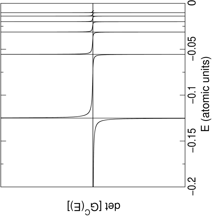
Figure 4.1: The determinant of a $3\times 3$ three-dimensional Coulomb Green’s matrix ${\rm det}[G^{C}(E)]$ as the function of the energy $E$ for $l=1$. The bound states of the Coulomb problem are located at energies where the vertical lines cross the horizontal axis. (These lines are shown only for demonstrative purposes, they do not correspond to the values of ${\rm det}[G^{C}(E)]$.) Atomic units of $m={\rm e}=\hbar=1$ and $Z=-1$ were used. For the sake of clarity only the first 6 energy levels are shown. These are located at $E_{n}=-1/[2(n+l+1)]^{2}$ with $n\leq 5$ according to (4.23).

4.3 Relativistic Coulomb Green’s operators

In this section we specify our method for relativistic Coulomb Green’s operators: the Coulomb Green’s operator of the Klein-Gordon and of the second order Dirac equations. The latter is physically equivalent to the conventional Dirac equation but seems to have several advantages from the mathematical point of view. For details see Ref. [58] and references therein.

The Hamiltonian of the radial Coulomb Klein–Gordon and second order Dirac equations are shown to possess an infinite symmetric tridiagonal matrix structure on the relativistic Coulomb–Sturmian basis. This allows us to give an analytic representation of the corresponding Coulomb Green’s operators in terms of continued fractions. The poles of the Green’s matrix reproduce the exact relativistic hydrogen spectrum.

It is noted here that the Coulomb–Sturmian matrix elements of the second order Dirac equation has already been obtained by Hostler [58] via evaluating complicated contour integrals. Our derivation, however is much simpler, it relies only on the Jacobi-matrix structure of the Hamiltonian, and the result obtained is also better suited for numerical calculations. In Hostler’s paper the results appear in terms of $\Gamma$ and hypergeometric functions, while our procedure results in an easily computable and analytically continuable continued fraction.

The radial Klein-Gordon and second order Dirac equation for Coulomb interaction are given by

$$H_{u}\left|\xi^{u}\right\rangle=0,$$ (4.38)

where

$$H_{u}=\left(\frac{E}{\hbar c}\right)^{2}-\mu^{2}+\frac{2\alpha Z}{\hbar c}\frac{E}{r}+\frac{d^{2}}{dr^{2}}-\frac{u\left(u+1\right)}{r^{2}}.$$ (4.39)

Here $\mu=mc/\hbar$, $\alpha=\mbox{e}^{2}/\hbar c$, $m$ is the mass and $Z$ denotes the charge. For the Klein-Gordon case $u$ is given by

$$u=-\frac{1}{2}+\sqrt{\frac{1}{4}+l(l+1)-(Z\alpha)^{2}},$$ (4.40)

and in the case of the second order Dirac equation for the different spin states we have

$$u_{\pm}=-\frac{1}{2}\mp\frac{1}{2}+\sqrt{\left(j+\frac{1}{2}\right)^{2}-(Z\alpha)^{2}}.$$ (4.41)

The relativistic Coulomb Green’s operator is defined as the inverse of the Hamiltonian $H_{u}$

$$H_{u}G_{u}=G_{u}H_{u}={\mathbf{1}}_{u},$$ (4.42)

where ${\mathbf{1}}_{u}$ denotes the unit operator of the radial Hilbert space ${\cal H}_{u}$.

In complete analogy with the non-relativistic case we can define the relativistic Coulomb–Sturmian functions as solutions of the Sturm-Liouville problem

$$\left(-\frac{d^{2}}{dr^{2}}+\eta^{2}+\frac{u\left(u+1\right)}{r^{2}}-\frac{2\eta(n+u+1)}{r}\right)S_{n;\eta}^{u}(r)=0,$$ (4.43)

where $\eta$ is a real parameter and $n=0,1,2,\ldots,\infty$ is the radial quantum number. They take the form

$$\left\langle r\left|nu;\eta\right.\right\rangle\equiv S_{n;\eta}^{u}(r)=\left[\frac{n!}{\left(n+2u+1\right)!}\right]^{\frac{1}{2}}\left(2\eta r\right)^{u+1}e^{-\eta r}L_{n}^{2u+1}(2\eta r),$$ (4.44)

where $L$ is a Laguerre-polinom. The relativistic Coulomb–Sturmian functions, together with their biorthonormal partner $\left\langle r\right.\widetilde{\left|nu;\eta\right\rangle}=1/r\cdot\left\langle r\right.\left|nu;\eta\right\rangle$, form a basis: i.e., they are orthogonal

$$\widetilde{\left\langle nu;\eta\right.}\left|mu;\eta\right\rangle=\left\langle nu;\eta\right.\widetilde{\left|mu;\eta\right\rangle}=\delta_{nm},$$ (4.45)

and form a complete set in ${\cal H}_{u}$

$$\sum_{n=0}^{\infty}{\left|nu;\eta\right\rangle}\widetilde{\left\langle nu;\eta\right|}=\sum_{n=0}^{\infty}\widetilde{\left|nu;\eta\right\rangle}\left\langle nu;\eta\right|={\mathbf{1}}_{u}.$$ (4.46)

A straightforward calculation yields

$$\begin{split}\left\langle nu;\eta\right|\!\left.mu;\eta\right\rangle\!\!&=\!\!\frac{1}{2\eta}\!\left[\!\delta_{nm}\!\left(2u+2n+2\right)-\delta_{nm-1\!}\sqrt{\left(n+1\right)\!\left(n+2u+2\right)}\right.\\ &\left.-\delta_{nm+1}\sqrt{n\left(2u+n+1\right)}\right].\end{split}$$ (4.47)

Utilizing this relation and considering Eq. (4.43) we can easily calculate the Coulomb–Sturmian matrix elements of $H_{u}$,

$$\begin{split}H_{nm}&:=\left\langle nu;\eta\right|H_{u}\left|mu;\eta\right\rangle=\\ &+\delta_{nm}\left(\frac{2\alpha zE}{\hbar c}-2(u+n+1)\eta+2(u+n+1)\frac{(E/\hbar c)^{2}-\mu^{2}+\eta^{2}}{2\eta}\right)\\ &-\delta_{nm-1}\left(\frac{(E/\hbar c)^{2}-\mu^{2}+\eta^{2}}{2\eta}\sqrt{(n+1)(n+2u+2)}\right)\\ &-\delta_{nm+1}\left(\frac{(E/\hbar c)^{2}-\mu^{2}+\eta^{2}}{2\eta}\sqrt{n(n+2u+1)}\right),\end{split}$$ (4.48)

which happen to possess a Jacobi-matrix structure.

Now the Coulomb–Sturmian matrix elements of the relativistic Coulomb Green’s operators

$$\left(G_{u}\right)_{nm}\equiv\widetilde{\left\langle nu;\eta\right|}G_{u}\widetilde{\left|mu;\eta\right\rangle}$$ (4.49)

corresponding to Hamiltonians (4.39), can be straightforwardly determined by using the continued fraction method of Equations (4.5) and (4.7) with the coefficients

$$u_{i}=-\frac{H_{ii-1}}{H_{ii+1}},\quad d_{i}=-\frac{H_{ii}}{H_{ii+1}}.$$ (4.50)

Again, the continued fraction representation convergent for bound-state energies and can be continued analytically to the whole complex energy plane.

4.3.1 Relativistic energy spectrum

In Table 4.3 we demonstrate the numerical precision of our Green’s matrix by evaluating the ground and some highly excited sates of relativistic hydrogen-like atoms, which, in fact, correspond to the poles of the Dirac Coulomb Green’s matrix. In particular, the poles of the determinant of (4.49) were located. Here we repeat again that irrespective of the rank $N$ of the Green’s matrix the poles should provide the exact Dirac results. In Table 4.3 we have taken $2\times 2$ matrices. Indeed, the results of this method, $E_{\text{cf}}$, agree with the exact one in all cases, practically up to machine accuracy, this way making possible the study of the fine structure splitting.

	energy levels	$E_{\mbox{cf}}$	$E_{\mbox{D}}$	$E_{\mbox{S}}$
hydrogen	$1$S1/2	$-0.5000066521$	$-0.5000066521$	$-0.5$
	$2$P1/2	$-0.1250020801$	$-0.1250020801$	$-0.125$
	$2$P3/2	$-0.1250004160$	$-0.1250004160$	$-0.125$
	$50$P1/2	$-0.0002000002$	$-0.0002000002$	$-0.0002$
	$50$P3/2	$-0.0002000001$	$-0.0002000001$	$-0.0002$
uranium	$1$S1/2	$-4861.1483347$	$-4861.1483347$	$-4232$
	$100$D3/2	$-0.4241695002$	$-0.4241695002$	$-0.4232$
	$100$D5/2	$-0.4238303306$	$-0.4238303306$	$-0.4232$

Table 4.3: Energy levels of hydrogen-like atoms in atomic units. $E_{\mbox{cf}}$ is the relativistic spectrum calculated via continued fraction, $E_{\mbox{ D }}$ and $E_{\mbox{\text{S}}}$ are textbook values of the relativistic Dirac and the non-relativistic Schrödinger spectrum, respectively.

4.4 D-dimensional harmonic oscillator

The Hamiltonian of the D-dimensional harmonic oscillator reveals a Jacobi matrix representation in the harmonic oscillator basis. Therefore the analytically calculated Jacobi-matrix elements can be utilized as the input of the continued fraction method for calculating harmonic oscillator basis representation of the Green’s operator corresponding to the harmonic oscillator potential.

The radial Hamiltonian describing the D-dimensional harmonic oscillator problem has the form

$$H^{HO}=\left[-\frac{\hbar^{2}}{2m}\left(\frac{\mbox{d}^{2}}{\mbox{d}r^{2}}-\frac{1}{r^{2}}\left(l+\frac{D-3}{2}\right)\left(l+\frac{D-1}{2}\right)\right)+\frac{1}{2}m\omega^{2}r^{2}\right],$$ (4.51)

where $\omega$ is the harmonic oscillator parameter. The energy eigenvalues are

$$E_{nl}=\hbar\omega\left(2n+l+\frac{D}{2}\right)$$ (4.52)

and the corresponding eigenfunctions can be written as

$$\langle r|\omega,nl\rangle=v^{\frac{1}{4}}\left(\frac{2\Gamma(n+1)}{\Gamma(n+l+\frac{D}{2})}\right)^{1/2}\exp(-\frac{v}{2}r^{2})(vr^{2})^{\frac{l}{2}+\frac{D-1}{4}}L_{n}^{(l+\frac{D}{2}-1)}(vr^{2}),$$ (4.53)

where $v=m\omega/\hbar$. The harmonic oscillator functions (4.53) with fixed $\omega$ are orthonormal and form a complete set in the usual sense

$$\langle\omega,n^{\prime}l|\omega,nl\rangle=\delta_{nn^{\prime}}$$ (4.54)

$${\bf 1}=\sum_{n=0}^{\infty}|\omega,nl\rangle\langle\omega,nl|.$$ (4.55)

The harmonic oscillator Hamiltonian (4.51) with parameter $\omega$ on the basis of the harmonic oscillator functions with different parameter $\omega^{\prime}$ takes a Jacobi-matrix form

$$\begin{split}\langle\omega^{\prime},nl|H^{HO}(\omega)&|\omega^{\prime},n^{\prime}l\rangle=\\ &+\delta_{nn^{\prime}}\left(\hbar\frac{\omega^{2}+{\omega^{\prime}}^{2}}{2\omega^{\prime}}\left(2n^{\prime}+l+\frac{D}{2}\right)\right)\\ &-\delta_{nn^{\prime}-1}\hbar\frac{\omega^{2}-{\omega^{\prime}}^{2}}{2\omega^{\prime}}\left(n^{\prime}\left(n^{\prime}+l+\frac{D}{2}-1\right)\right)^{1/2}\\ &-\delta_{nn^{\prime}+1}\hbar\frac{\omega^{2}-{\omega^{\prime}}^{2}}{2\omega^{\prime}}\left((n^{\prime}+1)\left(n^{\prime}+l+\frac{D}{2}\right)\right)^{1/2}\end{split}$$ (4.56)

The general method of Section 4.1 requires the knowledge of the matrix elements $J_{ij}=\langle\omega^{\prime},il|E-H^{HO}(\omega)|\omega^{\prime},jl\rangle$ which readily follows from (4.54) and (4.56) according to

$$J_{ij}=E\times\delta_{ij}-\langle\omega^{\prime},il|H^{HO}(\omega)|\omega^{\prime},jl\rangle.$$ (4.57)

The calculation of the Green’s matrix $G_{ij}(E)=\langle\omega^{\prime},il|G(E,\omega)|\omega^{\prime},jl\rangle$ goes similarly to the previous sections making use of formulae (4.5) and (4.7).

It is impossible to overestimate the importance of the harmonic oscillator in theoretical physics. Here I would like only to mention one exotic topic, the physics of anyons, which are quantum mechanically indistinguishable particles following fractional statistics, where the harmonic oscillator potential plays an important role [59].

4.5 The generalized Coulomb potential

Quantum mechanical models and practical calculations often rely on some exactly solvable models like the Coulomb and the harmonic oscillator potentials. The actual example we consider here is the generalized Coulomb potential introduced by Lévai and Williams [60], which is the member of the Natanzon confluent potential class [61]. This potential is Coulomb-like asymptotically, while its short-range behavior depends on the parameters: it can be finite or singular as well at the origin. Its shape therefore can approximate various realistic problems, such as nuclear potentials with relatively flat central part, or atomic potentials that incorporate the effect of inner closed shells by a phenomenological repulsive core. Another interesting feature of the D-dimensional generalized Coulomb potential is that it contains the Coulomb and harmonic oscillator potentials as limiting cases, this way providing a smooth transition between the Coulomb and the harmonic oscillator problems in various dimensions.

More and more interactions can be modelled by making advantage of the rather flexible potential shapes offered by exactly solvable potentials. Virtually all quantum mechanical methods rely in some respect on analytically solvable potentials. Very often their wave function solutions are used as Hilbert space bases. More powerful methods can be constructed if we select a basis which allows the exact analytical calculation of the Green’s operator of an analytically solvable potential.

In this section we show that an appropriate Sturm–Liuville basis can be defined on which the matrix elements of the Hamiltonian exhibit a Jacobi matrix. The corresponding Green’s matrix then follows from the method of Section 4.1.

4.5.1 The potential

Let us consider the radial Schrödinger equation in D spatial dimensions with a potential $V(r)$ that depends only on the radial variable $r$

$$H\psi(r)\equiv\left(-\frac{{\rm d}^{2}}{{\rm d}r^{2}}+\frac{1}{r^{2}}(l+\frac{D-3}{2})(l+\frac{D-1}{2})+v(r)\right)\psi(r)=\epsilon\psi(r)\ ,$$ (4.58)

where $v(r)\equiv 2m\hbar^{-2}V(r)$ and $\epsilon\equiv 2m\hbar^{-2}E$. We define the generalized Coulomb potential [60] in D-dimension as

$$\begin{split}v(r)=&-\frac{1}{r^{2}}(l+\frac{D-3}{2})(l+\frac{D-1}{2})+(\beta-\frac{1}{2})(\beta-\frac{3}{2})\frac{C}{4h(r)(h(r)+\theta)}\\ &-\frac{q}{h(r)+\theta}-\frac{3C}{16(h(r)+\theta)^{2}}+\frac{5C\theta}{16(h(r)+\theta)^{3}}\ ,\end{split}$$ (4.59)

where $h(r)$ is defined in terms of its inverse function

$$r=r(h)=C^{-\frac{1}{2}}\left[\theta\tanh^{-1}\left(\left(\frac{h}{h+\theta}\right)^{\frac{1}{2}}\right)+(h(h+\theta))^{\frac{1}{2}}\right]\ .$$ (4.60)

The $h(r)$ function maps the $[0,\infty)$ half axis onto itself and can be approximated with $h(r)\simeq C^{\frac{1}{2}}r$ and $h(r)\simeq Cr^{2}/(4\theta)$ in the $r\rightarrow\infty$ and $r\rightarrow 0$ limits, respectively.

Bound states are located at

$$\epsilon_{n}=-\frac{C}{4}\rho_{n}^{2}\ ,$$ (4.61)

where

$$\rho_{n}=\frac{2}{\theta}\left[\left((n+\beta/2)^{2}+\frac{q\theta}{C}\right)^{\frac{1}{2}}-(n+\beta/2)\right]\ ,$$ (4.62)

and the bound-state wave functions can be written in terms of associated Laguerre–polynomials as

$$\begin{split}\psi_{n}(r)&=C^{\frac{1}{4}}\rho_{n}^{\frac{\beta+1}{2}}\left(\frac{\Gamma(n+1)}{\Gamma(n+\beta)(2n+\beta+\rho_{n}\theta)}\right)^{1/2}\\ &\times(h(r)+\theta)^{\frac{1}{4}}(h(r))^{\frac{2\beta-1}{4}}\exp(-\frac{\rho_{n}}{2}h(r))L_{n}^{(\beta-1)}(\rho_{n}h(r))\ .\end{split}$$ (4.63)

Potential (4.59) clearly carries angular momentum dependence: its first term merely compensates the centrifugal term arising from the kinetic term of the Hamiltonian. Its second term also has $r^{-2}$-like singularity (due to $h^{-1}(r)$) and it cancels the angular momentum dependent term in the two important limiting cases that recover the $D$-dimensional Coulomb and the harmonic oscillator potentials. The third term of (4.59) represents an asymptotically Coulomb–like interaction, while the remaining two terms behave like $r^{-2}$ and $r^{-3}$ for large values of $r$. The long-range behavior of potential (4.59) suggests its use in problems associated with the electrostatic field of some charge distribution. The deviation from the Coulomb potential close to the origin can be viewed as if the point-like charge could be replaced with an extended charged object. The relevant charge density is readily obtained from the potential using

$$\rho(r)=-\frac{\hbar^{2}}{8\pi m{\rm e}}\Delta v(r)\ .$$ (4.64)

In Figures 4.2 and 4.3 we present examples for the actual shape of potential (4.59) and the corresponding charge distribution (4.64) for various values of the parameters. It can be seen that this potential is suitable for describing the Coulomb field of extended objects. It is a general feature of potential (4.59) that for small values of $\theta$ a (finite) positive peak appears near the origin, which also manifests itself in a repulsive “soft core”, corresponding to a region with positive charge density (see Fig. 4.3).

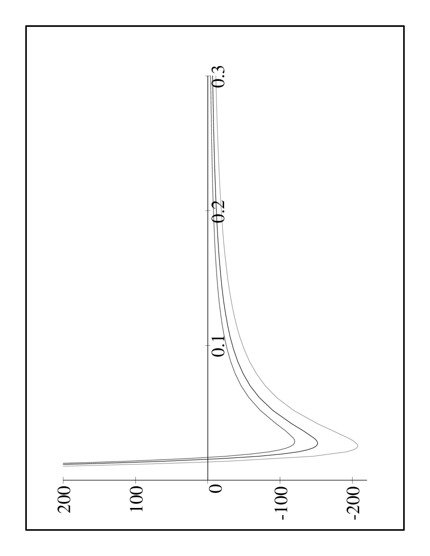
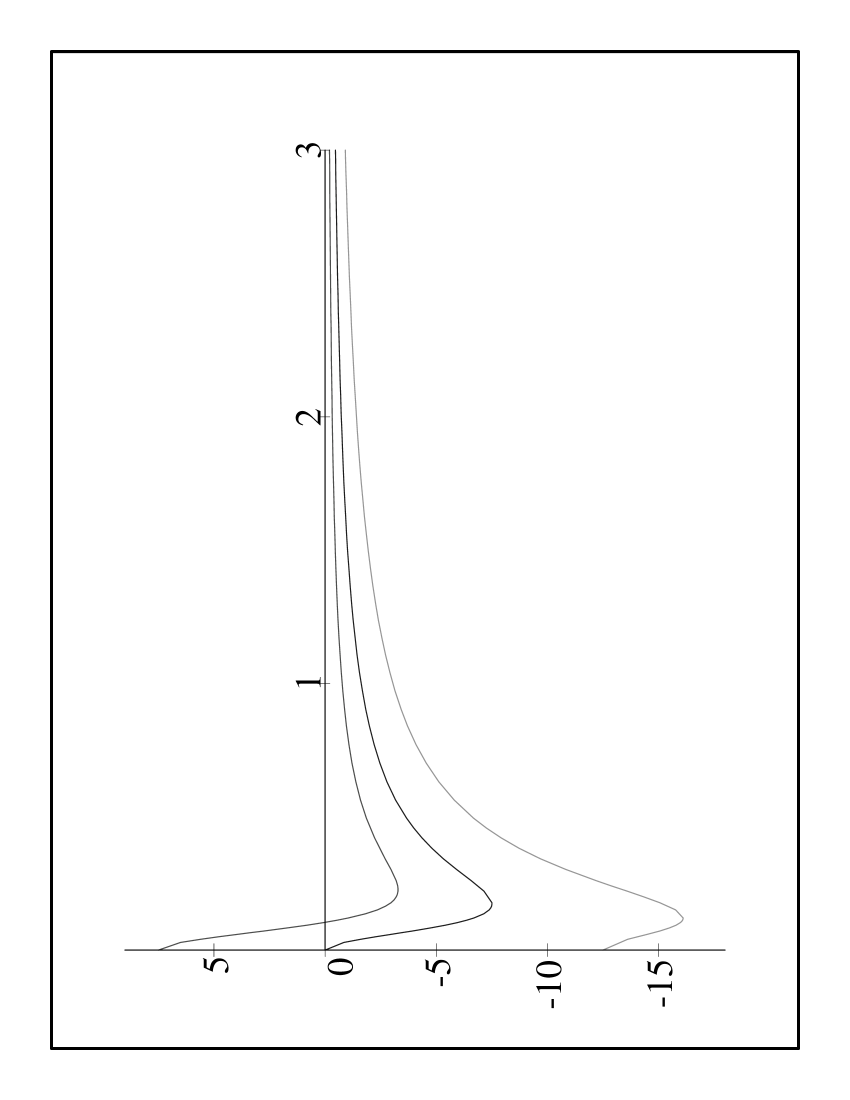
$\theta=0.01$	$\theta=0.1$	$\theta=1$

Figure 4.2: The generalized Coulomb potential for $q$=0.5, 1.25, 2.5; $\theta$=0.01, 0.1, 1; $C$=1 and $\beta=3/2$. $l=0$ and $D=3$ is also implied. In each panel the largest $q$ corresponds to the lowest curve. Note the different scales of the horizontal ($r$) and the vertical ($v(r)$) axes.

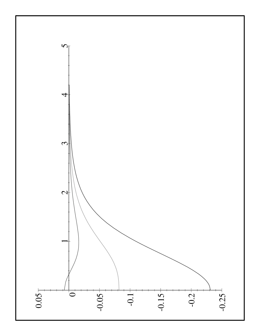
Figure 4.3: The charge distributions corresponding to the potentials displayed in Fig. 4.2 for $\theta$=1 and $q$=0.5, 1.25, 2.5. (The largest $q$ corresponds to the lowest curve.)

The Coulomb and harmonic oscillator limits

The special limits of the generalized Coulomb potential can be realized by specific choices of the parameters in Eq. (4.60):

The $D$-dimensional Coulomb limit follows from the $\theta\rightarrow 0$ limit and it is recovered from Eq. (4.59) by the $\beta=2l+D-1$ and $C^{-\frac{1}{2}}q=2mZ{\rm e}^{2}/\hbar^{2}$, choices: the third term of (4.59) becomes the Coulomb term, the fifth one vanishes, while the other three terms becoming proportional with $r^{-2}$ cancel out completely.

In order to reach the oscillator limit one has to take $\theta\rightarrow\infty$ keeping $C/\theta\equiv\tilde{C}$ constant together with the redefinition of the potential (4.59) and the energy eigenvalues by adding $q/\theta$ to both. This choice simply represents resetting the energy scale: $\epsilon=0$ corresponds to $v(r\rightarrow\infty)$ for the Coulomb problem, and to $v(r=0)$ for the harmonic oscillator. (Note that the energy eigenvalues also have different signs in the two cases.) Besides $C/\theta=\tilde{C}$, the $\tilde{q}\equiv q/\theta^{2}$ parameter also has to remain constant in the $\theta\rightarrow\infty$ transition here. The potential thus adapted to the harmonic oscillator limit reads

$$\begin{split}\tilde{v}(r)&\equiv v(r)+q\theta=\\ &\quad-\frac{1}{r^{2}}\left(l+\frac{D-3}{2}\right)\left(l+\frac{D-1}{2}\right)+\left(\beta-\frac{1}{2}\right)\left(\beta-\frac{3}{2}\right)\frac{\tilde{C}}{4h(r)(1+\frac{h(r)}{\theta})}\\ &\quad-\frac{\tilde{q}h(r)}{1+\frac{h(r)}{\theta}}-\frac{3\tilde{C}}{16\theta}\frac{1}{\left(1+\frac{h(r)}{\theta}\right)^{2}}+\frac{5\tilde{C}}{16\theta}\frac{1}{\left(1+\frac{h(r)}{\theta}\right)^{3}}\ .\end{split}$$ (4.65)

The harmonic oscillator potential is recovered from (4.65) by the $\beta=l+D/2$ and $\tilde{C}\tilde{q}=(2m\omega/\hbar)^{2}$ choice. The two last terms in (4.65) vanish, the first and the second cancel out, while the third one reproduces the harmonic oscillator potential. The new form of the energy eigenvalues is

$$\tilde{\epsilon}_{n}\equiv\epsilon_{n}+q/\theta=\tilde{C}(2n+\beta)\left[\left(\frac{1}{\theta^{2}}(n+\frac{\beta}{2})^{2}+\frac{\tilde{q}}{\tilde{C}}\right)^{\frac{1}{2}}-\frac{1}{\theta}(n+\frac{\beta}{2})\right],$$ (4.66)

which indeed, reduces to the $\tilde{\epsilon}_{n}=(2m\omega/\hbar)(2n+l+D/2)$ oscillator spectrum in the $\theta\rightarrow\infty$ limit. The wave functions (4.63) are unchanged, except for the redefinition of the parameters.

4.5.2 The matrix elements of the Green’s operator

We define the generalized Coulomb–Sturmian basis as the solution of the generalized Sturm–Liouville equation. The Sturm–Liouville equation, which depends on $n$ as a parameter and corresponds to the generalized Coulomb potential (4.59), reads

$$\Bigg{[}-\frac{{\rm d}^{2}}{{\rm d}r^{2}}-\frac{3C}{16(h(r)+\theta)^{2}}+\frac{5C\theta}{16(h(r)+\theta)^{3}}+\frac{C(\beta-\frac{1}{2})(\beta-\frac{3}{2})}{4h(r)(h(r)+\theta)}\\ -\left(\frac{\rho^{2}\theta}{4}+\rho(n+\frac{\beta}{2})\right)\frac{C}{h(r)+\theta}+\frac{C}{4}\rho^{2}\Bigg{]}\phi(\rho,r)=0\ ,$$ (4.67)

and is solved by the generalized Coulomb–Sturmian (GCS) functions

$$\langle r|n\rangle\equiv\phi_{n}(\rho,r)=\\ \left(\frac{\Gamma(n+1)}{\Gamma(n+\beta)}\right)^{1/2}(\rho h(r)+\rho\theta)^{\frac{1}{4}}(\rho h(r))^{\frac{2\beta-1}{4}}\exp(-\frac{\rho}{2}h(r))L_{n}^{(\beta-1)}(\rho h(r))\ .$$ (4.68)

Here $\rho$ is a parameter characterizing the generalized Coulomb–Sturmian basis. The GCS functions, being solutions of a Sturm–Liouville problem, have the property of being orthonormal with respect to the weight function $C^{\frac{1}{2}}(h(r)+\theta)^{-1}$. Introducing the notation $\langle r|\widetilde{n}\rangle\equiv\phi_{n}(\rho,r)C^{\frac{1}{2}}(h(r)+\theta)^{-1}$ the orthogonality and completeness relation of the GCS functions can be expressed as

$$\begin{split}\langle n^{\prime}|\widetilde{n}\rangle&=\delta_{n^{\prime}n}\\ {\bf 1}=\sum_{n=0}^{\infty}|\widetilde{n}\rangle\langle n|&=\sum_{n=0}^{\infty}|n\rangle\langle\widetilde{n}|\ .\end{split}$$ (4.69)

Analytic calculations yield that both the overlap of two GCS functions and the $H_{n^{\prime}n}=\langle n^{\prime}|H|n\rangle$ Hamiltonian matrix possesses a tridiagonal form, therefore the matrix elements of the $\epsilon-H$ operator also have this feature

$$\begin{split}\langle n|\epsilon-H|n^{\prime}\rangle=&+\delta_{nn^{\prime}}\left[\frac{\epsilon}{C^{\frac{1}{2}}\rho}(2n+\beta-\rho\theta)-\frac{C^{\frac{1}{2}}\rho}{4}\left(-\frac{4q}{C\rho}+(2n+\beta)\right)\right]\\ &-\delta_{nn^{\prime}+1}\left(n(n+\beta-1)\right)^{\frac{1}{2}}\left(\frac{\epsilon}{C^{\frac{1}{2}}\rho}+\frac{C^{\frac{1}{2}}\rho}{4}\right)\\ &-\delta_{nn^{\prime}-1}\left((n+1)(n+\beta)\right)^{\frac{1}{2}}\left(\frac{\epsilon}{C^{\frac{1}{2}}\rho}+\frac{C^{\frac{1}{2}}\rho}{4}\right)\ .\end{split}$$ (4.70)

This means, that similarly to the previous sections the matrix elements of the Green’s operator in the GCS basis, $G_{ij}=\langle\widetilde{n}|G|\widetilde{n}\rangle$, can be determined by using continued fractions, as described in Section 4.1 utilizing the analytically known Jacobi-matrix elements of (4.70).

Chapter 5 Applications

The continued fraction method for calculating Green’s matrices on the whole complex energy plane together with methods for solving integral equations in discrete Hilbert space basis representation provide a rather general and easy-to-apply quantum mechanical approximation scheme.

In the first part of this chapter the continued fraction representation of the Coulomb–Sturmian space Coulomb Green’s operator (Section 4.2) is used for solving the two-body Lippmann–Schwinger equation with a potential modelling the interaction of two $\alpha$ particles in order to find bound, resonance and scattering solutions.

In the second part of this chapter our Green’s operator is applied for solving the Coulomb three-body bound state problem in the Faddeev–Merkuriev integral equation approach. In particular, the binding energy of the Helium atom is determined by solving the Faddeev–Merkuriev equations in the Coulomb–Sturmian space representation.

Both solution schemes have been devised by Papp in Refs. [25, 27, 28, 29] and Refs. [16, 30], respectively. We demonstrate here that the continued fraction representation of the Coulomb Green’s operator in practice is as good as the original one given by Papp in terms of hypergeometric functions.

The two examples of this chapter are intended to show the importance of the analytic representation of the Green’s operators through the efficiency of the discrete Hilbert space expansion method for solving fundamental integral equations.

5.1 Model nuclear potential calculation

In this section we apply the method of Refs. [25, 27, 28, 29] together with the continued fraction representation of the Coulomb Green’s operator in order to calculate bound, resonant and scattering state solutions of a potential problem in a unified manner. The particular example we consider here is a potential modelling the interaction of two $\alpha$ particles. This example is thoroughly discussed in the pedagogical work [62] in the context of a conventional approach based on the numerical solution of the Schrödinger equation.

The interaction of two $\alpha$ particles can be approximated by the potential

$${V}_{\alpha-\alpha}(r)=-A\exp(-\beta r^{2})+\frac{Z^{2}{\rm e}^{2}}{r}\ {\rm erf}(\gamma r),$$ (5.1)

where ${\rm erf}(z)$ is the error function [56]. This potential is a composition of a bell-shaped deep, attractive nuclear potential, and a repulsive electrostatic field between two extended charged objects. The units used in the Hamiltonian of this system are suited to nuclear physical applications, i.e. the energy and length scale are measured in MeV and fm, respectively. In these units $\hbar/(2m)=10.375$ MeV fm² ($m$ is the reduced mass of two $\alpha$ particles) and ${\rm e}^{2}=1.44$ MeV fm. The other parameters are $A=$122.694 MeV, $\beta=0.22$ fm^-2, $\gamma=0.75$ fm^-1 and $Z=2$ (the charge number of the $\alpha$ particles).

Our radial Hamiltonian $H_{l}$ containing the model potential (5.1) can be split into two terms

$$H_{l}=H_{l}^{\rm C}+V_{l}\ .$$ (5.2)

Here $V_{l}$ is the asymptotically irrelevant short-range potential and $H_{l}^{\rm C}$ denotes the asymptotically relevant radial Coulomb Hamiltonian (4.22). Since the $\alpha-\alpha$ potential possesses a Coulomb tail, the short-range potential is defined by

$$V_{l}(r)=V_{\alpha-\alpha}(r)-\frac{Z^{2}{\rm e}^{2}}{r}=-A\exp(-\beta r^{2})-\frac{Z^{2}{\rm e}^{2}}{r}\ {\rm erfc}(\gamma r),$$ (5.3)

with ${\rm erfc}(z)=1-{\rm erf}(z)$.

The bound, resonant and scattering state solutions of the potential problem characterized by the Hamiltonian $H_{l}$ can be obtained by solving the Lippmann–Schwinger integral equation. The bound and resonant state wave functions satisfy the homogeneous Lippmann–Schwinger equation

$$|\Psi_{l}\rangle=G_{l}^{\rm C}(E)V_{l}|\Psi_{l}\rangle$$ (5.4)

at real negative and complex $E$ energies, respectively. While the wave function $|\Psi^{(\pm)}_{l}\rangle$ describing a scattering process satisfies the inhomogeneous Lippmann–Schwinger equation (Section 2.3)

$$|\Psi^{(\pm)}_{l}\rangle=|\Phi^{(\pm)}_{l}\rangle+G_{l}^{\rm C}(E\pm{\rm i}0)V_{l}|\Psi^{(\pm)}_{l}\rangle\ ,$$ (5.5)

where $|\Phi^{(\pm)}_{l}\rangle$ is the solution to the Hamiltonian $H^{\rm C}_{l}$ with scattering asymptotics. In Equations (5.4), (5.5) $G^{\rm C}_{l}(z)$ denotes the radial Coulomb Green’s operator defined as $G^{\rm C}_{l}(z)=(z-H^{\rm C}_{l})^{-1}$.

We are going to solve these equations by using a discrete Hilbert space basis representation in a unified way by approximating only the potential term $V_{l}$. For this purpose we write the unit operator in the form

$${\bf 1}=\lim_{N\to\infty}{\bf{1}}_{N}\ ,$$ (5.6)

where

$${\bf{1}}_{N}=\sum_{n=0}^{N}|\tilde{n}\rangle\sigma_{n}^{N}\langle n|=\sum_{n=0}^{N}|n\rangle\sigma_{n}^{N}\langle\tilde{n}|\ .$$ (5.7)

In this case the $\{|n\rangle,|\tilde{n}\rangle\}$ biorthonormal basis is specified as the Coulomb–Sturmian basis (4.25). The $\sigma$ factors have the properties $\lim_{n\to\infty}\sigma_{n}^{N}=0$ and $\lim_{N\to\infty}\sigma_{n}^{N}=1$, and render the limiting procedure in (5.6) smoother. They were introduced originally for improving the convergence properties of truncated trigonometric series [63], but they turned out to be also very efficient in solving integral equations in discrete Hilbert space basis representation [64]. The choice of $\sigma_{n}^{N}$

$$\sigma_{n}^{N}=\frac{1-\exp\{-[\alpha(n-N-1)/(N+1)]^{2}\}}{1-\exp(-\alpha^{2})}$$ (5.8)

with $\alpha\sim 5$ has proved to be appropriate in practical calculations.

Let us introduce an approximation of the potential operator

$$V_{l}={\bf 1}V_{l}{\bf 1}\approx{\bf{1}}_{N}V_{l}{\bf{1}}_{N}=V_{l}^{N}=\sum_{n,n^{\prime}=0}^{N}|\widetilde{n}\rangle\;\underline{V}_{nn^{\prime}}\;\mbox{}\langle\widetilde{n^{\prime}}|\ ,$$ (5.9)

where the matrix elements

$$\underline{V}_{nn^{\prime}}=\sigma^{N}_{n}\langle n|V_{l}|n^{\prime}\rangle\sigma^{N}_{n^{\prime}}\ ,$$ (5.10)

in general, are to be calculated numerically. This approximation is called separable expansion, because the operator $V_{l}^{N}$, e.g. in coordinate representation, takes the form

$$\langle r|V^{N}|r^{\prime}\rangle=\sum_{n,n^{\prime}=0}^{N}\langle r|\widetilde{n}\rangle\;\underline{V}_{nn^{\prime}}\;\mbox{}\langle\widetilde{n^{\prime}}|r^{\prime}\rangle\ ,$$ (5.11)

i.e.  the dependence on $r$ and $r^{\prime}$ appears in a separated functional form.

With this separable potential Eqs. (5.4) and (5.5) are reduced to

$$|\Psi_{l}\rangle=\sum_{n,n^{\prime}=0}^{N}G_{l}^{\rm C}(E)|\widetilde{n}\rangle\;\underline{V}_{nn^{\prime}}\;\mbox{}\langle\widetilde{n^{\prime}}|\Psi_{l}\rangle\$$ (5.12)

and

$$|\Psi^{(\pm)}_{l}\rangle=|\Phi^{(\pm)}_{l}\rangle+\sum_{n,n^{\prime}=0}^{N}G^{\rm C}_{l}(E\pm{\rm i}0)|\widetilde{n}\rangle\;\underline{V}_{nn^{\prime}}\;\mbox{}\langle\widetilde{n^{\prime}}|\Psi^{(\pm)}_{l}\rangle\ ,$$ (5.13)

respectively. To derive equations for the coefficients $\underline{\Psi}_{l}^{(\pm)}=\langle\widetilde{n^{\prime}}|\Psi_{l}^{(\pm)}\rangle$ and $\underline{\Psi}_{l}=\langle\widetilde{n^{\prime}}|\Psi_{l}\rangle$, we have to act with states $\langle\widetilde{n^{\prime\prime}}|$ from the left. Then the following homogeneous and inhomogeneous algebraic equations are obtained, for bound and scattering state problems, respectively:

$$[(\underline{G}_{l}^{\rm C}(E))^{-1}-\underline{V}_{l}]\underline{\Psi}_{l}=0$$ (5.14)

and

$$[(\underline{G}^{\rm C}_{l}(E\pm{\rm i}0))^{-1}-\underline{V}_{l}]\underline{\Psi}_{l}^{(\pm)}=\underline{\Phi}_{l}^{(\pm)},$$ (5.15)

where the overlap ${\Phi}_{nl}^{(\pm)}=\langle\widetilde{n}|\Phi_{l}^{(\pm)}\rangle$ can also be calculated analytically [27]. The homogeneous equation (5.14) is solvable if and only if

$$\det[(\underline{G}_{l}^{\rm C}(E))^{-1}-\underline{V}_{l}]=0$$ (5.16)

holds, which is an implicit nonlinear equation for the bound and resonant state energies. As far as the scattering states are concerned the solution of (5.15) provides the overlap $\langle\widetilde{n}|\Psi_{l}\rangle$. From this quantity any scattering information can be inferred, for example the scattering amplitude corresponding to potential $V_{l}$ is given by [19]

$$A^{V}=\langle\Phi^{(-)}_{l}|V_{l}|\Psi^{(+)}_{l}\rangle=\underline{\Phi}_{l}^{(-)}\underline{V}_{l}\;\underline{\Psi}_{l}^{(+)}.$$ (5.17)

Note that also the Green’s matrix of the total Hamiltonian, which is equivalent with the complete solution to the physical system, can be constructed as

$$\underline{G}_{l}(z)=[(\underline{G}_{l}^{\rm C}(z))^{-1}-\underline{V}_{l}]^{-1}\ .$$ (5.18)

Finally, it should also be emphasized, that in this approach only the potential operator is approximated, but the asymptotically important $H^{\rm C}$ term remains intact. The properties of the short-range potential is buried into the numerical values of the matrix elements. Thus the method is applicable to all types of potentials, as long as we can calculate their matrix elements somehow. Beside usual potentials this equally applies to complex, momentum-dependent, non-local, etc.  potentials relevant to practical problems of atomic, nuclear and particle physics. Furthermore, the present formalism is equally suited to problems including attractive or repulsive long-range Coulomb-like and short-range potentials. The solutions are defined on the whole Hilbert space, not only on a finite subspace. The wave functions are not linear combinations of the basis functions, but rather, as Eqs. (5.13) and (5.12) indicate, linear combinations of the states $G_{l}^{\rm C}(E)|\widetilde{n}\rangle$, which have been shown to possess correct Coulomb asymptotics [28].

5.1.1 Bound states

First we consider only the nuclear part of potential (5.1) and switch off the Coulomb interaction by setting $Z=0$. According to Ref. [62], this potential supports altogether four bound states: three with $l=0$ and one with $l=2$. However, it is known that the first two $l=0$ and the single $l=2$ state are unphysical, since they are forbidden because of the Pauli principle. This fact is not taken into account in this simple potential model. Although from the physical point of view these Pauli-forbidden states have to be dismissed as unphysical, they are legitimate solutions to our simple model potential. The proper inclusion of the Pauli principle into the model would turn the potential into a non-local one. This problem has been considered within the present method in Ref. [27].

In Table 5.1 we present the results of our calculations for the three $l=0$ states showing the convergence of the method with respect to $N$, the number of basis states used in the expansion. We determined the energies of these states from Eq. (5.16), using the CS parameter $b=4$ fm^-1. It can be seen that the method is very accurate, convergence up to 12 digits can easily been reached. We note that according to Ref. [62], the energy of the two lowest (i.e. the unphysical) $l=0$ states is $E=-76.903\ 6145$ and $E=-29.000\ 48$ MeV in the uncharged case, which is in reasonable agreement with our results.

$N$	$E_{00}$ (MeV)	$E_{10}$ (MeV)	$E_{20}$ (MeV)
8	$-$76.903 557 1529	$-$29.005 234 9134	$-$1.739 478 2626
10	$-$76.903 609 9717	$-$29.000 352 3141	$-$1.637 269 0831
15	$-$76.903 614 3090	$-$29.000 469 8249	$-$1.608 824 6403
18	$-$76.903 614 3254	$-$29.000 470 2338	$-$1.608 742 5166
20	$-$76.903 614 3263	$-$29.000 470 2566	$-$1.608 741 0685
25	$-$76.903 614 3265	$-$29.000 470 2623	$-$1.608 740 8256
28	$-$76.903 614 3265	$-$29.000 470 2625	$-$1.608 740 8216
30	$-$76.903 614 3265	$-$29.000 470 2625	$-$1.608 740 8213
35	$-$76.903 614 3265	$-$29.000 470 2626	$-$1.608 740 8214
40	$-$76.903 614 3265	$-$29.000 470 2626	$-$1.608 740 8214

Table 5.1: Convergence of the $l=0$ bound state energy eigenvalues $E_{nl}$ in $V_{\alpha-\alpha}(r)$ in the uncharged ($Z=0$) case. $N$ denotes the number of basis states used in the expansion.

5.1.2 Resonance states

Switching on the repulsive Coulomb interaction ($Z=2$) the bound states are shifted to higher energies. The most spectacular effect is that the third $l=0$ state, which is located at $E=-1.608\ 740\ 8214$ MeV in the uncharged case, moves to positive energies and becomes a resonant state. This is in agreement with the observations: the $\alpha-\alpha$ system (i.e. the ⁸Be nucleus) does not have a stable ground state, rather it decays with a half life of $7\times 10^{-17}$ sec.

In our calculations we determined the energies corresponding to this resonance and to other ones as well by the same techniques we used before to find bound states. In fact, we used the same computer code and the same CS parameter ($b=4$ fm^-1) as we used in the analysis of bound states. The method, again, requires locating the poles of the Green’s matrix, but not on the real energy axis, rather on the complex energy plane.

In Table 5.2 we demonstrate the convergence of our method with respect to $N$ for the lowest $l=0$ and $l=2$ resonance states. In Fig. 5.1 we plotted the modulus of the determinant of the (5.18) Green’s matrix over the complex energy plane for $l=2$. The resonance is located at the pole of this function. Finally, we mention that there is a resonance state for $l=4$ at $E_{{\rm res},4}=11.791\ 038-{\rm i\ }1.788\ 957$ MeV.

Although it is not our aim here to reproduce experimental data with this simple potential model, we note that the corresponding experimental values [65] are $E_{{\rm res},l=0}=$0.09189 MeV, $E_{{\rm res},l=2}=$3.132 $\pm$ $0.030$ MeV, $E_{{\rm res},l=4}=$11.5 $\pm$ 0.3 MeV, and $\Gamma_{l=0}/2=(3.4\pm 0.9)\times 10^{-6}$ MeV, $\Gamma_{l=2}/2$=0.750 $\pm$ 0.010 MeV, $\Gamma_{l=4}/2\simeq$1.75 MeV.

$N$	$E_{{\rm res},0}$ (MeV)	$E_{{\rm res},2}$ (MeV)
8	$-$0.000 854 9596 $+$i 0.000 000 0000	2.807 21 $-$i 0.607 11
10	$-$0.063 364 2503 $-$i 0.000 000 0681	2.866 30 $-$i 0.628 56
15	$-$0.091 785 0787 $-$i 0.000 002 8092	2.889 68 $-$i 0.620 99
18	$-$0.091 963 0277 $-$i 0.000 002 8572	2.889 34 $-$i 0.620 53
20	$-$0.091 969 7296 $-$i 0.000 002 8588	2.889 24 $-$i 0.620 56
25	$-$0.091 971 8479 $-$i 0.000 002 8592	2.889 23 $-$i 0.620 62
28	$-$0.091 971 9788 $-$i 0.000 002 8592	2.889 25 $-$i 0.620 62
30	$-$0.091 972 0064 $-$i 0.000 002 8592	2.889 25 $-$i 0.620 61
35	$-$0.091 972 0258 $-$i 0.000 002 8592	2.889 24 $-$i 0.620 61
40	$-$0.091 972 0290 $-$i 0.000 002 8592	2.889 25 $-$i 0.620 61

Table 5.2: Convergence of the energy eigenvalues $E_{{\rm res},l}$ for the $l=0$ and $l=2$ resonances in the $V_{\alpha-\alpha}(r)$ potential. $N$ denotes the number of basis states used in the expansion.

Figure 5.1: The modulus of the determinant of the $\underline{G}(E)$ Green’s matrix for the $\alpha-\alpha$ potential on the complex energy plane for $l=2$. The pole at $E=2.889\ 25-{\rm i\ }0.620\ 61$ MeV corresponds to a resonance.

5.1.3 Scattering states

In order to demonstrate the performance of our approach for scattering states we calculated scattering phase shifts $\delta_{l}(E)$ for ${V}_{\alpha-\alpha}(r)$ in (5.1). As described previously in this subsection, phase shifts can be extracted from the scattering amplitude given in Eq. (5.17). Specifying this formula for the Coulomb–like case and for a given partial wave $l$ we have

$$a_{l}=\frac{1}{k}\exp({\rm i}(2\eta_{l}+\delta_{l}))\sin\delta_{l}\ ,$$ (5.19)

where $a_{l}$ is the Coulomb–modified scattering amplitude corresponding to the short-range potential, $\eta_{l}={\rm arg}\Gamma(l+i\gamma+1))$ is the phase shift of the Coulomb scattering with $\gamma=Z^{2}{\rm e}^{2}m/\hbar^{2}k$ and $\delta_{l}$ is the phase shift due to the short-range potential.

The convergence of the phase shifts with respect to $N$ is demonstrated in Table 5.3, where $\delta_{0}(E)$ is displayed at three different energy values. As in our calculations for the bound and the resonance states, we used $b=4$ fm^-1here too.

In Fig. 5.2 we plotted the scattering phase shifts $\delta_{l}(E)$ for $l=0$, 2 and 4 up to $E=30$ MeV. In all three plots in Fig. 5.2 the location of the corresponding resonance is clearly visible as a sharp rise of the phase around the resonance energy $E_{\rm res}$. This rise is expected to be more sudden for sharp resonances, and this is, in fact, the case here too. The phase changes with an abrupt jump of $\pi$ for the sharp $l=0$ resonance, while it is slower for the broader $l=2$ and $l=4$ resonances. We also note that the phase shifts plotted in Fig. 5.2 are also in accordance with the Levinson theorem, which states that $\delta_{l}(0)=m\pi$, where $m$ is the number of bound states in the particular angular momentum channel. Indeed, as we have discussed earlier, there are two bound states for $l=0$, one for $l=2$ and none for $l=4$.

As an illustration of the importance of the smoothing factors we show in Fig. 5.3 the convergence of the phase shift $\delta_{0}(E)$ at a specific energy $E=10$ MeV with and without the smoothing factors $\sigma_{n}^{N}$ in (5.7), and consequently in (5.10). (Here and everywhere else the $\alpha$ parameter of the (5.8) $\sigma$ factors was chosen to be 5.2.) Clearly, the convergence is much poorer without the smoothing factors. We note that this also applies to other quantities calculated for bound and resonance states.

$N$	$E=0.1$ MeV	$E=1$ MeV	$E=30$ MeV
8	6.283 230	8.817 731	7.783 217
10	9.424 059	8.862 581	4.817 163
15	9.424 018	8.859 651	4.835 479
18	9.424 022	8.859 467	4.829 861
20	9.424 023	8.859 441	4.828 882
25	9.424 024	8.859 419	4.828 563
28	9.424 024	8.859 414	4.828 555
30	9.424 024	8.859 412	4.828 554
35	9.424 024	8.859 411	4.828 552
40	9.424 024	8.859 411	4.828 552

Table 5.3: Convergence of the $\delta_{0}(E)$ phase shift (in radians) in the $V_{\alpha-\alpha}(r)$ potential at three different energies. $N$ denotes the number of basis states used in the expansion.

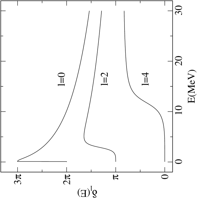
Figure 5.2: Scattering phase shifts $\delta_{l}(E)$ (in radians) in the $\alpha-\alpha$ potential for $l=0$, 2 and 4. The resonances in these partial waves appear as sharp rises in the corresponding phase shifts. In these calculations a basis with $N=35$ was used.

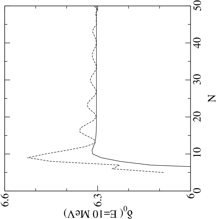
Figure 5.3: Convergence of the scattering phase shift $\delta_{0}(E)$ (in radians) at $E=10$ MeV calculated with (solid line) and without (dashed line) smoothing factors.

5.1.4 Conclusions

In this section we used the Coulomb–Sturmian representation of the Coulomb Green’s operator to solve the Lippmann–Schwinger integral equation with a model nuclear potential describing the interaction of two $\alpha$ particles. In practice this means the approximation of the potential term on a finite subset of this basis. This is the only stage where approximations are made (remember the Green’s operator is calculated analytically), otherwise this method is exact, analytic and provides asymptotically correct solutions. Consequently, bound, resonance and scattering problems can be treated on an equal footing, while these phenomena are usually discussed in rather different ways in conventional quantum mechanical approaches. The unified treatment is also reflected by the fact that all the calculations are made using the same discrete basis, containing also the same basis and other parameters.

Finally, we should call the attention upon the fact that this method is very accurate. Reasonable accuracy is reached already at relatively small basis, around $N=20$. The accuracy gained in larger bases is beyond most of the practical requirements. Test calculations have been performed on a linux PC (Intel PII, 266 MHz) using double precision arithmetic. The calculation of a typical bound or resonant state energy requires the evaluation of the potential matrix by Gauss–Laguerre quadrature and finding the zeros of the determinant (5.16), which incorporates the evaluation of the Coulomb Green’s matrix and the the calculation of a determinant by performing an LU decomposition in each steps. The determination of the energy value in the first column and last row of Table 5.1, which meant $6$ steps in the zero search and handling of $40\times 40$ matrices, took $0.06$ sec. The corresponding resonance energy value in Table 5.2 required $12$ steps in the zero search on the complex energy plane and $0.8$ sec. The evaluation of the three phase shift values in the last row of Table 5.3 took $0.19$ sec., $0.11$ sec. and $0.08$ sec., respectively. So, this method is not only accurate but also very fast.

5.2 An atomic three-body problem

The bound state problem of the Helium atom is investigated as an example of the application of the Faddeev–Merkuriev (FM) integral equations to the atomic three-body problems. The FM equations describing three charged particles interacting through the long-range Coulomb potential are solved using the Coulomb–Sturmian discrete Hilbert space basis representation, which transforms the integral equations into a matrix equation. The solution of the matrix equation is possible due to the analytic representation of a three-body Green’s operator constructed from two independent two-body Green’s operators by performing a convolution integral (Section 2.4).

We recall here that for three-body systems the Faddeev equations [9] are the fundamental equations. Their homogeneous form is fully equivalent to the Schrödinger equation and after one iteration they possess connected kernels, consequently they are, in fact, Fredholm integral equations of second kind. Therefore the Fredholm alternative applies: at certain energy either the homogeneous or the inhomogeneous equations have solutions. Three-body bound states correspond to the solutions of the homogeneous Faddeev equations at real energies.

The Hamiltonian of an interacting three-body system can be written as

$$H=H^{0}+v_{\alpha}+v_{\beta}+v_{\gamma},$$ (5.20)

where $H^{0}$ is the three-body kinetic energy operator and $v_{\alpha}$ denotes the interaction in subsystem $\alpha$ (i.e. the pair interaction of particles $\beta$ and $\gamma$). Here the usual configuration space Jacobi coordinates ${x}_{\alpha}$, ${y}_{\alpha}$ are used, ${x}_{\alpha}$ is the coordinate of the $(\beta,\gamma)$ pair and ${y}_{\alpha}$ is the coordinate of the particle $\alpha$ relative to the center of mass of the pair $(\beta,\gamma)$. Therefore $v_{\alpha}=v_{\alpha}(x_{\alpha})$ represents the interaction of the pair $(\beta,\gamma)$ and depends only on the $x_{\alpha}$ relative coordinate of this pair. In Jacobi coordinates the $H^{0}$ three-body kinetic energy operator is given as a sum of two-body kinetic energy operators

$$H^{0}=h^{0}_{x_{\alpha}}+h^{0}_{y_{\alpha}}=h^{0}_{x_{\beta}}+h^{0}_{y_{\beta}}=h^{0}_{x_{\gamma}}+h^{0}_{y_{\gamma}}.$$ (5.21)

Suppose the $v_{\alpha},v_{\beta},v_{\gamma}$ pair interactions are short-range-type potentials. In this case the Faddeev procedure leads to mathematically sound integral equations for the three-body system. The three-body wave function $|\Psi\rangle$ is decomposed as

$$|\Psi\rangle=|\psi_{\alpha}\rangle+|\psi_{\beta}\rangle+|\psi_{\gamma}\rangle,$$ (5.22)

where the components are defined by

$$|\psi_{i}\rangle=G^{0}v_{i}|\Psi\rangle\qquad\mbox{for}\quad i=\alpha,\beta,\gamma,$$ (5.23)

with the $G^{0}(z)=(z-H^{0})^{-1}$ being the free Green’s operator. For bound states the set of homogeneous Faddeev equations appear as

$$|\psi_{\alpha}\rangle = G_{\alpha}(E)[v_{\alpha}|\psi_{\beta}\rangle+v_{\alpha}|\psi_{\gamma}\rangle]$$ (5.24)

$$|\psi_{\beta}\rangle = G_{\beta}(E)[v_{\beta}|\psi_{\gamma}\rangle+v_{\beta}|\psi_{\alpha}\rangle]$$

$$|\psi_{\gamma}\rangle = G_{\gamma}(E)[v_{\gamma}|\psi_{\alpha}\rangle+v_{\gamma}|\psi_{\beta}\rangle]$$

where $G_{\alpha}(z)=(z-H_{\alpha})^{-1}$ with $H_{\alpha}=H^{0}+v_{\alpha}$. It is proven that the above set of coupled integral equations for short-range potentials have an unique solution.

Unfortunately in the case of the scattering of three charged particles the situation becomes more complicated since the Coulomb potential enters into the game. The Faddeev equations originally were derived for short range interactions and if we simply plug in a Coulomb-like potential they become singular. The solution has been formulated by Faddeev and Merkuriev [38] in a mathematically sound and elegant way via integral equations with connected (compact) kernels and configuration space differential equations with asymptotic boundary conditions.

In practice, however only this latter version of the theory has been applied, since the FM integral equation formulation was too complicated for practical use. Moreover, in bound-state problems only the original version of the Faddeev equations were applied [66, 67, 68] which, in sound mathematical sense, are not well-behaved for Coulomb case and only the bound state nature of the problems helped to overcome the difficulties, however slow convergence in partial wave channels was reported [66, 67]. In order to find a remedy, the equations were solved in total angular momentum representation, which led to three-dimensional equations [68]. So, due to these problems and difficulties, the belief spread that the Faddeev equations are not well-suited for treating atomic three-body problems and other techniques can perform much better, at least for bound states.

Recently, a novel method was proposed by Papp for treating the three-body Coulomb problem via solving the set of Faddeev–Noble and Lippmann–Schwinger integral equations in Coulomb–Sturmian discrete Hilbert space basis representation. The method was elaborated first for bound-state problems [16] with repulsive Coulomb plus nuclear potential, then it was extended for analyzing $p-d$ scattering at energies below the breakup threshold [30]. In these calculations excellent agreements with the results of other well established methods were found and the efficiency and the accuracy of the method were demonstrated. This approach has also been applied to atomic bound-state problems [69]. The Coulomb interactions were split, à la Noble [70], into long-range and short-range terms and the Faddeev procedure was applied only to the short-range potentials. By studying benchmark bound-state problems, contradictory to the conventional approaches, a fast convergence with respect to angular momentum channels was observed. This approach, however, has a limitation which is related to Noble’s splitting. The Noble splitting does not separate the asymptotic channels, so the equations are applicable only in a restricted energy range of low-lying states.

In this section, instead of the Noble splitting, we make use of the mathematically sound Merkuriev splitting of the long-range Coulomb potential [38], and by doing so we solve the Faddeev–Merkuriev integral equations.

5.2.1 Faddeev–Merkuriev integral equations

The fundamental equations for the Coulomb three-body problem is discussed here following Merkuriev ideas. We recall that the Faddeev procedure is based on the observation that the Hamiltonian of the three-body system can be written as the sum of the asymptotically relevant $H^{(l)}$ and irrelevant short-range terms

$$H=H^{(l)}+v_{\alpha}^{(s)}+v_{\beta}^{(s)}+v_{\gamma}^{(s)},$$ (5.25)

where

$$H^{(l)}=H^{0}+v_{\alpha}^{(l)}+v_{\beta}^{(l)}+v_{\gamma}^{(l)}.$$ (5.26)

In equation (5.25) we assumed that the long-range Coulomb potential can be split as

$$v^{C}=v^{(l)}+v^{(s)}$$ (5.27)

by using an appropriate cut-off procedure.

By applying the Faddeev procedure for the short-range part of the potentials we can derive connected kernel integral equations. For this, however it is essential that the asymptotically relevant Hamiltonian $H^{(l)}$ possesses only continuous spectrum. This property guarantees the asymptotic filtering behavior of the Faddeev decomposition [71], and thus the asymptotic orthogonality of the Faddeev components. A potential with an attractive Coulomb tail has infinitely many bound states accumulated at the lower edge of the continuous spectrum, thus the long-range part of an attractive Coulomb potential always has infinitely many bound states. Fortunately, this is true only in the two-body Hilbert space. In a broader space, like the three-body Hilbert space, this statement is not necessarily valid. In the three-body Hilbert space, where we have to consider our potentials, we simply have an extra kinetic energy term, which can modify the character of the spectrum.

Merkuriev proposed to split the Coulomb potential $v_{\alpha}^{C}(x_{\alpha})$ into a short-range and a long-range part by introducing a cut-off function $\zeta_{\alpha}=\zeta_{\alpha}(x_{\alpha},y_{\alpha})$ defined on the three-body configuration space leading to

$$v_{\alpha}^{(s)}(x_{\alpha},y_{\alpha})=v_{\alpha}^{C}(x_{\alpha})\zeta_{\alpha}(x_{\alpha},y_{\alpha}),$$ (5.28)

and

$$v_{\alpha}^{(l)}(x_{\alpha},y_{\alpha})=v_{\alpha}^{C}(x_{\alpha})[1-\zeta_{\alpha}(x_{\alpha},y_{\alpha})].$$ (5.29)

The function $\zeta_{\alpha}$ is constructed in such a way, that it separates the asymptotic two-body sector $\Omega_{\alpha}$ from the rest of the three-body configuration space. On the region of $\Omega_{\alpha}$ the splitting function $\zeta_{\alpha}$ asymptotically tends to $1$ and on the complementary asymptotic region of the configuration space it tends to $0$. Rigorously, $\Omega_{\alpha}$ is defined as a part of the three-body configuration space where the condition

$$|x_{\alpha}|<{y_{\alpha}}_{0}({x_{\alpha}}_{0}+|y_{\alpha}|/{y_{\alpha}}_{0})^{1/\nu},\mbox{with}\quad{x_{\alpha}}_{0},{y_{\alpha}}_{0}>0,\ \nu>2,$$ (5.30)

is satisfied. So, in $\Omega_{\alpha}$ the short-range part $v_{\alpha}^{(s)}$ coincides with the original Coulomb–like potential $v_{\alpha}^{C}$ and in the complementary region vanishes, whereas the opposite holds true for $v_{\alpha}^{(l)}$. A possible functional form for $\zeta$ is given by

$$\zeta(x,y)=2\left\{1+\exp\left[\frac{(x/x_{0})^{\nu}}{1+y/y_{0}}\right]\right\}^{-1},$$ (5.31)

where the parameters $x_{0}$ and $y_{0}$ are rather arbitrary. Fig. 5.4 shows a typical example for the short- and long-range part of an attractive Coulomb potential, respectively. Merkuriev proved that $H^{(l)}$ of Eq. (5.25) with long-range potentials defined in this way possesses only continuous spectrum if the ${x_{\alpha}}_{0}$ and ${y_{\alpha}}_{0}$ parameters for all $\alpha$ fragmentations are chosen big enough (see p. 248 of Ref. [38]).

Now, if we follow the Faddeev procedure with the Merkuriev split of (5.28) and (5.29) we obtain the Faddeev–Merkuriev integral equations

$$|\psi_{\alpha}\rangle=G_{\alpha}^{(l)}(E)[v_{\alpha}^{(s)}|\psi_{\beta}\rangle+v_{\alpha}^{(s)}|\psi_{\gamma}\rangle],$$ (5.32)

where the $G_{\alpha}^{(l)}$ channel Green’s operator is defined as

$$G_{\alpha}^{(l)}(z)=(z-H_{\alpha}^{(l)})^{-1},$$ (5.33)

with

$$H_{\alpha}^{(l)}=H^{(l)}+v_{\alpha}^{(s)}=H^{0}+v^{C}_{\alpha}+v_{\beta}^{(l)}+v_{\gamma}^{(l)}.$$ (5.34)

It is proven [38] that Eqs. (5.32) below the threshold of the continuous spectrum of the Hamiltonian $H$ allow the nontrivial solutions only for discrete set of energy corresponding to the binding energies of an atomic three-body system.

The solution of the Faddeev equations (5.24) and(5.32) necessitates the determination of the asymptotically relevant Green’s operator in some basis representation. This can be done using convolution integral technique of Section 2.4.

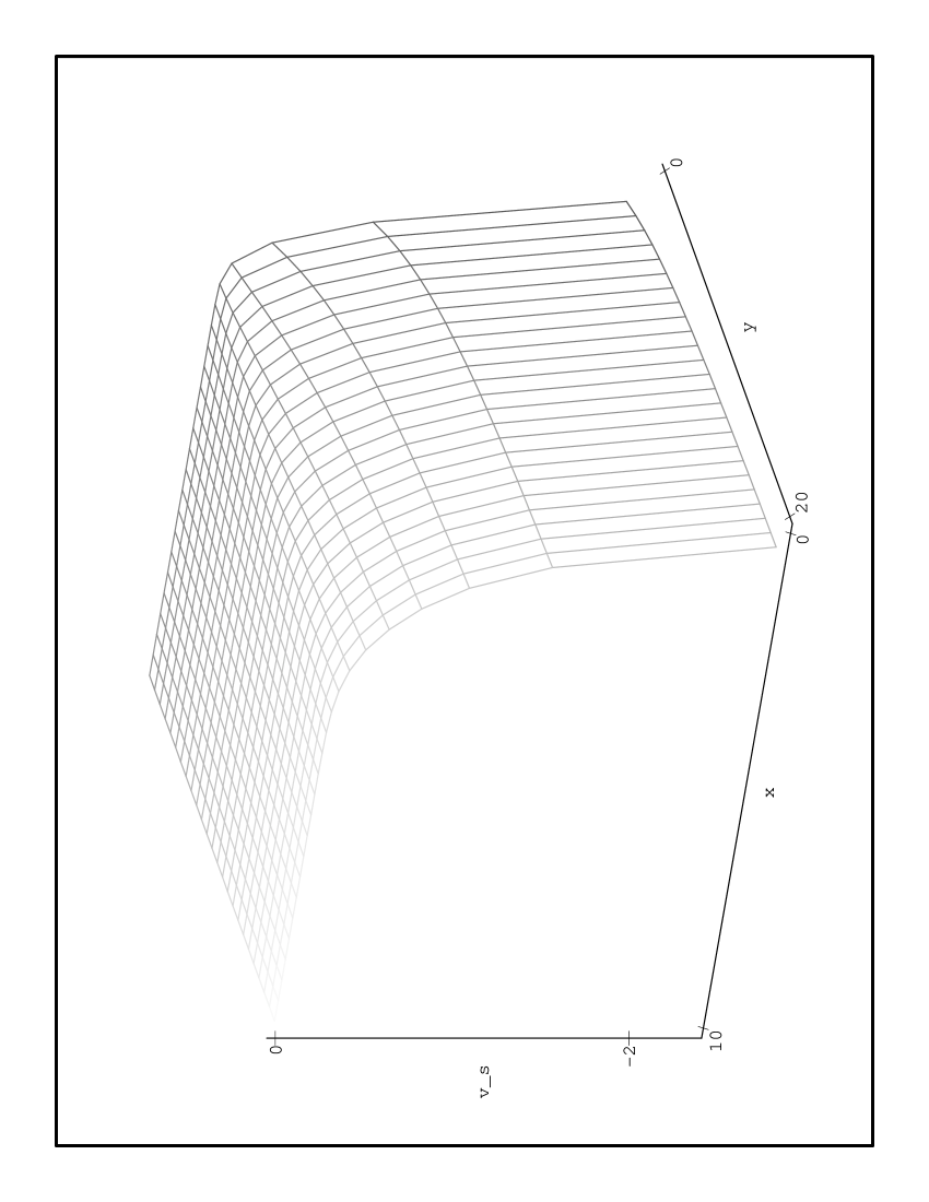
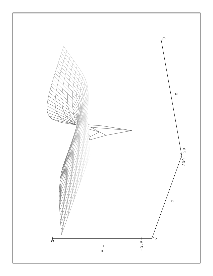
$v^{(s)}$	$v^{(l)}$

Figure 5.4: The short- and the long-range part of an attractive Coulomb potential in the $(x,y)$ three-body configuration space with parameters $x_{0}=1$, $y_{0}=5$ and $\nu=2.2$ of $\zeta$ defined in Eq. (5.31).

5.2.2 Solution in Coulomb–Sturmian space representation

The three-body Hilbert space is a direct product of two-body Hilbert spaces, so an appropriate discrete basis in the three-body Hilbert space can be constructed as the angular momentum coupled direct product of the (4.25) Coulomb–Sturmian basis functions as

$$|n\nu l\lambda\rangle_{\alpha}=[|nl\rangle_{\alpha}\otimes|\nu\lambda\rangle_{\alpha}],\ \ \ \ (n,\nu=0,1,2,\ldots),$$ (5.35)

where $l$ and $\lambda$ denote the angular momenta associated with the coordinates $x$ and $y$, respectively, and the bracket stands for angular momentum coupling. With this basis the completeness relation takes the form (with angular momentum summation implicitly included)

$${\bf 1}=\lim\limits_{N\to\infty}\sum_{n,\nu=0}^{N}|\widetilde{n\nu l\lambda}\rangle_{\alpha}\;\mbox{}_{\alpha}\langle{n\nu l\lambda}|=\lim\limits_{N\to\infty}{\bf 1}^{N}_{\alpha}.$$ (5.36)

It should be noted that in the three-body Hilbert space three equivalent bases belonging to fragmentation $\alpha$, $\beta$ and $\gamma$ are possible.

In Eqs. (5.32) we introduce the approximation

$$|\psi_{\alpha}\rangle=G_{\alpha}^{(l)}(z){\bf 1}^{N}_{\alpha}v^{(s)}_{\alpha}\sum_{\gamma\neq\alpha}{\bf 1}^{N}_{\gamma}|\psi_{\gamma}\rangle,$$ (5.37)

i.e. the short-range potential $v_{\alpha}^{(s)}$ in the three-body Hilbert space is taken in the separable form

$$v_{\alpha}^{(s)}\approx\sum_{n,\nu,n^{\prime},\nu^{\prime}=0}^{N}|\widetilde{n\nu l\lambda}\rangle_{\alpha}\;\underline{v}_{\alpha\beta}^{(s)}\;\mbox{}_{\beta}\langle\widetilde{n^{\prime}\nu^{\prime}l^{\prime}\lambda^{\prime}}|,$$ (5.38)

where $\underline{v}_{\alpha\beta}^{(s)}=\mbox{}_{\alpha}\langle n\nu l\lambda|v_{\alpha}^{(s)}|n^{\prime}\nu^{\prime}l^{\prime}{\lambda}^{\prime}\rangle_{\beta}$. These matrix elements can be calculated numerically by making use of the transformation of Jacobi coordinates. The ket and bra states are defined for different fragmentation, depending on the environment of the potential operators in the equations.

Now, with this approximation, the solution of the homogeneous Faddeev–Merkuriev integral equations turns into the solution of a matrix equation for the component vector $\underline{\psi}_{\alpha}=\mbox{}_{\alpha}\langle\widetilde{n\nu l\lambda}|\psi_{\alpha}\rangle$

$$\underline{\psi}_{\alpha}=\underline{G}_{\alpha}^{(l)}(z)\underline{v}^{(s)}_{\alpha}\sum_{\gamma\neq\alpha}\underline{\psi}_{\gamma},$$ (5.39)

where $\underline{G}_{\alpha}^{(l)}=\mbox{}_{\alpha}\langle\widetilde{n\nu l\lambda}|G_{\alpha}^{(l)}|\widetilde{n^{\prime}\nu^{\prime}l^{\prime}{\lambda}^{\prime}}\rangle_{\alpha}.$ A unique solution exists if and only if

$$\det\{[\underline{G}^{(l)}(z)]^{-1}-\underline{v}^{(s)}\}=0.$$ (5.40)

The solution of the above matrix equation requires the determination of the Coulomb–Sturmian representation of the three-body Green’s operator ${G}_{\alpha}^{(l)}$ of Eq. (5.33). Normally this task necessitates the solution of Faddeev-type integral equations or a triad of Lippmann–Schwinger integral equations [73]. However, the Hamiltonian $H_{\alpha}^{(l)}$ has the peculiar property, that it supports bound state only in the subsystem $\alpha$, and thus there is only one kind of asymptotic channel, the $\alpha$ channel. For such a system, if the asymptotics is treated properly, one single Lippmann–Schwinger equation is sufficient for an unique solution [72]. Merkuriev proposed an appropriate Lippmann-Schwinger equation which provides a unique solution for ${G}_{\alpha}^{(l)}$

$$G_{\alpha}^{(l)}(z)=G_{\alpha}^{as}(z)+G_{\alpha}^{as}(z)V^{as}_{\alpha}G_{\alpha}^{(l)}(z),$$ (5.41)

where the three-body potential $V_{\alpha}^{as}$ is defined such that it decays faster than the Coulomb potential in all direction of the three-body configuration space. The operators $G_{\alpha}^{as}$ and $V^{as}_{\alpha}$ are complicated three-body operators, and to construct them, Merkuriev used different approximation schemes in different regions of the configuration space.

It is important to realize that in our approach to get the solution only matrix elements of ${G}_{\alpha}^{(l)}$ between finite number of square integrable CS functions are needed. That is the reason why the matrix elements of the channel Green’s operator can be obtained as

$$\underline{G}_{\alpha}^{(l)}(z)=\underline{\widetilde{G}}_{\alpha}(z)+\underline{\widetilde{G}}_{\alpha}(z)\underline{U}^{\alpha}\underline{G}_{\alpha}^{(l)}(z),$$ (5.42)

where

$$\underline{\widetilde{G}}_{\alpha}=\mbox{}_{\alpha}\langle\widetilde{n\nu l\lambda}|\widetilde{G}_{\alpha}|\widetilde{n^{\prime}\nu^{\prime}l^{\prime}{\lambda}^{\prime}}\rangle_{\alpha},\quad\underline{U}^{\alpha}=\mbox{}_{\alpha}\langle{n\nu l\lambda}|U^{\alpha}|{n^{\prime}\nu^{\prime}l^{\prime}{\lambda}^{\prime}}\rangle_{\alpha},$$ (5.43)

with $\widetilde{G}_{\alpha}(z)=(z-\widetilde{H}_{\alpha})^{-1}$ and $U^{\alpha}=H_{\alpha}^{(l)}-\widetilde{H}_{\alpha}$. The channel-distorted long-range Hamiltonian $\widetilde{H}_{\alpha}$ is defined as

$$\widetilde{H}_{\alpha}=h_{x_{\alpha}}^{C}+h_{y_{\alpha}}^{(l)},$$ (5.44)

where $h_{x_{\alpha}}^{C}=h_{x_{\alpha}}^{0}+v_{\alpha}^{C}$ is the two-body Coulomb Hamiltonian.

Since $H_{\alpha}^{(l)}$ does not generate rearrangement channels, we should define $h_{y_{\alpha}}^{(l)}$ such that $\widetilde{H}_{\alpha}$ also preserve this property. If we are dealing with repulsive Coulomb interactions, i.e. $e_{\alpha}(e_{\beta}+e_{\gamma})\geq 0$, this requirement can be easily fulfilled and $h_{y_{\alpha}}^{(l)}$ is defined by

$$h_{y_{\alpha}}^{(l)}=h_{y_{\alpha}}^{C}=h_{y_{\alpha}}^{0}+{e_{\alpha}(e_{\beta}+e_{\gamma})}/{y_{\alpha}}$$ (5.45)

and $U^{\alpha}$ takes the form

$$U^{\alpha}=v_{\beta}^{(l)}+v_{\gamma}^{(l)}-{e_{\alpha}(e_{\beta}+e_{\gamma})}/{y_{\alpha}}.$$ (5.46)

On the other hand, in the case of an attractive interaction, like the Helium atom where $e_{\alpha}(e_{\beta}+e_{\gamma})<0$, the attractive Coulomb tail of $h_{y_{\alpha}}^{C}$ generate infinitely many bound states which has to be pushed away from the spectrum. In practice this is achieved by introducing a repulsive Gaussian term into (5.46)

$$U^{\alpha}=v_{\beta}^{(l)}+v_{\gamma}^{(l)}-\Lambda\exp(-\kappa y_{\alpha}^{2})-{e_{\alpha}(e_{\beta}+e_{\gamma})}/{y_{\alpha}},$$ (5.47)

where $\Lambda$ and $\kappa$ are free parameters. Now the (5.43) matrix elements of $U^{\alpha}$ can easily be calculated numerically applying basis functions from the same fragmentations on both sides.

We note here that an alternative and mathematically more sound procedure for removing the bound states generated by the attractive Coulomb potential is being under development. The basic idea of the new procedure is the application of projection operators constructed as convolution integrals of Green’s operators.

The most crucial point in the solution of Eq. (5.42) is the calculation of the matrix elements $\underline{\widetilde{G}}_{\alpha}$. The operator $\widetilde{G}_{\alpha}$ is a resolvent of the sum of two commuting Hamiltonians, $h^{C}_{x_{\alpha}}$ and $h_{y_{\alpha}}^{(l)}$ according to (5.44), which act in different two-body Hilbert spaces. As it was discussed in Section 2.4, the three-body Green’s operator $\widetilde{G}_{\alpha}$ equates to a convolution integral of two-body Green’s operators, i.e.

$$\widetilde{G}_{\alpha}(z)=\frac{1}{2\pi\mathrm{i}}\oint_{C}dz^{\prime}\,g^{C}_{x_{\alpha}}(z-z^{\prime})\;g_{y_{\alpha}}^{(l)}(z^{\prime}),$$ (5.48)

where $g^{C}_{x_{\alpha}}(z)=(z-h^{C}_{x_{\alpha}})^{-1}$ and $g_{y_{\alpha}}^{(l)}(z)=(z-h_{y_{\alpha}}^{(l)})^{-1}$. The contour $C$ should be taken such that it encircles the continuous spectrum of $h_{y_{\alpha}}^{(l)}$ so that $g^{C}_{x_{\alpha}}$ is analytic on the domain encircled by $C$. For bound state problems this requirement can easily be fulfilled (see Fig. (5.5)). The matrix elements $\underline{\widetilde{G}}_{\alpha}$ of Eq. (5.43) can be cast into the convolution integral of the outer product of the corresponding matrices

$$\underline{\widetilde{G}}_{\alpha}(z)=\frac{1}{2\pi\mathrm{i}}\oint_{C}dz^{\prime}\,_{\alpha}\langle\widetilde{nl}|g^{C}_{x_{\alpha}}(z-z^{\prime})|\widetilde{n^{\prime}l^{\prime}}\rangle_{\alpha}{}_{\alpha}\langle\widetilde{\nu\lambda}|g_{y_{\alpha}}^{(l)}(z^{\prime})|\widetilde{\nu^{\prime}\lambda^{\prime}}\rangle_{\alpha}.$$ (5.49)

The great advantage of using CS basis is that on this basis the matrix elements of the two-body Green’s operators are given analytically on the whole complex plane (see Section 4.2), thus the convolution integral can be performed in practice.

Figure 5.5: Contour $C$ for the convolution integral of Eq. (5.48). The contour $C$ encircles the (continuous) spectrum of $g^{(l)}_{y_{\alpha}}$ and avoids the singularities of $g^{C}_{x_{\alpha}}$.

As an application, the binding energy of the Helium atom (with an infinitely massive core) is determined as the three-body energy to be obtained from equation (5.40). The convergence of the binding energy with respect to $N$, the number of basis states in the approximation of Eq. (5.37), is shown in Table 5.4. Excellent convergence is achieved up to $6-7$ significant digits with $N\sim 19$ applied for $n$ and $\nu$. In Table 5.4, for comparison, we also quote the result of a very accurate variational calculation.

$N$	$l=0$	$l=4$
10	2.897586	2.903741
11	2.897591	2.903746
12	2.897593	2.903746
13	2.897593	2.903746
14	2.897593	2.903746
15	2.897593	2.903746
16	2.897593	2.903746
17	2.897593	2.903745
18	2.897593	2.903745
19	2.897593	2.903745
Variational calculation in ref. [74]		2.903724376984

Table 5.4: Convergence of the binding energy of the Helium atom. $N$ denotes the maximum value of $n$ and $\nu$, i.e. the number of employed basis states. The quoted energy values are given in atomic units $(\hbar=m_{e}=e^{2}=1)$. Angular momentum states have been taken into account up to $l=0$ and $l=4$. The values $b=5$, $\kappa=2$, $\Lambda=5$ are chosen for the CS basis and the (5.47) repulsive Gaussian parameters respectively. The Merkuriev parameters of the splitting function of Eq. (5.31) are $x_{0}=0.7$, $y_{0}=15$ and $\nu=2.2$ respectively.

Summary

In this work we have presented a rather general and easy-to-apply method for discrete Hilbert space representation of quantum mechanical Green’s operators. We have shown that if in some discrete Hilbert space basis representation the Hamiltonian takes an infinite symmetric tridiagonal, i.e. Jacobi-matrix form the corresponding Green’s matrix can be calculated on the whole complex energy plane by a continued fraction. The procedure necessitates only the analytic calculation of the Hamiltonian matrix elements, which are used to construct the coefficients of the continued fraction. This continued fraction representation of the Green’s operator was shown to be convergent for the bound state energy region. The theory of analytic continuation of continued fractions was utilized to extend the representation to the whole complex energy plane. The presented method provides a simple, easily applicable and analytically correct recipe for calculating discrete basis representation of Green’s operators.

The general procedure was applied to determine matrix representation of specific Green’s operators. The D-dimensional Coulomb Hamiltonian was shown to possess a Jacobi-matrix structure on the Coulomb–Sturmian basis. The tridiagonal matrix elements of the Hamiltonian were used to construct the continued fraction representation of the Coulomb Green’s operator. Numerical tests on the convergence of the continued fraction and on the effect of the analytic continuation were presented on this example. Continued fraction representation of relativistic Green’s operators corresponding to the Klein–Gordon and the second order Dirac equation could be determined because of the Jacobi-matrix structure of the relativistic Hamiltonians on the relativistic Coulomb–Sturmian basis. The relativistic energy spectra of the hydrogen-like atoms are calculated as the poles of the relativistic Coulomb Green’s operator and demonstrate the high precession numerical accuracy of our continued fraction representation. The method has been applied for the D-dimensional harmonic oscillator, as well. As a non-trivial example the generalized Coulomb potential, which is a member of the exactly solvable Natanzon confluent potential class, is considered. The radial Hamiltonian containing this potential exhibits a tridiagonal form with analytically known matrix elements on the generalized Coulomb–Sturmian basis, so our procedure is also applicable here.

Once the representation of the Green’s operator in a discrete basis is available we can proceed to solve few-body integral equations which provide the real test field for our Green’s operator in respect of its practical applicability and importance.

The continued fraction representation of the Coulomb–Sturmian space Coulomb Green’s operator is used for giving a unified solution of the two-body Lippmann–Schwinger equation for the bound, resonant and scattering states. The performance of this approach is illustrated by the detailed investigation of a model nuclear potential describing the interaction of two $\alpha$ particles.

As a second application the Faddeev–Merkuriev equations are solved for an atomic three-body bound state problem. The solution method requires the evaluation of a three-body Green’s operator, wich is done by performing a convolution integral of two-body Coulomb Green’s operators. This convolution integral represents the real test for our Green’s matrices calculated by continued fractions over the whole complex plane.

We can conclude that our general, readily computable and numerically exact continued fraction method for determining discrete Hilbert space representation of Green’s operators is turned out to be valuable in solving few-body problems.

Összefoglalás
(The Hungarian summary of the thesis.)

Előzmények

A bennünket körülvevő fizikai világ mikroszkopikus leírását két különböző irányból kísérelhetjük meg. Soktest vagy térelméleti módszereket követve a sok, illetve végtelen szabadsági fokkal rendelkező fizikai rendszereket mint statisztikus sokaságokat kezelhetjük. Ezzel szemben a néhánytest fizika célja az olyan kevés szabadsági fokkal rendelkező rendszerek vizsgálata, ahol az egymással kölcsönható objektumok viselkedésének minél teljesebb fizikai megismerését még reális célként fogalmazhatjuk meg. A kvantummechanikai néhánytest rendszerek elméleti tanulmányozása központi szerepet tölt be mind az atom-, a mag- és a részecskefizika fejlődésében, hisz az alapvető természeti törvények megismeréséhez nélkülözhetetlenek a néhánytest modellek.

A kvantummechanikai néhánytest probléma alapvető egyenletei, mint például a Lippmann–Schwinger- és a Fagyejev-egyenletek, általában integrálegyenletek. Néhánytest fizikában az integrálegyenletek használata a differenciálegyenletek helyett többek közt azzal az előnnyel jár, hogy a megoldandó egyenletek automatikusan tartalmazzák a dinamika szempontjából alapvető határfeltételeket. Éppen ez az oka annak, hogy a bonyolult aszimptotikus határfeltételekkel jellemezhető szórási problémák tanulmányozása során az integrálegyenletek jelentős előnyt élveznek. Azonban a legtöbb gyakorlati alkalmazás esetében az integrálegyenleteket, azok előnyös tulajdonságai ellenére, mellőzik és helyettük inkább a megfelelő Schrödinger-egyenlet valamely alkalmas közelítését használják. Ennek oka abban keresendő, hogy az integrálegyenletek a Hamilton-operátor helyett annak rezolvensét a Green-operátort tartalmazzák. A Green-operátor meghatározása pedig jóval bonyolultabb feladat mint a megfelelő Hamilton-operátor közelítése.

Egy adott kvantummechanikai néhánytest rendszer teljes Green-operátorának meghatározása ekvivalens a probléma teljeskörű megoldásával, ugyanis a Green-operátor hordozza a fizikai rendszerről nyerhető összes információt. Többek között a rendszer energiasajátértékei, kötött, rezonancia- és szórási állapotai, hullámfüggvénye, állapotsűrűsége valamint időbeli fejlődése határozható meg a Green-operátor valamely reprezentációja ismeretében.

A legalapvetőbb néhánytest rendszerek, mint pl. a szabad részecske, a harmonikus oszcillátor vagy a Coulomb-térben mozgó töltött részecske, Green-operátorának valamely reprezentációja az irodalomból már ismert [19, 20, 22, 25]. Ezen operátorok számolását az alkalmasan választott reprezentáció (momentum saját vektorok, harmonikus oszcillátor függvények, Coulomb–Strum-függvények) valamint a matematika speciális függvényeinek bizonyos feltételek melletti intenzív használata tette lehetővé.

A Green-operátorok analitikus ismerete képezi az alapját egy, az utóbbi időben kifejlesztett kvantummechanikai közelítő módszernek is [23]. A módszer során a Hamilton-operátor aszimptotikusan meghatározó tagjainak (kinetikus energia operátor, hosszú hatótávolságú kölcsönhatások) megfelelő Green-operátort egzaktul analitikusan számolják, és csupán az aszimptotikusan irreleváns rövid hatótávolságú potenciált közelítik egy szeparábilis kifejtéssel a Hilbert-tér egy csonkolt bázisán (a módszer ezért kapta a PSE, Potential Separable Expansion elnevezést). A hosszú hatótávolságú tagok egzakt kezelése biztosítja a megoldások aszimptotikusan korrekt voltát. A módszert sikeresen alkalmazták a kéttest rendszereket leíró Lippmann–Schwinger- [24, 25, 27, 28], valamint a háromtest rendszerek alapvető egyenleteit jelentő Fagyejev-egyenletek megoldására [16]. A módszer alkalmazása során a Fagyejev-egyenletek esetében a legnagyobb kihívást egy háromtest Green-operátor számolása jelenti, melyet kéttest Green-operátorok konvolúciós integráljaként állítanak elő.

Mindezek miatt állíthatjuk, hogy valamely rendszer Green-operátorának analitikus előállítása a kvantummechanikai néhánytest problémák megoldása szempontjából nagy jelentőséggel bír.

Eredményeim

Doktori munkám során kidolgoztam egy általános, egyszerűen megvalósítható, numerikusan stabil analitikus módszert a kvantummechanikai Green-operátorok diszkrét Hilbert-térbeli reprezentációjának lánctörtes előállítására. A módszer alapját az a felismerés képezi, hogy amennyiben a rendszer Hamilton-operátora valamely diszkrét Hilbert-tér bázison végtelen szimmetrikus tridiagonális mátrix, azaz Jacobi-mátrix, akkor a megfelelő Green-mátrix egy tetszőleges véges almátrixa a tridiagonális Hamilton mátrixelemekből és egy lánctörtből számolható. A lánctört együtthatóit szintén a Jacobi-mátrixelemekből nyerhetjük [31].

Továbbá a kötöttenergia-tartományban a Green-operátor mátrixelemei egy háromtagú rekurziós reláció minimális megoldásaiként adódnak, ami Pincherle tétele alapján biztosítja a Green-operátor lánctörtes előállításának konvergens voltát ezen a tartományon.

A komplex energia-sík szórási és rezonancia tartományaiban a Green-operátor lánctörtes reprezentációját a kötött tartományon konvergens lánctört analitikus folytatásával adtam meg. Erre azért volt szükség, mert ezen energiaértékeknél a Green-mátrixelemek már nem minimális megoldásai a rekurziónak, s így az eredeti lánctört nem, hanem csak annak analitikus folytatása konvergens. Az analitikusan folytatott lánctörttel a Green-operátor teljes komplex sikon vett analitikus reprezentációját állítottam elő.

Numerikus szempontból fontos felismerést jelentett az, hogy az analitikusan folytatott lánctört konvergenciájának sebességét és numerikus stabilitását a lánctörtek Bauer-Muir transzformációjának [41] többszörös alkalmazása jelentősen javítja.

Felhasználva, hogy a megfelelő bázison az alábbi rendszerek Hamilton operátora tridiagonális szerkezetű, a kifejlesztett általános módszert alkalmaztam a következő Green-operátorok diszkrét bázison történő lánctörtes reprezentációjának előállítására:

• D-dimenziós Coulomb-probléma Green-operátora a Coulomb–Sturm-bázison,

• D-dimenziós harmonikus oszcillátor Green-operátora a harmonikus oszcillátor függvények bázisán,

• Általánosított Coulomb-potenciál Green-operátora az általánosított Coulom–Sturm-bázison,

• Relativisztikus Coulomb–Green-operátorok, azaz a Klein–Gordon- és a másodrendű Dirac-egyenlet, a relativisztikus Coulomb–Sturm-bázison.

Az analitikusan számolt lánctörtes Green-operátorokat a két- illetve háromtest problémák integrálegyenleteinek megoldására szolgáló kvantummechanikai közelítő módszerekben teszteltem, ezáltal bizonyítva a lánctörtes Green-operátorok gyakorlati alkalmazhatóságát:

• A Coulomb–Green-operátor Coulomb–Sturm reprezentációjának lánctörtes előállítását használtam fel a Coulomb–Sturm-bázisú PSE módszer alkalmazása során egy, az alfa részecskék kölcsönhatását leíró magfizikai modellpotenciált tartalmazó kéttest Lippmann–Schwinger-integrálegyenlet megoldására [34].

• Egy, a Fagyejev–Merkuriev háromtest integrálegyenletek megoldására szolgáló közelítő módszerben alkalmaztam a lánctörtes Coulomb–Green-operátort egy atomfizikai háromtest probléma kötött állapoti megoldása során.

Munkám során a matematikai fizika és a néhánytest kvantummechanika módszereit alkalmaztam, és eredményeim a néhánytest módszerekkel leírható atom-, mag- és részecskefizika területén alkalmazhatóak. Lehetőséget látok arra is, hogy a tridiagonális mátrixok és a lánctörtek használatát jelentő alapötlet a fizika más területein is sikerrel alkalmazható legyen.

References

- [1] A. L. Fetter and J. D. Walecka, Quantum Theory of Many-Particle Systems (McGRAW-HILL, 1971).
- [2] M. Kaku, Quatum Field Theory, a Modern Introduction (Oxford University Press, New York, 1993).
- [3] F. Mandl and G. Shaw, Quantum Field Theory, Revised Edition (John Wiley & Sons, New York, 1993).
- [4] T. C. Griffith, E. A. Power, editors, Nuclear forces and the few-nucleon problem. Proceedings of the international conference held at the physics department, University College, London, on 8-11 July 1959 (Pergamen Press, Oxford, 1960).
- [5] E. A. Hylleraas, Z. Phys. 54, 347-366 (1929).
-
[6]
C. L. Pekeris, Phys. Rev. 112, 1649-1658 (1958);
C. L. Pekeris, Phys. Rev. 115, 1216-1221 (1959). - [7] B. A. Lippmann and J. Schwinger, Variational principles for scattering processes, Phys. Rev. 79, 469-480 (1950).
- [8] M. Gell-Mann and M. L. Goldberger, The former theory of scattering, Phys. Rev. 91, 398-408 (1953).
- [9] L. D. Faddeev, Scattering theory for a three-particle system, Zh. Eksp. Teor. Fiz. 39, 1459-1467 (1960).
- [10] J. W. Humberston, R. L. Hall and T. A. Osborn, Bound states of three identical bosons, Phys. Lett. 27B, 195-198 (1968).
- [11] C. Gignoux and A. Laverne, Three-nucleon bound state from Faddeev equations with a realistic potential, Phys. Rev. Lett. 29, 436-438 (1972).
- [12] W. Glöckle, H. Witała, D. Hüber, H. Kamada and J.Golak, Phys. Rep. 274, 107 (1996).
-
[13]
G. L. Payne, J. L. Friar, B. F. Gibson and I. R. Afnan,
Phys. Rev. C 22, 823-831 (1980);
G. L. Payne, J. L. Friar and B. F. Gibson, Phys. Rev. C 26, 1385-1398 (1982);
C. R. Chen, G. L. Payne, J. L. Friar and B. F. Gibson, Phys. Rev. C 31, 2266-2273 (1985). -
[14]
M. Fabre de la Ripelle,
Ann. Phys. 147, 281 (1983);
J. Avery, Hyperspherical Harmonics, Application in Quantum Theory (Kluwer, Dordrecht, 1989);
C. D. Lin, Phys. Rep. 257, 1 (1995). -
[15]
J. Carlson,
Phys. Rev. C36, 2026 (1987);
B. L. Hammond, W. A. Lester, Jr. and P. J. Reynolds, Monte Carlo Methods in Ab Inito Quantum Chemistry (World Scientific, Singapore, 1994). -
[16]
Z. Papp and W. Plessas,
Phys. Rev. C, 54, 50 (1996);
Z. Papp, Few-Body Systems, 24 263 (1998). - [17] K. Varga, Stochastic Variational Approach to Quantum-Mechanical Few-Body Problems (Springer-Verlag Berlin, Heidelberg, Lecture Notes in Physics, 1998).
-
[18]
M. D. Scadron,
Advanced Quantum Theory
(Springer-Verlag, Heidelberg, 1979);
J. J. Sakurai, Modern Quantum Mechanics (The Benjamin/Cummings Publishing Co. Inc., 1985). - [19] R. G. Newton, Scattering Theory of Waves and Particles (Springer, New York, 1982).
- [20] J. R. Taylor, Scattering Theory: The Theory on Nonrelativistic Collisions (John Wiley & Sons, New York, 1972).
- [21] M. Moshinsky, The Harmonic Oscillator in Modern Physics: From Atoms to Quarks, Contemporary Concepts in Physics Series (Gordon & Breach Science Pub., Revised edition, 1996).
- [22] G. L. Bayne and L. Schlessinger, J. Comp. Phys. 266, 13 (1973).
- [23] J. Révai, JINR Preprint E4-9429, Dubna, 1975.
-
[24]
F. A. Gareev, M. Ch. Gizzatkulov, J. Révai,
Nucl. Phys. A 286 512 (1977);
E. Truhlik, Nucl. Phys. A 296 134 (1978);
F. A. Gareev, S. N. Ershov, J. Révai, J. Bang, B. S. Nillsson, Phys. Scripta 19, 509 (1979);
B. Gyarmati, A. T. Kruppa and J. Révai, Nucl. Phys. A 326, 119 (1979);
B. Gyarmati, A. T. Kruppa, Nucl. Phys. A 378, 407 (1982);
B. Gyarmati, A. T. Kruppa, Z. Papp and G. Wolf, Nucl. Phys. A 417, 393 (1984);
A. T. Kruppa and Z. Papp, Comp. Phys. Comm. 36, 59 (1985);
J. Révai, M. Sotona and J. Žofka, J. Phys. G: Nucl. Phys. 11, 745 (1985);
K. F. Pál, J. Phys. A: Math. Gen. 18, 1665 (1985). - [25] Z. Papp, J. Phys. A 20, 153 (1987).
-
[26]
B. A. Zon, N. L. Manakov and L. P. Rapoport,
Sov. Phys.-JETP 28, 480 (1969);
R. N. Hill and B. D. Huxtable, J. Math. Phys. 23, 2365 (1982). - [27] Z. Papp, Phys. Rev. C 38, 2457 (1988).
- [28] Z. Papp, Phys. Rev. A 46, 4437 (1992).
-
[29]
Z. Papp,
Comp. Phys. Comm. 70, 426 (1992);
ibid. 70, 435 (1992). - [30] Z. Papp, Phys. Rev. C, 55, 1080 (1997).
- [31] B. Kónya, G. Lévai and Z. Papp, Green’s matrix from Jacobi matrix Hamiltonian, J. Math. Phys. 38, 4832 (1997).
- [32] G. Lévai, B. Kónya and Z. Papp, Unified treatment of the Coulomb and harmonic oscillator potentials in D dimensions, J. Math. Phys. 39, 5811 (1998).
- [33] B. Kónya and Z. Papp, On the Coulomb–Sturmian matrix elements of relativistic Coulomb Green’s operators, J. Math. Phys. 40, 2307 (1999).
- [34] B. Kónya, G. Lévai and Z. Papp, Continued fraction representation of the Coulomb Green’s operator and unified description of bound, resonant and scattering states, Phys. Rev. C 61, 034302 (2000).
- [35] R. D. Richtmyer, Principles of Advanced Mathematical Physics (Springer-Verlag, New York, 1978).
- [36] N. Dunford and J. Schwartz, Linear Operators I. (Interscience, New York, 1958).
- [37] L. Bianchi and L. Favella, Nuovo Cim. 6, 6873 (1964).
- [38] L.D. Faddeev and S.P. Merkuriev, Quantum Scattering Theory for Several Particle Systems (Kluver, Dordrech, 1993).
- [39] G.H. Golub and C.F. van Loan, Matrix Computations (John Hopkins University Press, Baltimore, 1983).
- [40] P. Rózsa, Linear Algebra and Its Applications, (in Hungarian) (Műszaki Könyvkiadó, Budapest 1976).
- [41] L. Lorentzen and H. Waadeland, Continued Fractions with Applications (North-Holland, Amsterdam, 1992).
- [42] W. B. Jones and W. J. Thron, Continued Fractions: Analytic Theory and Applications (Addison-Wesley, Reading, 1980).
- [43] C. Lanczos, J. Res. Nat. Bur. Stand., 45, 255 (1950).
- [44] Husi otlete !!!!!!!!!!!!
- [45] W. Gautschi, Computational aspects of three-term recurrence relations SIAM Review 9, 24 (1967).
- [46] R. Bombelli, L’Algebra (Venezia, 1572).
- [47] W. J. Thron and H. Waadeland, Accelerating convergence of limit periodic continued fractions Numer. Math. 34, 155 (1980).
- [48] H. Waadeland, Det Kgl. Norske Vid. Selsk. Skr. 9, 1 (1966).
- [49] D. Masson, The rotating harmonic oscillator eigenvalue problem. 1. Continued fractions and analytic continuation J.Math. Phys. 24, 2074 (1983).
- [50] G. Bauer, Abh. der Kgl. Bayr. Akad. der Wiss., Munchen, Zweite Klasse, 11, 99 (1872).
- [51] T. Muir, A theorem in continuants Phil. Mag., 3, 137 (1877).
- [52] S. Pincherle, Delle funzioni ipergeometriche e di varie questioni ad esse attinenti Giorn. Mat. Battaglini 32, 209 (1894). (also in Opere Selecte, Vol. 1, 273-357)
- [53] S. Ramanujan, “Notebook”, Vol. 2, Tata Institute of Fundamental Research, Bombay, (1957).
- [54] E. J. Heller, Phys. Rev. A 12, 1222 (1975).
- [55] V. A. Kostelecký, M. M. Nieto and D. R. Truax, Phys. Rev. D 32, 2627 (1985).
- [56] M. Abramowitz and I. Stegun, Handbook of Mathematical Functions (Dover, New York, 1970).
-
[57]
M. Rotenberg,
Ann. Phys. (N.Y.) 19, 262 (1962);
M. Rotenberg, Adv. At. Mol. Phys. 6, 233 (1970). - [58] L. C. Hostler, J. Math. Phys. 28, 2984 (1987).
-
[59]
A. Khare,
Fractional Statistics and Quantum Theory
(World Scientific Pub. Co., 1996);
A. Lerda, Anyons : Quantum Mechanics of Particles With Fractional Statistics, Lecture Notes in Physics (Springer Verlag, 1993). - [60] G. Lévai and B. W. Williams, J. Phys. A 26, 3301 (1993).
- [61] P. Cordero and S. Salamó, J. Phys. A 24, 5299 (1991).
- [62] E. W. Schmid, G. Spitz and W. Lösch, Theoretical Physics on the Personal Computer, Chapter 13 (Springer, Berlin, 1988).
- [63] C. Lanczos, Linear Differential Operators (D. van Nostrand, London, 1961).
- [64] I. Borbély, private communication in Ref.[23], 1975. The factors were subsequently used in all calculations of Refs. [23, 24, 25, 27, 28, 29, 16, 30].
- [65] F. Ajzenberg-Selove, Nucl. Phys. A 490, 1 (1988).
-
[66]
E. Cravo, A. C. Fonseca,
Few-Body Systems 5, 117 (1988);
A. C. Fonseca, M. T. Peña, Phys. Rev. A 38, 4967 (1988). -
[67]
N. W. Schellingerhout, L. P. Kok, G .D. Bosveld,
Phys. Rev. A. 40, 5568 (1989);
N. W. Schellingerhout, L. P. Kok, Nucl. Phys. A. 508 299c (1990). -
[68]
A. A. Kvitsinsky, C.-Y. Hu, J. Carbonell,
C. Gignoux, S. P. Merkuriev,
Few-Body Systems, Suppl. 6, 544 (1992);
C.-Y. Hu, A. A. Kvitsinsky, S. P. Merkuriev, Phys. Rev. A. 45, 2723 (1992);
A. A. Kvitsinsky, C.-Y. Hu, Few-Body Systems 12 7 (1992);
A. A. Kvitsinsky, Hyperfine Interactions 82, 59 (1993). - [69] Z. Papp, Few-Body Systems 24, 263 (1998).
- [70] J. V. Noble, Phys. Rev. 161, 945 (1967).
- [71] V. Vanzani, Few-Body Nuclear Physics, (IAEA Vienna), 57 (1978).
- [72] W. Sandhas, Few-Body Nuclear Physics, (IAEA Vienna), 3 (1978).
- [73] W. Glöckle, Nucl. Phys. A 141, 620 (1970).
- [74] A. Yeremin, A. M. Florov, E. B. Kutukova, Few-Body Systems 4, 111 (1988).