Quantum effects after decoherence in a quenched phase transition

Abstract

We study a quantum mechanical toy model that mimics some features of a quenched phase transition. Both by virtue of a time-dependent Hamiltonian or by changing the temperature of the bath we are able to show that even after classicalization has been reached, the system may display quantum behaviour again. We explain this behaviour in terms of simple non-linear analysis and estimate relevant time scales that match the results of numerical simulations of the master-equation. This opens new possibilities both in the study of quantum effects in non-equilibrium phase transitions and in general time-dependent problems where quantum effects may be relevant even after decoherence has been completed.

2

I Introduction

The emergence of classical behaviour in quantum systems is a topic of great interest for both conceptual and experimental reasons [1]. It is well established by now that the interaction between a quantum system and an external environment can lead to its classicalization; decoherence and the occurrence of classical correlations being the main features of this process (for a recent overview see [2]).

A seemingly unrelated physical problem where the interaction between a main system and its surrounding environment is central is in determining the dynamics of a phase transition. Usually, a change in the properties of the system or the bath, forces the system to change phase via an out-equilibrium evolution. It is natural to ask what role decoherence plays in the phase transition and conversely, how the time dependent nature of the process affects the classicalization of the system.

In this article we explore two concurrent avenues. We look at what may happen with the decoherence process when we have a time dependent setting (so far this problem has been mostly studied in kicked or driven systems; see for example Refs.[3] and [4]). This is a very general question, and we use to guide us a simple toy model that naturally includes time dependent features. This model also happens to mimic some properties of a non-equilibrium second-order phase transition, giving us some clues as to what may happen in a realistic case.

The paper is organised as follows. In the next section we introduce our model and review the physical role of the different terms in the relevant evolution equations. We describe how the ‘phase transition’ is implemented and discuss estimates for the different time scales involved. In Section III we present the results of a series of numerical simulations for the evolution of an initial configuration of two de-localised Gaussian wave packets. This system is subject to a sudden quench via an instantaneous change in the frequency sign. Both the cases where the temperature of the environment is kept fixed and allowed to change at the quench time are studied. We support the numerical results with a detailed analytical analysis. Section IV contains similar results this time taking as initial condition a single Gaussian state centred at the global minimum. In Section V we discuss the time dependent evolution of the linear entropy in the model, illustrating the loss of purity of the system and clarifying the physical nature of the results previously obtained. Section VI contains final remarks and the main conclusions of the paper.

II The model

We will start by considering a quantum anharmonic oscillator coupled to an environment composed of an infinite set of harmonic oscillators. The total classical action for the system is given by:

$$S[x,q_{n}] = S[x]+S[q_{n}]+S_{\rm int}[x,q_{n}]$$ (1)

$$= \int_{0}^{t}ds\left[{1\over{2}}M({\dot{x}}^{2}-\Omega_{0}^{2}(t)x^{2}-{\lambda\over{4}}x^{4})\right.$$ (2)

$$+ \left.\sum_{n}{1\over{2}}m_{n}({\dot{q}}_{n}^{2}-\omega_{n}^{2}q_{n}^{2})\right]-\sum_{n}C_{n}xq_{n},$$ (3)

where $x$ and $q_{n}$ are the coordinates of the particle and the oscillators respectively. The quantum anharmonic oscillator is coupled linearly to each oscillator in the bath with strength $C_{n}$. This coupling leads to a simple quantum Brownian motion (QBM) model commonly used in the study of the quantum to classical transition [5, 6]. Tracing over the degrees of freedom of the environment one obtains a master equation for the reduced density matrix of the system. From this one can derive the following evolution equation for the corresponding Wigner function [2]:

$$\dot{W_{\rm r}}(x,p,t)=\{H_{\rm syst},W_{\rm r}\}_{\rm PB}-{\lambda\over{4}}x\partial^{3}_{ppp}W_{\rm r}$$ (4)

$$+ 2\gamma(t)\partial_{p}(pW_{\rm r})+D(t)\partial^{2}_{pp}W_{\rm r}-f(t)\partial^{2}_{px}W_{\rm r},$$ (5)

where

$$\gamma(t) = -{1\over 2M\Omega_{0}}\int_{0}^{t}dt^{\prime}\sinh(\Omega_{0}t^{\prime})\eta(t^{\prime})$$ (6)

$$D(t) = \int_{0}^{t}dt^{\prime}\cosh(\Omega_{0}t^{\prime})\nu(t^{\prime})$$ (7)

$$f(t) = -{1\over M\Omega_{0}}\int_{0}^{t}dt^{\prime}\sinh(\Omega_{0}t^{\prime})\eta(t^{\prime}),$$ (8)

$\gamma(t)$ is the dissipation coefficient, $D(t)$ and $f(t)$ are the diffusion coefficients. $\eta(t)$ and $\nu(t)$, the dissipation and noise kernels, are given respectively by:

$$\eta(t) = \int_{0}^{\infty}d\omega I(\omega)\sin\omega t$$ (9)

$$\nu(t) = \int_{0}^{\infty}d\omega I(\omega)\coth{\beta\omega\over{2}}\cos\omega t,$$ (10)

where $I(\omega)$ is the spectral density of the environment.

The first term on the right-hand side of Eq.(5) is the Poisson bracket, corresponding to the usual classical evolution. The second term includes the quantum correction (we have set $\hbar=1$). The last three terms describe dissipation and diffusion effects due to coupling to the environment. In order to simplify the problem, we consider a high-temperature ohmic ($I(\omega)\sim\omega$) environment. In this approximation the coefficients in Eq.(5) become constants: $\gamma(t)=\gamma_{0}$, $f\sim 1/T$, and $D=2\gamma_{0}k_{\rm B}T$. The normal diffusion coefficient $D$ is the term responsible for decoherence effects and at high temperatures is much larger than $\gamma_{0}$ and $f$. Therefore in Eq.(5), we may neglect the dissipation and the anomalous diffusion terms against the normal diffusion. It is important to note that the high-temperature approximation is well defined only after a time-scale of the order of $1/(k_{\rm B}T)\sim\gamma_{0}/D$ (with $\hbar=1$). The relevant period of evolution for our systems takes place at times comfortably larger than this time-scale, safely in the validity regime of the approximation.

Time dependence will be introduced in the Hamiltonian by imposing a sudden change of sign of $\Omega_{0}^{2}$ (typical quench). This mass term is taken to be positive initially, the original symmetry being broken by $\Omega^{2}$ becoming negative. On a second stage we will also consider the case where the temperature of the environment $T$ changes with time. The change in the potential leads to the formation of degenerate minima mimicking the breaking of symmetry in a second order-phase transition. In a realistic model one should address this problem in the context of quantum field theory [7]. This is an extremely difficult problem since non-perturbative and non-Gaussian effects are relevant in the dynamical evolution of the order parameter undergoing the transition and clearly numerical simulations are out of the question. We trust that any non-trivial type of behaviour that may be a feature of our simple quantum mechanical model will also be present (and likely more strongly so) in the infinite dimensional case.

III De-localised initial states: quantum effects after decoherence

We solve Eq.(5) numerically using a fourth-order spectral algorithm (numerical checks included carrying out simulations at different spatial and temporal resolutions). We chose $\lambda=0.1$, $D=0.3$ and set $\Omega_{0}^{2}=1.0$ initially. In order to understand the effects of the change in the mass term on the decoherence process we look first at the evolution of the quantum superposition of two Gaussian wave packets:

$$\Psi(x,t=0)=\Psi_{1}(x)+\Psi_{2}(x),$$ (11)

where

$$\Psi_{1,2}(x)=N(t)\exp\left[-{(x\mp L_{0})^{2}\over{2\delta^{2}}}\right]~{}\exp{(\pm iP_{0}x)}.$$ (12)

The initial $W_{\rm r}$ consists of two Gaussian peaks $W_{\rm r}^{1,2}$ separated by a distance $L_{0}$ (we chose $L_{0}=2.0$ and $P_{0}=0$) and an interference term $W_{\rm r}^{\rm int}$. This quantum initial state has been widely used in the literature to illustrate decoherence phenomena (see [2] or [6] for example) and its evolution will make clear the physical nature of the effects we will observe. In the next Section we will chose a more realistic initial condition in terms of the dynamics of a phase transition.

In order to visualise deviations from classicality effectively, we define the auxiliary quantity [8],

$$\Gamma(t)=\int dx\,dp\,\left[|W_{\rm r}|-W_{\rm r}\right].$$ (13)

When the Wigner distribution is positive and possibly identifiable with a classical probability distribution, $\Gamma$ is zero. However if $\Gamma$ is positive $W_{\rm r}$ must have negative values due to quantum interference terms. We can thus use positivity of the $\Gamma$ function as sufficient condition for non-classical behaviour.

A Mass quench at constant temperature

We start the simulation by evolving $W_{\rm r}$ for some time with the positive mass squared potential, in the presence of the bath. During this period, the initial quantum interference terms are quickly damped by the environment. Thus, for an early time $t_{\rm D_{1}}$, the system decoheres and one is able to distinguish two classical probability distributions corresponding to the two initial Gaussian peaks evolving over phase space. Suddenly, at $t=t_{\rm c}$ we change the frequency of the system from the initial positive value $\Omega_{0}^{2}$ to a final $-\Omega_{0}^{2}$. The evolution picture changes dramatically when the frequency becomes negative and instabilities are introduced in the system. In Fig.1 we can see the behaviour of $\Gamma$. Starting from a large initial value, $\Gamma$ quickly tends to zero as quantum fluctuations vanish and the systems becomes classical. The potential is quenched at $t_{c}$ and shortly after the system displays once again quantum behaviour for a period of time.

FIG. 1.: Evolution of $\Gamma$ when the potential changes its frequency from $\Omega_{0}^{2}=1\rightarrow-1$. $D=0.3$ and $\lambda=0.1$.

In order to understand this process we go back to early times, before the quench. From $t=0$ up to $t=t_{\rm c}$ the diffusion coefficient $D$ causes the system to decohere, destroying quantum interference terms in a time that can be estimated to be of the order of $t_{\rm D_{1}}\sim 1/(4L_{0}^{2}D)$, where $L_{0}$ is the initial space separation between the peaks of the Gaussian wave packets (see [2]). The normal diffusion term is dominant with respect to the quantum corrections, and thereafter the evolution is given essentially by the classical Fokker-Plank flow. For our choice of initial conditions we have $t_{\rm D_{1}}\sim 0.2$. This is roughly the time quantum interference terms in the Wigner function should fall to $1/e$ of their initial value (we have checked that this is compatible with the decay of $\Gamma$ in the initial period of evolution in our simulations). As soon as the frequency becomes negative, an unstable point forms in the centre of the phase space with associated stable and unstable directions. These are characterised by Lyapunov coefficients $\Lambda$ with negative and positive real parts respectively [9].

The new type of dynamics gives rise to the possibility of squeezing along the stable direction. The exponential stretching of the Gaussian packets in one of the directions due to the hyperbolic point is compensated by an exponential squeezing. This will lead to a growth of gradients in the Wigner function that will make the quantum term in Eq.(5) comparable to the others. As a consequence the system will be forced to explore the quantum regime again. In a more quantitative fashion we have that the time dependence of the package width in the direction of the momenta after the quench is given by $\sigma_{p}(t)=\sigma_{p}(t_{\rm c})\exp{[-\Lambda(t-t_{\rm c})]}$, where $\sigma_{p}(t_{\rm c})$ is the corresponding width at the time in which $\Omega_{0}$ changes sign. From this we can estimate the $p-$derivatives of the Wigner function to grow as $\partial_{p}^{n}W_{\rm r}\propto\sigma_{p}^{-n}(t_{\rm c})\exp{[n\Lambda(t-t_{\rm c})]}W_{\rm r}$. Clearly higher order derivatives grow faster and at some point the quantum term with its third order derivative will be of comparable magnitude to the classical terms in the Poisson brackets (which are first order). This will happen (see [9]) when the ratio $\partial_{p}^{3}W_{\rm r}/\partial_{p}W_{\rm r}$ becomes of the order of $\chi^{2}=\partial_{x}V(x)/\partial^{3}_{x}V(x)\sim\Omega_{0}^{2}/\lambda$ which characterises the scale of nonlinear terms. From this the time at which quantum effects become relevant is calculated to be

$$t_{\chi}\sim t_{\rm c}+\Lambda^{-1}\ln[\chi\sigma_{p}(t_{\rm c})].$$ (14)

In the simulation used in our example we chose $t_{\rm c}=2.5$ (later than the time when the Wigner function becomes definite positive). We evaluate $\chi\sim 3.2$ and numerically estimate $\sigma_{p}(t_{\rm c})\sim 2.7$. We are also assuming the Lyapunov coefficient is given by the value corresponding to a linear potential $\Lambda=2\Omega_{0}^{2}=2.0$. Therefore, the time in which quantum effects start being relevant is given by $t_{\chi}\sim 3.8$. This is in good agreement with the time at which the Wigner function displays negative values once again, as can be seen in Fig.1.

From this point onwards quantum contributions increase, their growth being limited by diffusion effects which limit the squeezing of the Wigner function. The bound on the width of the packs is given by $\sigma_{\rm c}=\sqrt{2D/\Lambda}$ [2, 9]. We use this to estimate the second decoherence time scale. We assume that quantum effects become maximal at a certain $t_{\rm max}$ (when in the numerical simulation $\Gamma$ reaches its maximum) with a corresponding pack width $\sigma_{p}(t_{\rm max})$ and that decoherence is effective after the time when squeezing becomes of the order of the limiting value. This implies

$$t_{\rm D_{2}}=t_{\rm max}+\Lambda^{-1}\ln[\sigma_{p}(t_{\rm max})/\sigma_{\rm c}],$$ (15)

which defines the decoherence time after the critical time. Using $\sigma_{p}(t_{\rm max})\sim 4$ and $\sigma_{\rm c}=0.5$ we obtain $t_{\rm D_{2}}\sim 6.3$, in reasonable agreement with the simulation time for which quantum effects are exponentially suppressed (see Fig.1).

B Mass quench with changing temperature

The pattern of classical-quantum-classical behaviour found in the above system with explicit time dependence is observed in more generic situations. As a second example we have solved Eq.(5) allowing the bath temperature to decrease simultaneously with the change in sign of the frequency term. These conditions take us somehow closer to what would happen in a true second-order phase transition caused by a temperature quench. As a consequence, the diffusion coefficient, proportional to $T$, goes at $t_{\rm c}$ from an initial high temperature value $D_{0}$ up to a final lower value $D_{\rm f}$ (still in the high temperature regime in order to ensure the validity of Eq.(5)). In Fig.2 we see the effect of changing the temperature with the classical potential (except for $D$ all simulations parameters are the same as in Fig.1). The analysis used in the previous example can be easily reproduced for this case. Both the initial decoherence time $t_{\rm D_{1}}$ and the time for the re-introduction of the quantum fluctuations $t_{\chi}$ remain unchanged as they do not depend on the temperature of the environment. The second decoherence time $t_{\rm D_{2}}$ is larger for a weaker diffusion term (we have used $D_{\rm f}=0.1$ in Fig.2-a and $D_{\rm f}=0.003$ in Fig.2-b). We have obtained respectively $t_{\rm D_{2a}}\sim 6.5.$ and $t_{\rm D_{2b}}\sim 7.4$. In the lowest temperature case (Fig.2-b) the analytical prediction matches the numerical result poorly.

FIG. 2.: Evolution of $\Gamma$ when the potential changes its frequency from $\Omega_{0}^{2}=1\rightarrow-1$. A changing in the environment temperature is considered $D=0.3\rightarrow 0.1$ in curve (a) and $D=0.3\rightarrow 0.003$ in (b).

This is due to the fact the estimation does not take into account the oscillations in the rate of decoherence coming from different orientations of the interference fringes when the Wigner function is moving around the unstable point. As the diffusion coefficient is smaller, the second decoherence time grows and the approximation of the upside-down potential in no longer valid. In any case, the analytic result can still be used as an estimated lower limit for the second decoherence time. We have included it in our analysis in order to emphasise how dramatic the quantum effects are during the quenched transition.

It is helpful to look at the Wigner function directly in order to further clarify which regions of phase space are responsible for turning $\Gamma$ positive. In Figs.3 we show $W(x,p,t)$ for the quench case corresponding to Fig.2-a.

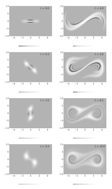
FIG. 3.: Stroboscopic phase space for the evolution in Fig.2-a. Horizontal axis corresponds to $x$, vertical axis to $p$. The medium grey shade on the background corresponds to zero values for the Wigner function, lighter and darker shades respectively to positive and negative values of $W(x,p)$

The four plots in the left column correspond to the decoherence period before the quench. The two Gaussian peaks (light spots) rotate in phase space around the minimum of the potential while the negative components (dark patches) of the Wigner function are cleared away by the environment. When the potential changes (right column) the wave packets start spreading and exploring the new non-linear regions of phase space giving rise to the dark interference patches. For longer times decoherence takes over again and the Wigner function becomes once more positively defined.

IV Single initial Gaussian state

As a further example we take a single Gaussian state centred at the global minimum of the quartic potential as initial condition. This is a more reasonable initial condition in terms of a realistic phase-transition, mimicking a high-temperature thermal distribution. It will also allow us to see that the above results are not an artifact of the initial state. This initial Wigner function is already classical and so we ignore the initial evolution period and take $t_{\rm c}=0$. Fig.4 and Fig.5 show the $\Gamma$ function for the same quenches as before (without and with temperature change respectively). The initial classical configuration ($\Gamma=0.$ for the initial time) develops quantum effects as the classical potential and the temperature change. The relevant time scales are evaluated as before and once again, the estimates are in good agreement with the simulation results. In the constant temperature case $\sigma_{p}(t_{\rm c}=0)\sim 0.7$ which gives $t_{\chi}\sim 0.6$ (see Fig.4). We also have $\sigma_{p}(t_{\rm max})\sim 3.2.$ and $\sigma_{\rm c}\sim 0.5$ leading to $t_{\rm D}\sim 3.2$, which agrees with the numerical result.

FIG. 4.: Evolution of $\Gamma$ when the potential changes its frequency from $\Omega_{0}^{2}=1\rightarrow-1$ for one Gaussian initially centred at $x=0$. ($\lambda=0.1$).

Fig.5 shows the cases where the change in frequency is followed by a change in the environmental temperature (same coefficients as in the example of Fig.2). For Fig.5-a $\sigma_{p}(t_{\rm max})\sim 3.3$ and $\sigma_{\rm c}=0.3$, and therefore the decoherence time is $t_{\rm D}\sim 3.5$. This scale is in good agreement with the numerical result. The estimation for Fig.5-b gives a decoherence time $t_{\rm D}\sim 4.5$ which again (as in the case of Fig.2-b) fails to fit the numerical result. We have included it in our analysis in order to emphasise how dramatic the quantum effects are during the quenched transition.

FIG. 5.: Evolution of $\Gamma$ when the potential changes its frequency from $\Omega_{0}^{2}=1\rightarrow-1$ for one Gaussian initially centred at $x=0$. ($\lambda=0.1$). A changing in the environment temperature is considered $D=0.3\rightarrow 0.1$ in (a) and $D=0.3\rightarrow 0.003$ in (b).

V Linear entropy

One of the most salient features of the quantum to classical transition concerns the production of entropy as a consequence of the entangling interactions between the system and the environment. In order to clarify the nature of the post-decoherence quantum effects in the systems simulated above we have looked at the corresponding time evolution of the linear entropy. This is given in terms of the density matrix by [4]:

$$S_{l}(t)=-\ln[{\mbox{Tr}}[\rho^{2}(t)]].$$ (16)

This quantity can be easily obtained from the Wigner function giving a good measurement of the ‘loss of purity’ of the system as it interacts with the bath (see [2, 4]). We found that as expected the entropy increases throughout the whole evolution. The system starts as a pure state and while interacting with the heat bath it looses coherence and simultaneously starts behaving as a classical ensemble. When the potential changes it evolves for some time as a quantum mixed system but the original ‘purity’ is never recovered. In this sense the decoherence process is irreversible. In terms of the Wigner function the linear entropy is related to the area of its non-zero component in phase space. Due to the coupling to the environment the total area is not conserved, the Wigner function keeps spreading at all times leading to permanent growth of the entropy.

Fig.6 shows the time dependent linear entropy (top plot) and its production rate (bottom plot) for the two different initial conditions considered before, in a quench with fixed environment temperature.

FIG. 6.: In the top figure, we show the linear entropy for the de-localised (solid line) and single Gaussian (dashed line) initial states. In the bottom figure, we have the entropy production rate vs time for the same initial conditions (solid and dashed lines as above).

In the case of the double-gaussian initial state (solid line) there is an initial period of evolution up to the first decoherence time $t_{D_{1}}=0.2$, where the linear entropy grows as a consequence of diffusion effects (as during the whole evolution) and also due to the disapearence of initial interference terms which are washed away by the environment. As these vanish the entropy production rate decreases as can be seen in the bottom plot. After an oscillation in the rate caused by the rotation of the Wigner function in the phase space which generates some low amplitude interference terms, the rate reaches a minimal value near the quench time at $t=t_{\rm c}$. After $t_{\rm c}$, the entropy rate starts growing again as the system gets rid of the newly induced interference terms. Finally at $t_{D_{2}}$, the entropy rate decreases to a low, slow decaying value driven by diffusion only.

The single gaussian evolution (dashed line) confirms this picture. From a low initial value (the initial state is free from negative terms) the entropy production rate grows as the quench generates interferences. Later, the environment cleans them out leading to the final decaying rate.

We should stress that a growing linear entropy function does not imply classicality (positivity of the Wigner function is an extra necessary condition in order to have a classical probability distribution). Increase of $S_{l}$ tells us that the pure initial quantum state is evolving into a mixed state. It does not of course, tell us whether this mixed state is a classical or quantum one. In particular this is the case between the quench time and the second decoherence time. During this period quantum effects are re-introduced while the linear entropy is still growing (faster even since its production rate increases).

VI Final remarks

We have shown, using an exact numerical evaluation of the Wigner function that quantum effects can be re-introduced after decoherence in several systems with explicit time dependence. These quantum effects are originated when the changing dynamics introduce instabilities in previously stable regions of the phase space. When this happens the dynamics of the Wigner function becomes more relevant than the decoherence effects due to the environment (and the lowest the final bath temperature the more dominant these are). The system then displays quantum behaviour for a length of time until the environment manages to catch up and force classicalization once again.

Since all examples so far were based on systems described by a double well potential one could wonder whether our results could be a consequence of possible tunnelling phenomena between the two minima. Tunnelling is possible between symmetry related eigenstates with energy below the barrier. The tunnelling time-scale for each pair is well known to be inversely proportional to the energy splitting of the symmetry related pair of eigenstates. For the parameters of our system ($\Omega^{2}=1$, $\lambda=0.1$, $\hbar=1$) only seven pairs of states are found below the barrier. Their energy splittings range from $\Delta E_{0}\sim 10^{-12}$ to $\Delta E_{7}\sim 10^{-2}$, and thus the tunnelling would firstly be expected after $t\sim 100$. Therefore and considering the time scales in which our simulations take place, tunnelling should play no role. The stretching and folding of the Wigner function responsible for the observed effects happens on both ‘sides’ of the potential well independently. This is in agreement with the conclusion invariably found in the literature (see for example Ref.[10]) that tunnelling takes place rather slowly when compared with all natural time-scales in the system.

In order to confirm directly that tunnelling phenomena are not responsible for the effects observed, we solved numerically the problem of a single Gaussian packet cantered at $x_{0}=2$ evolving in the usual quartic potential but with its motion restricted to $x>0$. The resulting $\Gamma$ is shown in Fig.7. As before quantum behaviour is swiftly recovered, the corresponding time scales being in good agreement with the analytical estimates.

FIG. 7.: Evolution for a single Gaussian packet cantered at $x_{0}=2$ ($t=0$) in a $x>0$ single-welled potential (and an infinite wall at $x=0$). We found $t_{\chi}=0.8$ and $t_{D}=7.4$ ($\Omega_{0}^{2}=-1$ and $D=0.01$).

Our results open up several interesting possibilities. The most obvious one would be to try to ‘maximise’ the recovering of quantum effects to the extent of making them effectively permanent. An oscillatory frequency [11] that would continuously force instabilities into the system could prevent classicalization or at least postpone it for a great length of time.

In terms of the specific case of the dynamics of a second-order phase transition one could expect quantum effects to be present. Though the model used is a crude simplification of what happens in a realistic phase transition, the same features of time-dependent introduction of non-linearities would be present in that case, leading to similar, probably stronger quantum effects. Critical properties of infinite dimensional systems such as critical slowing down could play an interesting role in the process.

- [1] C. Monroe et al., Science 272, 1131 (1996); C. J. Myatt, et al., Nature 403, 269 (2000); M. Brune et al., Phys. Rev. Lett. 77, 4887 (1996); A. Rauschenbeutel et al., Science 288, 2024 (2000); J. R. Friedman et al., Nature 406, 43 (2000); C. H. van del Wal et al., Science 290, 773, (2000); C. Tesche, Science 290, 720 (2000).
- [2] J. P. Paz and W. H. Zurek, Environment induced superselection and the transition from quantum to classical in Coherent matter waves, Les Houches Session LXXII, edited by R. Kaiser, C. Westbrook and F. David, EDP Sciences, Springer Verlag (Berlin) (2001) 533-614.
- [3] T. Bhattacharya, S. Habib, and K. Jacobs, Phys. Rev. Lett. 85, 4852 (2000) and references therein.
- [4] D. Monteoliva and J. P. Paz, Phys. Rev. Lett, 85, 3375 (2000); quant-ph/0106090.
- [5] B. L. Hu, J. P. Paz and Y. Zhang, Phys. Rev. D 47, 1576 (1993).
- [6] J. P. Paz, S. Habib, and W. H. Zurek, Phys. Rev. D47, 488 (1993).
- [7] F. C. Lombardo, F. D. Mazzitelli, and D. Monteoliva, Phys. Rev. D 62, 045016 (2000); F. C. Lombardo, F. D. Mazzitelli, and R. J. Rivers, hep-ph/0102152.
- [8] S. Habib, K. Jacobs, H. Mabuchi, R. Ryne, K. Shizume, and B. Sundaram, quant-ph/0010093.
- [9] W. H. Zurek and J. P. Paz, Phys. Rev. Lett. 72, 2508 (1994).
- [10] W.A. Lin and L.E.Ballentine, Phys. Rev. A45, 3637 (1992); R.Uttermann, T.Dittrich and P.Haenggi, Phys.Rev. E49, 273 (1994) ; T.Dittrich, B.Oelschlaegel and P.Haenggi, Europhys. Lett. 22, 5 (1993); S Kohler, R Utermann, P. Haenggi, et al. Phys.Rev. E58, 7219 (1998).
- [11] N. D. Antunes, F. C. Lombardo, and D. Monteoliva, in preparation.