Entanglement in the Quantum Heisenberg $XY$ model

Abstract

We study the entanglement in the quantum Heisenberg $XY$ model in which the so-called $W$ entangled states can be generated for 3 or 4 qubits. By the concept of concurrence, we study the entanglement in the time evolution of the $XY$ model. We investigate the thermal entanglement in the two-qubit isotropic $XY$ model with a magnetic field and in the anisotropic $XY$ model, and find that the thermal entanglement exists for both ferromagnetic and antiferromagnetic cases. Some evidences of the quantum phase transition also appear in these simple models.

]

I Introduction

Quantum entanglement has been studied intensely in recent years due to its potential applications in quantum communication and information processing[1] such as quantum teleportation[2], superdense coding[3], quantum key distribution[4], and telecoloning[5]. Recently Dür et al.[6] found that truly tripartite pure state entanglement of three qubits is either equivalent to the maximally entangled GHZ state[7] or to the so-called $W$ state[6]

$$|W\rangle=\frac{1}{\sqrt{3}}(|100\rangle+|010\rangle+|001\rangle).$$ (1)

For the GHZ state, if one of the three qubits is traced out, the remaining state is unentangled, which means that this state is fragile under particle losses. Oppositely the entanglement of $W$ state is maximally robust under disposal of any one of the three qubits [6].

A natural generalization of the $W$ state to $N$ qubits and arbitrary phases is

$$|W_{N}\rangle = \frac{1}{\sqrt{N}}(e^{i\theta_{1}}|1000...0\rangle+e^{i\theta_{2}}|0100...0\rangle+$$ (3)

$$e^{i\theta_{3}}|0010...0\rangle+\cdot\cdot\cdot+e^{i\theta_{N}}|0000...1\rangle).$$

For the above state $|W_{N}\rangle$, the concurrences [6, 8] between any two qubits are all equal to $2/N$ and do not depend on the phases $\theta_{i}(i=1,2...N)$. This shows that any two qubits in the $W$ state are equally entangled. Recently Koashi et al.[9] shows that the maximum degree of entanglement (measured in the concurrence) between any pair of qubits of a $N$-qubit symmetric state is $2/N$. This tight bound is achieved when the qubits are prepared in the state $|W_{N}\rangle$.

The Heisenberg interaction has been used to implement quantum computer[10]. It can be realized in quantum dots[10], nuclear spins[11], electronic spins[12] and optical lattices[13]. By suitable coding, the Heisenberg interaction alone can be used for quantum computation[14].

Here we consider the quantum Heisenberg $XY$ model, which was intensively investigated in 1960 by Lieb, Schultz, and Mattis[15]. Recently Imamoḡlu et al have studied the quantum information processing using quantum dot spins and cativity QED[16] and obtained an effective interaction Hamiltonian between two quantum dots, which is just the $XY$ Hamiltonian. The effective Hamiltonian can be used to construct the controlled-NOT gate[16]. The $XY$ model is also realized in the quantum-Hall system[17] and in cavity QED system[18] for a quantum computer.

The $XY$ Hamiltonian is given by[15]

$$H=J\sum_{n=1}^{N}\left(S_{n}^{x}S_{n+1}^{x}+S_{n}^{y}S_{n+1}^{y}\right),$$ (4)

where $S^{\alpha}=\sigma^{\alpha}/2$ $(\alpha=x,y,z)$ are spin 1/2 operators, $\sigma^{\alpha}$ are Pauli operators, and $J>0$ is the antiferromagnetic exchange interaction between spins. We adopt the periodic boundary condition, i.e., $S_{N+1}^{x}=S_{1}^{x},$ $S_{N+1}^{y}=S_{1}^{y}.$

One role of the $XY$ model in quantum computation is that it can be used to construct the swap gate. The evolution operator of the corresponding two-qubit $XY$ model is given by

$$U(t)=\exp\left[-iJt(\sigma_{1}^{x}\sigma_{2}^{x}+\sigma_{1}^{y}\sigma_{2}^{y})/2\right].$$ (5)

Choosing $Jt=\pi/2,$ we have

$\displaystyle U\left(\frac{\pi}{2J}\right)|00\rangle=|00\rangle,\text{ }U\left(\frac{\pi}{2J}\right)|11\rangle=|11\rangle,$

$$U\left(\frac{\pi}{2J}\right)|01\rangle=-i|10\rangle,\text{ }U\left(\frac{\pi}{2J}\right)|10\rangle=-i|01\rangle.$$ (6)

The above equation shows that the operator $U\left(\frac{\pi}{2J}\right)$ acts as a swap gate up to a phase. Another gate $\sqrt{\text{swap}}$ which is universal can also be constructed simply as $U\left(\frac{\pi}{4J}\right).$ A swap gate can be realized by successive three C-NOT gates[19], while here we only need one-time evolution of the $XY$ model. This shows that the $XY$ model has some potential applications in quantum computation.

The entanglement in the ground state of the Heisenberg model has been discussed by O’Connor and Wootters[20]. Here we study the entanglement in the $XY$ model. We first consider the generation of $W$ states in the $XY$ model. It is found that for 3 and 4 qubits, the $W$ states can be generated at certain times. By the concept of concurrence, we study the entanglement properties in the time evolution of the $XY$ model. Finally we discuss the thermal entanglement in the two-qubit $XY$ model with a magnetic field and in the anisotropic $XY$ model.

II Solution of the $XY$ model

With the help of raising and lowering operators $\sigma_{n}^{\pm}=S_{n}^{x}\pm iS_{n}^{y},$ the Hamiltonian $H$ is rewritten as ($J=1)$

$$H={1\over 2}\sum_{n=1}^{N}\left(\sigma_{n}^{+}\sigma_{n+1}^{-}+\sigma_{n+1}^{+}\sigma_{n}^{-}\right).$$ (7)

Obviously the states with all spins down $|0\rangle^{\otimes N}$ or all spins up $|1\rangle^{\otimes N}$ are eigenstates with zero eigenvalues.

The eigenvalue problem of the $XY$ model can be exactly solved by the Jordan-Wigner transformation[21]. Here we are only interested in the time evolution problem and in the ‘one particle’ states ($N-1$ spins down, one spin up),

$$|k\rangle=\sum_{n=1}^{N}a_{k,n}\sigma_{n}^{+}|0\rangle^{\otimes N}.$$ (8)

The eigenequation is given by

$$H|\Psi\rangle = \frac{1}{2}\sum_{n=1}^{N}(a_{k,n+1}+a_{k,n-1})\sigma_{n}^{+}|0\rangle^{\otimes N}$$ (9)

$$= E_{k}\sum_{n=1}^{N}a_{k,n}\sigma_{n}^{+}|0\rangle^{\otimes N}.$$ (10)

Then the coefficients $a_{k,n}$ satisfy

$$\frac{1}{2}(a_{k,n+1}+a_{k,n-1})=E_{k}a_{k,n}.$$ (11)

The solution of the above equation is

$$a_{k,n} = \exp\left(\frac{i2\pi nk}{N}\right)(k=1...N),$$ (12)

$$E_{k} = \cos\left(\frac{2\pi k}{N}\right),$$ (13)

where we have used the periodic boundary condition.

So the eigenvectors are given by

$$|k\rangle=\frac{1}{\sqrt{N}}\sum_{n=1}^{N}\exp\left(\frac{i2\pi nk}{N}\right)\sigma_{n}^{+}|0\rangle^{\otimes N}$$ (14)

which satisfy $\langle k|k^{\prime}\rangle=\delta_{kk^{\prime}}.\,$It is interesting to see that all the eigenstates are generalized $W$ states (Eq.(3)).

Note that the $XY$ Hamiltonian $H$ commutes with the operator

$$Q=\sigma_{x}^{\otimes N}=\sigma_{x}\otimes\sigma_{x}\otimes...\otimes\sigma_{x},$$ (15)

then the state

$$|k\rangle^{\prime}=\frac{1}{\sqrt{N}}\sum_{n=1}^{N}\exp\left(\frac{i2\pi nk}{N}\right)\sigma_{n}^{-}|1\rangle^{\otimes N}$$ (16)

are also the eigenstates of $H$ with eigenvalues $\cos\left(2\pi k/N\right).$

Now we choose the initial state of the system as $\sigma_{1}^{+}|0\rangle^{\otimes N},\,$and in terms of the eigenstates $|k\rangle$, it can be expressed as

$$|\Psi(0)\rangle=\frac{1}{\sqrt{N}}\sum_{k=1}^{N}\exp\left(\frac{-i2\pi k}{N}\right)|k\rangle.$$ (17)

The state vector at time $t$ is easily obtained as

$$|\Psi(t)\rangle=\sum_{n=1}^{N}b_{n}(t)\sigma_{n}^{+}|0\rangle^{\otimes N},$$ (18)

where

$$b_{n}(t)=\frac{1}{N}\sum_{k=1}^{N}e^{i2\pi(n-1)k/N-it\cos\left(2\pi k/N\right).}$$ (19)

If we choose the initial state as $\sigma_{1}^{-}|1\rangle^{\otimes N},$ then the wave vector at time $t$ will be $\sum_{n=1}^{N}b_{n}(t)\sigma_{n}^{-}|1\rangle^{\otimes N}.$

III Generation of $W$ states

From Eq.(18), the probabilities at time $t$ for state $\sigma_{n}^{+}|0\rangle^{\otimes N}$ is obtained as

$$P(n,N,t)=|b_{n}(t)|^{2}.$$ (20)

For $N=2$, it is easy to see that the probability $P(1,2,t)=\cos^{2}t$ , $P(2,2,t)=\sin^{2}t.\,$The state vector at time $t$ is

$$|\Psi(t)\rangle=\cos t|10\rangle-i\sin t|01\rangle.$$ (21)

When $t=\pi/4,$ the above state is the maximally entangled state.

Now we consider the case $N=3.$ The probabilities are analytically obtained as

$$P(1,3,t) = \frac{1}{9}\left[5+4\cos\left(\frac{3}{2}t\right)\right],$$ (22)

$$P(2,3,t) = P(3,3,t)=\frac{1}{9}\left[2-2\cos\left(\frac{3}{2}t\right)\right].$$ (23)

Fig.1(a) gives a plot of the probabilities versus time. It is clear that there exist some cross points of the probabilities. At these special times the probabilities $P(n,3,t)$ are all equal to 1/3, which indicates the $W$ states are generated. From Eq.(23), we see that if the time $t$ satisfies the equation

$$\cos\left(\frac{3}{2}t\right)=-\frac{1}{2},$$ (24)

the probabilities are same. The solution of Eq.(24) is

$$t_{n} = \frac{4\pi}{9}+\frac{4n\pi}{3},$$ (25)

$$t_{n}^{\prime} = \frac{8\pi}{9}+\frac{4n\pi}{3}(n=0,1,2,...).$$ (26)

Explicitly at these time points, the corresponding state vectors are

$$|\Psi(t_{n})\rangle = \frac{1}{\sqrt{3}}\left(|100\rangle+e^{\frac{-i2\pi}{3}}|010\rangle+e^{\frac{-i2\pi}{3}}|001\rangle\right),$$ (27)

$$|\Psi(t_{n}^{\prime})\rangle = \frac{1}{\sqrt{3}}\left(|100\rangle+e^{\frac{i2\pi}{3}}|010\rangle+e^{\frac{i2\pi}{3}}|001\rangle\right)$$ (28)

which are the generalized $W$ state for $N=3.$

FIG. 1.: Time evolution of the probabilities and concurrences for $N=3$. (a)The probablity plus 1 for $n=1$ (solid line) and $n=2,n=3$ (dotted line); (b)The concurrences $C_{12}(t),C_{13}(t)$(solid line) and $C_{23}(t)$ (dotted line).

For the case $N=4,$ the probabilities are given by

$$P(1,4,t) = \cos^{4}\left(\frac{t}{2}\right),\text{ }P(3,4,t)=\sin^{4}\left(\frac{t}{2}\right),$$ (29)

$$P(2,4,t) = P(4,4,t)=\frac{1}{4}\sin^{2}t,$$ (30)

As seen from Fig.2(a), there also exists some cross points, which indicates the 4-qubit $W$ states are generated. The probabilities are same when

$$t_{n} = \frac{\pi}{2}+2n\pi,$$ (31)

$$t_{n}^{\prime} = \frac{3\pi}{2}+2n\pi(n=0,1,2,...)$$ (32)

Explicitly the 4-qubit $W$ states are

$$|\Psi(t_{n})\rangle = \frac{1}{2}\left(|1000\rangle-i|0100\rangle-|0010\rangle-i|0001\rangle\right),$$ (33)

$$|\Psi(t_{n}^{\prime})\rangle = \frac{1}{2}\left(|1000\rangle+i|0100\rangle-|0010\rangle+i|0001\rangle\right).$$ (34)

FIG. 2.: Time evolution of the probabilities and concurrences for $N=4$. (a)The probablity plus 1 for $n=1$ (solid line), $n=3$ (dotted line) and $n=2,n=4$ (dashed line); (b)The concurrences $C_{12}(t)$ (solid line) and $C_{23}(t)$(dotted line).

Can we generate $W$ states for more than 4 qubits in the $XY$ model? Fig.3(a) shows that there is no cross points for $N=5$ . Further numerical calculations for long time and large $N$ show no evidence that there exist some times at which the $W$ states can be generated.

FIG. 3.: Time evolution of the probabilities and concurrences for $N=5$. (a)The probablity plus 1 for $n=1$ (solid line), $n=3,n=4$ (dotted line) and $n=2,n=5$ (dashed line);(b)The concurrences $C_{12}(t)$ (solid line) and $C_{23}(t)$(dotted line).

We see that the $W$ states appear periodically for 3 and 4 qubits. In order that a certain state occurs periodically in a system, a necessary condition is that the ratio of any two frequencies available in the system is a rational number. From Eq.(13) it is easy to check that the necessary condition is satisfied for 2, 3, 4, and 6 qubits. For 6 qubits the corresponding probabilities evolve periodically with time. The numerical calculations show that there exists no cross points, i.e., we can not creat 6-qubit $W$ state. However some states close to the $W$ state will occur repeatedly and these states may be used for quantum computation.

The 3-qubit and 4-qubit $W$ states are readily generated by only one-time evolution of the $XY$ system. This idea is similar to the concurrent quantum computation[22] in which some functions of computation are realized by only one-time evolution of multi-qubit interaction systems.

The $W$ entangled states can be generated by other methods, such as coupling $N$ spins with a quantized electromagnetic field. However here we only use the interaction of $N$ spins themselves and do not need to introduce additional degree of freedoms.

IV Time evolution of entanglement

We first briefly review the definition of concurrence[8]. Let $\rho_{12}$ be the density matrix of a pair of qubits $1$ and $2.$ The density matrix can be either pure or mixed. The concurrence corresponding to the density matrix is defined as

$$C_{12}=\max\left\{\lambda_{1}-\lambda_{2}-\lambda_{3}-\lambda_{4},0\right\}$$ (36)

where the quantities $\lambda_{1}\geq\lambda_{2}\geq\lambda_{3}\geq$ $\lambda_{4}$ are the square roots of the eigenvalues of the operator

$$\varrho_{12}=\rho_{12}(\sigma_{y}\otimes\sigma_{y})\rho_{12}^{*}(\sigma_{y}\otimes\sigma_{y}).$$ (37)

The nonzero concurrence implies that the qubits 1 and 2 are entangled. The concurrence $C_{12}=0$ corresponds to an unentangled state and $C_{12}=1$ corresponds to a maximally entangled state.

We consider the entanglement in the state $|\Psi(t)\rangle$(18). By direct calculations, the concurrence between any two qubits $i$ and $j$ are simply obtained as

$$C_{ij}(t)=2|b_{i}(t)b_{j}(t)|.$$ (38)

The numerical results for the concurrence are shown in Fig.1(b), Fig.2(b) and Fig.3(b).

For $N=3,$ Fig.1(b) shows that the entanglement is periodic with period $4\pi/3.$ At times $4n\pi/3(n=1,2,3,...)$, the state vectors are disentangled and become the state $|100\rangle$ up to a phase. The concurrences of $C_{12}(t)$ and $C_{13}(t)$ are same, and have two maximum points in one period, while the concurrence $C_{13}(t)$ has only one maximum point. Fig.2(b) shows the concurrences for $N=4.$ They are periodic with period $2\pi.$ In one period there are two unentanglement points, $t=\pi,2\pi.$ For both concurrences $C_{12}(t)$ and $C_{23}(t)$, there are two maximum points in one period. If we choose large $N$ (see Fig.3(b) for $N=5$), there exists no exact periodicity for the entanglements of two qubits. From the time evolution of the concurrences we can see clearly when the system becomes disentangled and when the system maximally entangled.

V Thermal entanglement

Recently the concept of thermal entanglement was introduced and studied within one-dimensional isotropic Heisenberg model[23]. Here we study this kind of entanglement within both the isotropic $XY$ model with a magnetic field and the anisotropic $XY$ model.

A Isotropic $XY$ model with a magnetic field

We consider the two-qubit isotropic antiferromagnetic $XY$ model in a constant external magnetic field $B,$

$$H=\frac{B}{2}(\sigma_{1}^{z}+\sigma_{2}^{z})+J\left(\sigma_{1}^{+}\sigma_{2}^{-}+\sigma_{2}^{+}\sigma_{1}^{-}\right).$$ (39)

The eigenvalues and eigenvectors of $H$ are easily obtained as

$$H|00\rangle = -B|00\rangle,H|11\rangle=B|11\rangle,$$ (40)

$$H|\Psi^{\pm}\rangle = \pm J|\Psi^{\pm}\rangle,$$ (41)

where $|\Psi^{\pm}\rangle=\frac{1}{\sqrt{2}}(|01\rangle\pm|10\rangle)$ are maximally entangled states.

The state of the system at thermal equilibrium is $\rho(T)=\exp\left(-\frac{H}{kT}\right)/Z,$ where $Z=$Tr$\left[\exp\left(-\frac{H}{kT}\right)\right]$ is the partition function and $k$ is the Boltzmann’s constant. As $\rho(T)$ represents a thermal state, the entanglement in the state is called thermal entanglement[23].

In the standard basis, $\left\{|00\rangle,|01\rangle,|10\rangle,|11\rangle\right\},$ the density matrix $\rho(T)$ is written as ($k=1$)

$$\rho(T) = \frac{1}{2(\cosh\frac{J}{T}+\cosh\frac{B}{T})}$$ (47)

$$\times\left(\begin{array}[]{llll}e^{-\frac{B}{T}}&0&0&0\\ 0&\cosh\frac{J}{T}&-\sinh\frac{J}{T}&0\\ 0&-\sinh\frac{J}{T}&\cosh\frac{J}{T}&0\\ 0&0&0&e^{\frac{B}{T}}\end{array}\right)$$

From Eqs.(36),(37) and (47), the concurrence is given by

$$C=\max\left(\frac{\sinh\frac{J}{T}-1}{\cosh\frac{J}{T}+\cosh\frac{B}{T}},0\right).$$ (48)

Then we know $C=0$ if $\sinh\frac{J}{T}\leq 1,\,$i.e., there is a critical temperature

$$T_{c}=\frac{J}{\arcsin\text{h}(1)}\approx 1.1346J,$$ (49)

the entanglement vanishes for $T\geq T_{c}.$ It is interesting to see that the critical temperature is independent on the magnetic field $B.$

For $B=0,$ the maximally entangled state $|\Psi^{-}\rangle$ is the ground state with eigenvalue $-J.$ Then the maximum entanglement is at $T=0,$ i.e., $C=1.\,$As $T$ increases, the concurrence decreases as seen from Fig.4 due to the mixing of other states with the maximally entangled state. For a high value of $B$ (say $B=1.2$), the state $|00\rangle\,$becomes the ground state, which means there is no entanglement at $T=0.$ However by increasing $T,$ the maximally entangled states $|\Psi^{\pm}\rangle$ will mix with the state $|00\rangle,$ which makes the entanglement increase (see Fig.4).

FIG. 4.: The concurrences versus temperature for different magnetic fields. The parameter $J$ is set to one.

From Fig.5 we see that there is a evidence of phase transition for small temperature by increasing magnetic field. Now we do the limit $T\rightarrow 0\,$on the concurrence (48), we obtain

$$\lim_{T\rightarrow 0}C = 1\text{ for }B<J,$$ (50)

$$\lim_{T\rightarrow 0}C = \frac{1}{2}\text{ for }B=J,$$ (51)

$$\lim_{T\rightarrow 0}C = 0\text{ for }B>J.$$ (52)

So we can see that at $T=0,$ the entanglement vanishes as $B$ crosses the critical value $J.$ This is easily understand since we see that if $B>J,$ the ground state will be the unentangled state $|00\rangle.$ This special point $T=0,B=J,$ at which entanglement becomes a nonanalytic function of $B,$ is the point of quantum phase transition[24].

FIG. 5.: The concurrences versus magnetic field B for different temperatures. The parameter $J$ is set to one.

It should be pointed out that the results of thermal entanglement in the present isotropic $XY$ model is qualitatively the same as but quantitatively different from that in the isotropic Heisenberg model[23]. An important conclusion is that the concurrences are the same for both positive $J$ and negative $J$ in the $XY$ model. That is to say, the entanglement exists for both antiferromagnetic and ferromagnetic cases. In contrary to this, for the case of two-qubit Heisenberg model, no thermal entanglement exists for the ferromagnetic case.

B Anisotropic $XY$ model

Now we consider the two-qubit anisotropic antiferromagnetic $XY$ model which is described by the Hamiltonian[15]

$$H_{a} = \frac{J}{2}\left[(1+\gamma)\sigma_{1}^{x}\sigma_{2}^{x}+(1-\gamma)\sigma_{1}^{y}\sigma_{2}^{y}\right],$$ (53)

$$= J\left(\sigma_{1}^{+}\sigma_{2}^{-}+\sigma_{2}^{+}\sigma_{1}^{-}\right)+J\gamma\left(\sigma_{1}^{+}\sigma_{2}^{+}+\sigma_{2}^{-}\sigma_{1}^{-}\right).$$ (54)

where $\gamma$ is the anisotropic parameter. Obviously the eigenvalues and eigenvectors of the Hamiltonian $H_{a}$ is given by $H_{a}|\Psi^{\pm}\rangle=\pm J|\Psi^{\pm}\rangle$ and $H_{a}|\Phi^{\pm}\rangle=\pm J\gamma|\Phi^{\pm}\rangle,$ where $|\Phi^{\pm}\rangle=\frac{1}{\sqrt{2}}(|00\rangle\pm|11\rangle).$ Then the four maximally entangled Bell states are the eigenstates of the Hamiltonian $H_{a}.$ Although the anisotropic parameter can be arbitrary, we restrict ourselves on $0\leq\gamma\leq 1.$ The parameter $\gamma=0$ and 1 correspond to the isotropic $XY$ model and Ising model respectively. Thus the anisotropic $XY$ model can be considered as a interpolating Hamiltonian between the isotropic $XY$ model and the Ising model. The anisotropic parameter $\gamma$ controls the interpolation.

The density matrix $\rho(T)$ in the standard basis is given by

$\rho(T)=\frac{1}{2(\cosh\frac{J}{T}+\cosh\frac{J\gamma}{T})}$

$\times\left(\begin{array}[]{llll}\cosh\frac{J\gamma}{T}&0&0&-\sinh\frac{J\gamma}{T}\\ 0&\cosh\frac{J}{T}&-\sinh\frac{J}{T}&0\\ 0&-\sinh\frac{J}{T}&\cosh\frac{J}{T}&0\\ -\sinh\frac{J\gamma}{T}&0&0&\cosh\frac{J\gamma}{T}\end{array}\right)$

(55)

The square root of the eigenvalues of the operator $\varrho_{12}$ are $\frac{e^{\pm J/T}}{2(\cosh\frac{J}{T}+\cosh\frac{J\gamma}{T})}$ and $\frac{e^{\pm J\gamma/T}}{2(\cosh\frac{J}{T}+\cosh\frac{J\gamma}{T})}.\,$ Then from Eq.(36), the concurrence is given by

$$C=\max\left(\frac{\sinh\frac{J}{T}-\cosh\frac{J\gamma}{T}}{\cosh\frac{J}{T}+\cosh\frac{J\gamma}{T}},0\right)$$ (56)

As we expected Eq. (56) reduces to Eq. (48) with $B=0$ when $\gamma=0.$ When $\gamma=1,$ the concurrence $C=0,$ which indicates that no thermal entanglement appears in the two-qubit Ising model. In this anisotropic model, the concurrences are the same for both positive $J$ and negative $J$ , i.e, the thermal entanglement is the same for the antiferromagnetic and ferromagnetic cases. The critical temperature $T_{c\text{ }}$is determined by the nonlinear equation

$\displaystyle\sinh\frac{J}{T}=\cosh\frac{J\gamma}{T},$

which can be solved numerically.

In Fig.6 we give a plot of the concurrence as a function of temperature $T$ for different anisotropic parameters. At zero temperature the concurrence is 1 since no matter what the sign of $J$ is and what the values of $\gamma$ are, the ground state is one of the Bell states, the maximally entangled state. The concurrence monotonically decreases with the increase of temperature until it reaches the critical value of $T$ and becomes zero. The numerical calculations also show that the critical temperature decreases as the anisotropic parameter increases from 0 to 1.

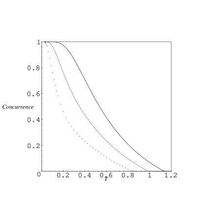
FIG. 6.: The concurrences versus temperature for different aniosotropic parameters: $\gamma=0$ (solid line), $\gamma=0.6$ (dashed line) and $\gamma=0.8$ (dotted line). The parameter $J$ is set to one.

VI Conclusions

In conclusion, we have presented some interesting results in the simple $XY$ model. First, we can use $XY$ interaction to generate the 3-qubit and 4-qubit $W$ entangled states. Second, we see that the time evolution of entanglement are periodic for 2, 3, 4 and 6 qubits, and there is no exact periodicity for large $N$. At some special points the states becomes disentangled. Finally we study the thermal entanglement within a two-qubit isotropic $XY$ model with a magnetic field and an anisotropic $XY$ model, and find that the thermal entanglement exists for both ferromagnetic and antiferromagnetic cases. Even in the simple model we see some evidence of the quantum phase transition.

The entanglement is not completely determined by the partition function, i.e., by the usual quantum statistical physics. It is a good challenge to study the entanglement in multi-qubit quantum spin models.

- [1] Special issue on quantum information, Phys. World, 11, 33-57 (1998).
- [2] C. H. Bennett et al. Phys. Rev. Lett. 70, 1895 (1993).
- [3] C. H. Bennett and S. J. Wiesner, Phys. Rev. Lett. 69, 2881 (1992).
- [4] A. K. Ekert, Phys. Rev. Lett. 67, 661 (1991).
- [5] M. Murao et al. Phys. Rev. A 59, 156 (1999).
- [6] W. Dür, G. Vidal and J. I. Cirac, Phys. Rev. A 62, 062314 (2000).
- [7] D. M. Greenberger, M. Horne, A. Zeilinger, Bell’s theorem, Quantum Theory, and Conceptions of the Universe, ed. M. Kafatos, Kluwer, Dordrecht 69 (1989); D. Bouwmeester et al., Phys. Rev. Lett. 82 , 1345 (1999).
- [8] S. Hill and W. K. Wootters, Phys. Rev. Lett. 78, 5022 (1997); W. K. Wootters, Phys. Rev. Lett. 80, 2245; V. Coffman, J. Kundu, and W. K. Wootters, Phys. Rev. A61, 052306 (2000).
- [9] M. Koashi, V. Bužek, and N. Imoto, Phys. Rev. A 62, 050302 (2000).
- [10] D. Loss and D. P. Divincenzo, Phys. Rev. A57, 120 (1998); G. Burkard, D. Loss and D. P. DiVincenzo,Phys. Rev. B59, 2070 (1999).
- [11] B. E. Kane, Nature 393, 133 (1998).
- [12] R. Vrijen et al., quant-ph/9905096.
- [13] Anders Sørensen and Klaus Mølmer, Phys. Rev. Lett. 83, 2274 (1999).
- [14] D. A. Lidar, D. Bacon, and K. B. Whaley, Phys. Rev. Lett. 82, 4556 (1999); D. P. DiVincenzo, D. Bacon, J. Kempe, G. Burkard, and K. B. Whaley, Nature 408, 339 (2000)
- [15] E. Lieb, T. Schultz, and D. Mattis, Ann. Phys. (N. Y.) 16, 407 (1961).
- [16] A. Imamoḡlu, D. D. Awschalom, G. Burkard, D. P. DiVincenzo, D. Loss, M. Sherwin, and A. Small, Phys. Rev. Lett. 83, 4204 (1999).
- [17] V. Privman, I. D. Vagner and G. Kventsel, quant-ph/9707017.
- [18] S. B. Zheng, G. C. Guo, Phys. Rev. Lett. 85, 2392 (2000).
- [19] L. You, M. S. Chapman, Phys. Rev. A 62, 052302 (2000).
- [20] K. M. O’Connor, W. K. Wootters, quant-ph/0009041.
- [21] P. Jordan and E. Wigner, Z. Phys. 47, 631 (1928).
- [22] F. Yamaguchi, C. P. Master and Y. Yamamoto, quant-ph/0005128.
- [23] M. C. Arnesen, S. Bose, and V. Vedral, quant-ph/0009060; M. A. Nielsen, quant-ph/0011036.
- [24] S. Sachdev, Quantum phase transitions (Cambridge University Press, Cambridge, 1999).