Quantum Theory From Five Reasonable Axioms

Abstract

The usual formulation of quantum theory is based on rather obscure axioms (employing complex Hilbert spaces, Hermitean operators, and the trace formula for calculating probabilities). In this paper it is shown that quantum theory can be derived from five very reasonable axioms. The first four of these axioms are obviously consistent with both quantum theory and classical probability theory. Axiom 5 (which requires that there exist continuous reversible transformations between pure states) rules out classical probability theory. If Axiom 5 (or even just the word “continuous” from Axiom 5) is dropped then we obtain classical probability theory instead. This work provides some insight into the reasons why quantum theory is the way it is. For example, it explains the need for complex numbers and where the trace formula comes from. We also gain insight into the relationship between quantum theory and classical probability theory.

1 Introduction

Quantum theory, in its usual formulation, is very abstract. The basic elements are vectors in a complex Hilbert space. These determine measured probabilities by means of the well known trace formula - a formula which has no obvious origin. It is natural to ask why quantum theory is the way it is. Quantum theory is simply a new type of probability theory. Like classical probability theory it can be applied to a wide range of phenomena. However, the rules of classical probability theory can be determined by pure thought alone without any particular appeal to experiment (though, of course, to develop classical probability theory, we do employ some basic intuitions about the nature of the world). Is the same true of quantum theory? Put another way, could a 19th century theorist have developed quantum theory without access to the empirical data that later became available to his 20th century descendants? In this paper it will be shown that quantum theory follows from five very reasonable axioms which might well have been posited without any particular access to empirical data. We will not recover any specific form of the Hamiltonian from the axioms since that belongs to particular applications of quantum theory (for example - a set of interacting spins or the motion of a particle in one dimension). Rather we will recover the basic structure of quantum theory along with the most general type of quantum evolution possible. In addition we will only deal with the case where there are a finite or countably infinite number of distinguishable states corresponding to a finite or countably infinite dimensional Hilbert space. We will not deal with continuous dimensional Hilbert spaces.

The basic setting we will consider is one in which we have preparation devices, transformation devices, and measurement devices. Associated with each preparation will be a state defined in the following way:

The state

associated with a particular preparation is defined to be (that thing represented by) any mathematical object that can be used to determine the probability associated with the outcomes of any measurement that may be performed on a system prepared by the given preparation.

Hence, a list of all probabilities pertaining to all possible measurements that could be made would certainly represent the state. However, this would most likely over determine the state. Since most physical theories have some structure, a smaller set of probabilities pertaining to a set of carefully chosen measurements may be sufficient to determine the state. This is the case in classical probability theory and quantum theory. Central to the axioms are two integers $K$ and $N$ which characterize the type of system being considered.

• The number of degrees of freedom, $K$, is defined as the minimum number of probability measurements needed to determine the state, or, more roughly, as the number of real parameters required to specify the state.

• The dimension, $N$, is defined as the maximum number of states that can be reliably distinguished from one another in a single shot measurement.

We will only consider the case where the number of distinguishable states is finite or countably infinite. As will be shown below, classical probability theory has $K=N$ and quantum probability theory has $K=N^{2}$ (note we do not assume that states are normalized).

The five axioms for quantum theory (to be stated again, in context, later) are

Axiom 1

Probabilities. Relative frequencies (measured by taking the proportion of times a particular outcome is observed) tend to the same value (which we call the probability) for any case where a given measurement is performed on a ensemble of $n$ systems prepared by some given preparation in the limit as $n$ becomes infinite.

Axiom 2

Simplicity. $K$ is determined by a function of $N$ (i.e. $K=K(N)$) where $N=1,2,\dots$ and where, for each given $N$, $K$ takes the minimum value consistent with the axioms.

Axiom 3

Subspaces. A system whose state is constrained to belong to an $M$ dimensional subspace (i.e. have support on only $M$ of a set of $N$ possible distinguishable states) behaves like a system of dimension $M$.

Axiom 4

Composite systems. A composite system consisting of subsystems $A$ and $B$ satisfies $N=N_{A}N_{B}$ and $K=K_{A}K_{B}$

Axiom 5

Continuity. There exists a continuous reversible transformation on a system between any two pure states of that system.

The first four axioms are consistent with classical probability theory but the fifth is not (unless the word “continuous” is dropped). If the last axiom is dropped then, because of the simplicity axiom, we obtain classical probability theory (with $K=N$) instead of quantum theory (with $K=N^{2}$). It is very striking that we have here a set of axioms for quantum theory which have the property that if a single word is removed – namely the word “continuous” in Axiom 5 – then we obtain classical probability theory instead.

The basic idea of the proof is simple. First we show how the state can be described by a real vector, ${\bf p}$, whose entries are probabilities and that the probability associated with an arbitrary measurement is given by a linear function, ${\bf r}\cdot{\bf p}$, of this vector (the vector ${\bf r}$ is associated with the measurement). Then we show that we must have $K=N^{r}$ where $r$ is a positive integer and that it follows from the simplicity axiom that $r=2$ (the $r=1$ case being ruled out by Axiom 5). We consider the $N=2$, $K=4$ case and recover quantum theory for a two dimensional Hilbert space. The subspace axiom is then used to construct quantum theory for general $N$. We also obtain the most general evolution of the state consistent with the axioms and show that the state of a composite system can be represented by a positive operator on the tensor product of the Hilbert spaces of the subsystems. Finally, we show obtain the rules for updating the state after a measurement.

This paper is organized in the following way. First we will describe the type of situation we wish to consider (in which we have preparation devices, state transforming devices, and measurement devices). Then we will describe classical probability theory and quantum theory. In particular it will be shown how quantum theory can be put in a form similar to classical probability theory. After that we will forget both classical and quantum probability theory and show how they can be obtained from the axioms.

Various authors have set up axiomatic formulations of quantum theory, for example see references [1, 2, 3, 4, 5, 6, 7, 8, 9, 10] (see also [11, 12, 13]). Much of this work is in the quantum logic tradition. The advantage of the present work is that there are a small number of simple axioms, these axioms can easily be motivated without any particular appeal to experiment, and the mathematical methods required to obtain quantum theory from these axioms are very straightforward (essentially just linear algebra).

2 Setting the Scene

We will begin by describing the type of experimental situation we wish to consider (see Fig. 1). An experimentalist has three types of device. One is a preparation device. We can think of it as preparing physical systems in some state.

Figure 1: The situation considered consists of a preparation device with a knob for varying the state of the system produced and a release button for releasing the system, a transformation device for transforming the state (and a knob to vary this transformation), and a measuring apparatus for measuring the state (with a knob to vary what is measured) which outputs a classical number.

It has on it a number of knobs which can be varied to change the state prepared. The system is released by pressing a button. The system passes through the second device. This device can transform the state of the system. This device has knobs on it which can be adjusted to effect different transformations (we might think of these as controlling fields which effect the system). We can allow the system to pass through a number of devices of this type. Unless otherwise stated, we will assume the transformation devices are set to allow the system through unchanged. Finally, we have a measurement apparatus. This also has knobs on it which can be adjusted to determine what measurement is being made. This device outputs a classical number. If no system is incident on the device (i.e. because the button on the preparation device was not pressed) then it outputs a 0 (corresponding to a null outcome). If there is actually a physical system incident (i.e when the release button is pressed and the transforming device has not absorbed the system) then the device outputs a number $l$ where $l=1$ to $L$ (we will call these non-null outcomes). The number of possible classical outputs, $L$, may depend on what is being measured (the settings of the knobs).

The fact that we allow null events means that we will not impose the constraint that states are normalized. This turns out to be a useful convention. It may appear that requiring the existence of null events is an additional assumption. However, it follows from the subspace axiom that we can arrange to have a null outcome. We can associate the non-null outcomes with a certain subspace and the null outcome with the complement subspace. Then we can restrict ourselves to preparing only mixtures of states which are in the non-null subspace (when the button is pressed) with states which are in the null subspace (when the button is not pressed).

The situation described here is quite generic. Although we have described the set up as if the system were moving along one dimension, in fact the system could equally well be regarded as remaining stationary whilst being subjected to transformations and measurements. Furthermore, the system need not be localized but could be in several locations. The transformations could be due to controlling fields or simply due to the natural evolution of the system. Any physical experiment, quantum, classical or other, can be viewed as an experiment of the type described here.

3 Probability measurements

We will consider only measurements of probability since all other measurements (such as expectation values) can be calculated from measurements of probability. When, in this paper, we refer to a measurement or a probability measurement we mean, specifically, a measurement of the probability that the outcome belongs to some subset of the non-null outcomes with a given setting of the knob on the measurement apparatus. For example, we could measure the probability that the outcome is $l=1$ or $l=2$ with some given setting.

To perform a measurement we need a large number of identically prepared systems.

A measurement returns a single real number (the probability) between 0 and 1. It is possible to perform many measurements at once. For example, we could simultaneously measure [the probability the outcome is $l=1$] and [the probability the outcome is $l=1$ or $l=2$] with a given knob setting.

4 Classical Probability Theory

A classical system will have available to it a number, $N$, of distinguishable states. For example, we could consider a ball that can be in one of $N$ boxes. We will call these distinguishable states the basis states. Associated with each basis state will be the probability, $p_{n}$, of finding the system in that state if we make a measurement. We can write

$${\bf p}=\left(\begin{matrix}p_{1}\\ p_{2}\\ p_{3}\\ \vdots\\ p_{N}\end{matrix}\right)$$ (1)

This vector can be regarded as describing the state of the system. It can be determined by measuring $N$ probabilities and so $K=N$. Note that we do not assume that the state is normalized (otherwise we would have $K=N-1$).

The state ${\bf p}$ will belong to a convex set $S$. Since the set is convex it will have a subset of extremal states. These are the states

$${\bf p}_{1}=\left(\begin{matrix}1\\ 0\\ 0\\ \vdots\\ 0\end{matrix}\right)\qquad{\bf p}_{2}=\left(\begin{matrix}0\\ 1\\ 0\\ \vdots\\ 0\end{matrix}\right)\qquad{\bf p}_{3}=\left(\begin{matrix}0\\ 0\\ 1\\ \vdots\\ 0\end{matrix}\right)\qquad{\rm etc.}$$ (2)

and the state

$${\bf p}_{\rm null}={\bf 0}=\left(\begin{matrix}0\\ 0\\ 0\\ \vdots\\ 0\end{matrix}\right)$$ (3)

The state ${\bf 0}$ is the null state (when the system is not present). We define the set of pure states to consist of all extremal states except the null state. Hence, the states in (2) are the pure states. They correspond to the system definitely being in one of the $N$ distinguishable states. A general state can be written as a convex sum of the pure states and the null state and this gives us the exact form of the set $S$. This is always a polytope (a shape having flat surfaces and a finite number of vertices).

We will now consider measurements. Consider a measurement of the probability that the system is in the basis state $n$. Associated with this probability measurement is the vector ${\bf r}_{n}$ having a 1 in position $n$ and 0’s elsewhere. At least for these cases the measured probability is given by

$$p_{\rm meas}={\bf r}\cdot{\bf p}$$ (4)

However, we can consider more general types of probability measurement and this formula will still hold. There are two ways in which we can construct more general types of measurement:

1. We can perform a measurement in which we decide with probability $\lambda$ to measure ${\bf r}_{A}$ and with probability $1-\lambda$ to measure ${\bf r_{B}}$. Then we will obtain a new measurement vector ${\bf r}=\lambda{\bf r}_{A}+(1-\lambda){\bf r}_{B}$.

2. We can add the results of two compatible probability measurements and therefore add the corresponding measurement vectors.

An example of the second is the probability measurement that the state is basis state 1 or basis state 2 is given by the measurement vector ${\bf r}_{1}+{\bf r}_{2}$. From linearity, it is clear that the formula (4) holds for such more general measurements.

There must exist a measurement in which we simply check to see that the system is present (i.e. not in the null state). We denote this by ${\bf r}^{I}$. Clearly

$${\bf r}^{I}=\sum_{n}{\bf r}_{n}=\left(\begin{matrix}1\\ 1\\ 1\\ \vdots\\ 1\end{matrix}\right)$$ (5)

Hence $0\leq{\bf r}^{I}.{\bf p}\leq 1$ with normalized states saturating the upper bound.

With a given setting of the knob on the measurement device there will be a certain number of distinct non-null outcomes labeled $l=1$ to $L$. Associated with each outcome will be a measurement vector ${\bf r}_{l}$. Since, for normalized states, one non-null outcome must happen we have

$$\sum_{l=1}^{L}{\bf r}_{l}={\bf r}^{I}$$ (6)

This equation imposes a constraint on any measurement vector. Let allowed measurement vectors ${\bf r}$ belong to the set $R$. This set is clearly convex (by virtue of 1. above). To fully determine $R$ first consider the set $R^{+}$ consisting of all vectors which can be written as a sum of the basis measurement vectors, ${\bf r}_{n}$, each multiplied by a positive number. For such vectors ${\bf r}\cdot{\bf p}$ is necessarily greater than 0 but may also be greater than 1. Thus, elements of $R^{+}$ may be too long to belong to $R$. We need a way of picking out those elements of $R^{+}$ that also belong to $R$. If we can perform the probability measurement ${\bf r}$ then, by (6) we can also perform the probability measurement $\overline{\bf r}\equiv{\bf r}^{I}-{\bf r}$. Hence,

$${\rm Iff}\quad{\bf r},\overline{\bf r}\in R^{+}\quad{\rm and}\quad{\bf r}+\overline{\bf r}={\bf r}^{I}\quad{\rm then}\quad{\bf r},\overline{\bf r}\in R$$ (7)

This works since it implies that ${\bf r}\cdot{\bf p}\leq 1$ for all ${\bf p}$ so that ${\bf r}$ is not too long.

Note that the Axioms 1 to 4 are satisfied but Axiom 5 is not since there are a finite number of pure states. It is easy to show that reversible transformations take pure states to pure states (see Section 7). Hence a continuous reversible transformation will take a pure state along a continuous path through the pure states which is impossible here since there are only a finite number of pure states.

5 Quantum Theory

Quantum theory can be summarized by the following rules

States

The state is represented by a positive (and therefore Hermitean) operator $\hat{\rho}$ satisfying $0\leq{\rm tr}(\hat{\rho})\leq 1$.

Measurements

Probability measurements are represented by a positive operator $\hat{A}$. If $\hat{A}_{l}$ corresponds to outcome $l$ where $l=1$ to $L$ then

$$\sum_{l=1}^{L}\hat{A}_{l}=\hat{I}$$ (8)

Probability formula

The probability obtained when the measurement $\hat{A}$ is made on the state $\hat{\rho}$ is

$$p_{\rm meas}={\rm tr}(\hat{A}\hat{\rho})$$ (9)

Evolution

The most general evolution is given by the superoperator $\$$

$$\hat{\rho}\rightarrow\$(\rho)$$ (10)

where $\$$

• Does not increase the trace.

• Is linear.

• Is completely positive.

This way of presenting quantum theory is rather condensed. The following notes should provide some clarifications

1. It is, again, more convenient not to impose normalization. This, in any case, more accurately models what happens in real experiments when the quantum system is often missing for some portion of the ensemble.

2. The most general type of measurement in quantum theory is a POVM (positive operator valued measure). The operator $\hat{A}$ is an element of such a measure.

3. Two classes of superoperator are of particular interest. If $\$$ is reversible (i.e. the inverse $\$^{-1}$ both exists and belongs to the allowed set of transformations) then it will take pure states to pure states and corresponds to unitary evolution. The von Neumann projection postulate takes the state $\hat{\rho}$ to the state $\hat{P}\hat{\rho}\hat{P}$ when the outcome corresponds to the projection operator $\hat{P}$. This is a special case of a superoperator evolution in which the trace of $\hat{\rho}$ decreases.

4. It has been shown by Krauss [14] that one need only impose the three listed constraints on $\$$ to fully constrain the possible types of quantum evolution. This includes unitary evolution and von Neumann projection as already stated, and it also includes the evolution of an open system (interacting with an environment). It is sometimes stated that the superoperator should preserve the trace. However, this is an unnecessary constraint which makes it impossible to use the superoperator formalism to describe von Neumann projection [15].

5. The constraint that $\$$ is completely positive imposes not only that $\$$ preserves the positivity of $\hat{\rho}$ but also that $\$_{A}\otimes\hat{I}_{B}$ acting on any element of a tensor product space also preserves positivity for any dimension of $B$.

This is the usual formulation. However, quantum theory can be recast in a form more similar to classical probability theory. To do this we note first that the space of Hermitean operators which act on a $N$ dimensional complex Hilbert space can be spanned by $N^{2}$ linearly independent projection operators $\hat{P}_{k}$ for $k=1$ to $K=N^{2}$. This is clear since a general Hermitean operator can be represented as a matrix. This matrix has $N$ real numbers along the diagonal and ${1\over 2}N(N-1)$ complex numbers above the diagonal making a total of $N^{2}$ real numbers. An example of $N^{2}$ such projection operators will be given later. Define

$$\hat{\bf P}=\left(\begin{matrix}\hat{P}_{1}\\ \hat{P}_{2}\\ \vdots\\ \hat{P}_{K}\end{matrix}\right)$$ (11)

Any Hermitean matrix can be written as a sum of these projection operators times real numbers, i.e. in the form ${\bf a}\cdot\hat{\bf P}$ where $\bf a$ is a real vector ($\bf a$ is unique since the operators $\hat{P}_{k}$ are linearly independent). Now define

$${\bf p}_{S}={\rm tr}(\hat{\bf P}\hat{\rho})$$ (12)

Here the subscript $S$ denotes ‘state’. The $k$th component of this vector is equal to the probability obtained when $\hat{P}_{k}$ is measured on $\hat{\rho}$. The vector ${\bf p}_{S}$ contains the same information as the state $\hat{\rho}$ and can therefore be regarded as an alternative way of representing the state. Note that $K=N^{2}$ since it takes $N^{2}$ probability measurements to determine ${\bf p}_{S}$ or, equivalently, $\hat{\rho}$. We define ${\bf r}_{M}$ through

$$\hat{A}={\bf r}_{M}\cdot\hat{\bf P}$$ (13)

The subscript $M$ denotes ‘measurement’. The vector ${\bf r}_{M}$ is another way of representing the measurement $\hat{A}$. If we substitute (13) into the trace formula (9) we obtain

$$p_{\rm meas}={\bf r}_{M}\cdot{\bf p}_{S}$$ (14)

We can also define

$${\bf p}_{M}={\rm tr}(\hat{A}\hat{\bf P})$$ (15)

and ${\bf r}_{S}$ by

$$\hat{\rho}=\hat{\bf P}\cdot{\bf r}_{S}$$ (16)

Using the trace formula (9) we obtain

$$p_{\rm meas}={\bf p}_{M}\cdot{\bf r}_{S}={\bf r}^{T}_{M}D{\bf r}_{S}$$ (17)

where $T$ denotes transpose and $D$ is the $K\times K$ matrix with real elements given by

$$D_{ij}={\rm tr}(\hat{P}_{i}\hat{P}_{j})$$ (18)

or we can write $D={\rm tr}(\hat{\bf P}\hat{\bf P}^{T})$. From (14,17) we obtain

$${\bf p}_{S}=D{\bf r}_{S}$$ (19)

and

$${\bf p}_{M}=D^{T}{\bf r}_{M}$$ (20)

We also note that

$$D=D^{T}$$ (21)

though this would not be the case had we chosen different spanning sets of projection operators for the state operators and measurement operators. The inverse $D^{-1}$ must exist (since the projection operators are linearly independent). Hence, we can also write

$$p_{\rm meas}={\bf p}_{M}^{T}D^{-1}{\bf p}_{S}$$ (22)

The state can be represented by an ${\bf r}$-type vector or a ${\bf p}$-type vector as can the measurement. Hence the subscripts $M$ and $S$ were introduced. We will sometimes drop these subscripts when it is clear from the context whether the vector is a state or measurement vector. We will stick to the convention of having measurement vectors on the left and state vectors on the right as in the above formulae.

We define ${\bf r}^{I}$ by

$$\hat{I}={\bf r}^{I}\cdot\hat{\bf P}$$ (23)

This measurement gives the probability of a non-null event. Clearly we must have $0\leq{\bf r}^{I}\cdot{\bf p}\leq 1$ with normalized states saturating the upper bound. We can also define the measurement which tells us whether the state is in a given subspace. Let $\hat{I}_{W}$ be the projector into an $M$ dimensional subspace $W$. Then the corresponding ${\bf r}$ vector is defined by $\hat{I}_{W}={\bf r}^{I_{W}}\cdot\hat{\bf P}$. We will say that a state $\bf p$ is in the subspace $W$ if

$${\bf r}^{I_{W}}\cdot{\bf p}={\bf r}^{I}\cdot{\bf p}$$ (24)

so it only has support in $W$. A system in which the state is always constrained to an $M$-dimensional subspace will behave as an $M$ dimensional system in accordance with Axiom 3.

The transformation $\hat{\rho}\rightarrow\$(\hat{\rho})$ of $\hat{\rho}$ corresponds to the following transformation for the state vector ${\bf p}$:

$${\bf p} = {\rm tr}(\hat{\bf P}\hat{\rho})$$

$$\rightarrow {\rm tr}(\hat{\bf P}\$(\hat{\rho}))$$

$$= {\rm tr}(\hat{\bf P}\$(\hat{\bf P}^{T}D^{-1}{\bf p}))$$

$$= Z{\bf p}$$

where equations (16,19) were used in the third line and $Z$ is a $K\times K$ real matrix given by

$$Z={\rm tr}(\hat{\bf P}\$(\hat{\bf P})^{T})D^{-1}$$ (25)

(we have used the linearity property of $\$$). Hence, we see that a linear transformation in $\hat{\rho}$ corresponds to a linear transformation in ${\bf p}$. We will say that $Z\in\Gamma$.

Quantum theory can now be summarized by the following rules

States

The state is given by a real vector ${\bf p}\in S$ with $N^{2}$ components.

Measurements

A measurement is represented by a real vector ${\bf r}\in R$ with $N^{2}$ components.

Probability measurements

The measured probability if measurement ${\bf r}$ is performed on state ${\bf p}$ is

$$p_{\rm meas}={\bf r}\cdot{\bf p}$$

Evolution

The evolution of the state is given by ${\bf p}\rightarrow Z{\bf p}$ where $Z\in\Gamma$ is a real matrix.

The exact nature of the sets $S$, $R$ and $\Gamma$ can be deduced from the equations relating these real vectors and matrices to their counterparts in the usual quantum formulation. We will show that these sets can also be deduced from the axioms. It has been noticed by various other authors that the state can be represented by the probabilities used to determine it [18, 19].

There are various ways of choosing a set of $N^{2}$ linearly independent projections operators $\hat{P}_{k}$ which span the space of Hermitean operators. Perhaps the simplest way is the following. Consider an $N$ dimensional complex Hilbert space with an orthonormal basis set $|n\rangle$ for $n=1$ to $N$. We can define $N$ projectors

$$|n\rangle\langle n|$$ (26)

Each of these belong to one-dimensional subspaces formed from the orthonormal basis set. Define

$$|mn\rangle_{x}={1\over\sqrt{2}}(|m\rangle+|n\rangle)$$

$$|mn\rangle_{y}={1\over\sqrt{2}}(|m\rangle+i|n\rangle)$$

for $m<n$. Each of these vectors has support on a two-dimensional subspace formed from the orthonormal basis set. There are ${1\over 2}N(N-1)$ such two-dimensional subspaces. Hence we can define $N(N-1)$ further projection operators

$$|mn\rangle_{x}\langle mn|~{}~{}{\rm and}~{}~{}|mn\rangle_{y}\langle mn|$$ (27)

This makes a total of $N^{2}$ projectors. It is clear that these projectors are linearly independent.

Each projector corresponds to one degree of freedom. There is one degree of freedom associated with each one-dimensional subspace $n$, and a further two degrees of freedom associated with each two-dimensional subspace $mn$. It is possible, though not actually the case in quantum theory, that there are further degrees of freedom associated with each three-dimensional subspace and so on. Indeed, in general, we can write

$$\begin{array}[]{rcl}K&=&Nx_{1}+{1\over 2!}N(N-1)x_{2}\\[3.0pt] {}\hfil&{}\hfil&+{1\over 3!}N(N-1)(N-2)x_{3}+\dots\end{array}$$ (28)

We will call the vector ${\bf x}=(x_{1},x_{2},\dots)$ the signature of a particular probability theory. Classical probability theory has signature ${\bf x}_{\rm Classical}=(1,0,0,\dots)$ and quantum theory has signature ${\bf x}_{\rm Quantum}=(1,2,0,0,\dots)$. We will show that these signatures are respectively picked out by Axioms 1 to 4 and Axioms 1 to 5. The signatures ${\bf x}_{\rm Reals}=(1,1,0,0,\dots)$ of real Hilbert space quantum theory and ${\bf x}_{\rm Quaternions}=(1,4,0,0,\dots)$ of quaternionic quantum theory are ruled out.

If we have a composite system consisting of subsystem $A$ spanned by $\hat{P}^{A}_{i}$ ($i=1$ to $K_{A}$) and $B$ spanned by $\hat{P}^{B}_{j}$ ($j=1$ to $K_{B}$) then $\hat{P}_{i}^{A}\otimes\hat{P}^{B}_{j}$ are linearly independent and span the composite system. Hence, for the composite system we have $K=K_{A}K_{B}$. We also have $N=N_{A}N_{B}$. Therefore Axiom 4 is satisfied.

The set $S$ is convex. It contains the null state $\bf 0$ (if the system is never present) which is an extremal state. Pure states are defined as extremal states other than the null state (since they are extremal they cannot be written as a convex sum of other states as we expect of pure states). We know that a pure state can be represented by a normalized vector $|\psi\rangle$. This is specified by $2N-2$ real parameters ($N$ complex numbers minus overall phase and minus normalization). On the other hand, the full set of normalized states is specified by $N^{2}-1$ real numbers. The surface of the set of normalized states must therefore be $N^{2}-2$ dimensional. This means that, in general, the pure states are of lower dimension than the the surface of the convex set of normalized states. The only exception to this is the case $N=2$ when the surface of the convex set is 2-dimensional and the pure states are specified by two real parameters. This case is illustrated by the Bloch sphere. Points on the surface of the Bloch sphere correspond to pure states.

In fact the $N=2$ case will play a particularly important role later so we will now develop it a little further. There will be four projection operators spanning the space of Hermitean operators which we can choose to be

$$\hat{P}_{1}=|1\rangle\langle 1|$$ (29)

$$\hat{P}_{2}=|2\rangle\langle 2|$$ (30)

$$\hat{P}_{3}=(\alpha|1\rangle+\beta|2\rangle)(\alpha^{*}\langle 1|+\beta^{*}\langle 2|)$$ (31)

$$\hat{P}_{4}=(\gamma|1\rangle+\delta|2\rangle)(\gamma^{*}\langle 1|+\delta^{*}\langle 2|)$$ (32)

where $|\alpha|^{2}+|\beta|^{2}=1$ and $|\gamma|^{2}+|\delta|^{2}=1$. We have chosen the second pair of projections to be more general than those defined in (27) above since we will need to consider this more general case later. We can calculate $D$ using (18)

$$D=\left(\begin{matrix}1&0&1-|\beta|^{2}&1-|\delta|^{2}\\ 0&1&|\beta|^{2}&|\delta|^{2}\\ 1-|\beta|^{2}&|\beta|^{2}&1&|\alpha\gamma^{*}+\beta\delta^{*}|^{2}\\ 1-|\delta|^{2}&|\delta|^{2}&|\alpha\gamma^{*}+\beta\delta^{*}|^{2}&1\end{matrix}\right)$$ (33)

We can write this as

$$D=\left(\begin{array}[]{cccc}1&0&1-a&1-b\\ 0&1&a&b\\ 1-a&a&1&c\\ 1-b&b&c&1\end{array}\right)$$ (34)

where $a$ and $b$ are real with $\beta=\sqrt{a}\exp(i\phi_{3})$, $\delta=\sqrt{b}\exp(\phi_{4})$, and $c=|\alpha\gamma^{*}+\beta\delta^{*}|^{2}$. We can choose $\alpha$ and $\gamma$ to be real (since the phase is included in the definition of $\beta$ and $\delta$). It then follows that

$$\begin{array}[]{ll}\!\!c=&\!\!\!\!\!1-a-b+2ab\\[1.0pt] \!\!&\!\!\!\!\!+2\cos(\phi_{4}-\phi_{3})\sqrt{ab(1-a)(1-b)}\end{array}$$ (35)

Hence, by varying the complex phase associated with $\alpha$, $\beta$, $\gamma$ and $\delta$ we find that

$$c_{-}<c<c_{+}$$ (36)

where

$$c_{\pm}\equiv 1-a-b+2ab\pm 2\sqrt{ab(1-a)(1-b)}$$ (37)

This constraint is equivalent to the condition ${\rm Det}(D)>0$. Now, if we are given a particular $D$ matrix of the form (34) then we can go backwards to the usual quantum formalism though we must make some arbitrary choices for the phases. First we use (35) to calculate $\cos(\phi_{4}-\phi_{3})$. We can assume that $0\leq\phi_{4}-\phi_{3}\leq\pi$ (this corresponds to assigning $i$ to one of the roots $\sqrt{-1}$). Then we can assume that $\phi_{3}=0$. This fixes $\phi_{4}$. An example of this second choice is when we assign the state ${1\over\sqrt{2}}(|+\rangle+|-\rangle)$ (this has real coefficients) to spin along the $x$ direction for a spin half particle. This is arbitrary since we have rotational symmetry about the $z$ axis. Having calculated $\phi_{3}$ and $\phi_{4}$ from the elements of $D$ we can now calculate $\alpha$, $\beta$, $\gamma$, and $\delta$ and hence we can obtain $\hat{\bf P}$. We can then calculate $\hat{\rho}$, $\hat{A}$ and $\$$ from ${\bf p}$, ${\bf r}$, and $Z$ and use the trace formula. The arbitrary choices for phases do not change any empirical predictions.

6 Basic Ideas and the Axioms

We will now forget quantum theory and classical probability theory and rederive them from the axioms. In this section we will introduce the basic ideas and the axioms in context.

6.1 Probabilities

As mentioned earlier, we will consider only measurements of probability since all other measurements can be reduced to probability measurements. We first need to ensure that it makes sense to talk of probabilities. To have a probability we need two things. First we need a way of preparing systems (in Fig. 1 this is accomplished by the first two boxes) and second, we need a way of measuring the systems (the third box in Fig. 1). Then, we measure the number of cases, $n_{+}$, a particular outcome is observed when a given measurement is performed on an ensemble of $n$ systems each prepared by a given preparation. We define

$${\rm prob}_{+}=\lim_{n\rightarrow{\rm\infty}}{n_{+}\over n}$$ (38)

In order for any theory of probabilities to make sense ${\rm prob}_{+}$ must take the same value for any such infinite ensemble of systems prepared by a given preparation. Hence, we assume

Axiom 1

Probabilities. Relative frequencies (measured by taking the proportion of times a particular outcome is observed) tend to the same value (which we call the probability) for any case where a given measurement is performed on an ensemble of $n$ systems prepared by some given preparation in the limit as $n$ becomes infinite.

With this axiom we can begin to build a probability theory.

Some additional comments are appropriate here. There are various different interpretations of probability: as frequencies, as propensities, the Bayesian approach, etc. As stated, Axiom 1 favours the frequency approach. However, it it equally possible to cast this axiom in keeping with the other approaches [16]. In this paper we are principally interested in deriving the structure of quantum theory rather than solving the interpretational problems with probability theory and so we will not try to be sophisticated with regard to this matter. Nevertheless, these are important questions which deserve further attention.

6.2 The state

We can introduce the notion that the system is described by a state. Each preparation will have a state associated with it. We define the state to be (that thing represented by) any mathematical object which can be used to determine the probability for any measurement that could possibly be performed on the system when prepared by the associated preparation. It is possible to associate a state with a preparation because Axiom 1 states that these probabilities depend on the preparation and not on the particular ensemble being used. It follows from this definition of a state that one way of representing the state is by a list of all probabilities for all measurements that could possibly be performed. However, this would almost certainly be an over complete specification of the state since most physical theories have some structure which relates different measured quantities. We expect that we will be able to consider a subset of all possible measurements to determine the state. Hence, to determine the state we need to make a number of different measurements on different ensembles of identically prepared systems. A certain minimum number of appropriately chosen measurements will be both necessary and sufficient to determine the state. Let this number be $K$. Thus, for each setting, $k=1$ to $K$, we will measure a probability $p_{k}$ with an appropriate setting of the knob on the measurement apparatus. These $K$ probabilities can be represented by a column vector ${\bf p}$ where

$${\bf p}=\left(\begin{matrix}p_{1}\\ p_{2}\\ p_{3}\\ \vdots\\ p_{K}\end{matrix}\right)$$ (39)

Now, this vector contains just sufficient information to determine the state and the state must contain just sufficient information to determine this vector (otherwise it could not be used to predict probabilities for measurements). In other words, the state and this vector are interchangeable and hence we can use ${\bf p}$ as a way of representing the state of the system. We will call $K$ the number of degrees of freedom associated with the physical system. We will not assume that the physical system is always present. Hence, one of the $K$ degrees of freedom can be associated with normalization and therefore $K\geq 1$.

6.3 Fiducial measurements

We will call the probability measurements labeled by $k=1$ to $K$ used in determining the state the fiducial measurements. There is no reason to suppose that this set is unique. It is possible that some other fiducial set could also be used to determine the state.

6.4 Measured probabilities

Any probability that can be measured (not just the fiducial ones) will be determined by some function $f$ of the state ${\bf p}$. Hence,

$$p_{\rm meas}=f({\bf p})$$ (40)

For different measurements the function will, of course, be different. By definition, measured probabilities are between 0 and 1.

$$0\leq p_{\rm meas}\leq 1$$

This must be true since probabilities are measured by taking the proportion of cases in which a particular event happens in an ensemble.

6.5 Mixtures

Assume that the preparation device is in the hands of Alice. She can decide randomly to prepare a state ${\bf p}_{A}$ with probability $\lambda$ or a state ${\bf p}_{B}$ with probability $1-\lambda$. Assume that she records this choice but does not tell the person, Bob say, performing the measurement. Let the state corresponding to this preparation be ${\bf p_{C}}$. Then the probability Bob measures will be the convex combination of the two cases, namely

$$f({\bf p}_{C})=\lambda f({\bf p}_{A})+(1-\lambda)f({\bf p}_{B})$$ (41)

This is clear since Alice could subsequently reveal which state she had prepared for each event in the ensemble providing two sub-ensembles. Bob could then check his data was consistent for each subensemble. By Axiom 1, the probability measured for each subensemble must be the same as that which would have been measured for any similarly prepared ensemble and hence (41) follows.

6.6 Linearity

Equation (41) can be applied to the fiducial measurements themselves. This gives

$${\bf p}_{C}=\lambda{\bf p}_{A}+(1-\lambda){\bf p}_{B}$$ (42)

This is clearly true since it is true by (41) for each component.

Equations (41,42) give

$$f(\lambda{\bf p}_{A}+(1-\lambda){\bf p}_{B})=\lambda f({\bf p}_{A})+(1-\lambda)f({\bf p}_{B})$$ (43)

This strongly suggests that the function $f(\cdot)$ is linear. This is indeed the case and a proof is given in Appendix 1. Hence, we can write

$$p_{\rm meas}={\bf r}\cdot{\bf p}$$ (44)

The vector ${\bf r}$ is associated with the measurement. The $k$th fiducial measurement is the measurement which picks out the $k$th component of $\bf p$. Hence, the fiducial measurement vectors are

$${\bf r}^{1}=\left(\begin{matrix}1\\ 0\\ 0\\ \vdots\\ 0\end{matrix}\right)\quad{\bf r}^{2}=\left(\begin{matrix}0\\ 1\\ 0\\ \vdots\\ 0\end{matrix}\right)\quad{\bf r}^{3}=\left(\begin{matrix}0\\ 0\\ 1\\ \vdots\\ 0\end{matrix}\right)\quad{\rm etc.}$$ (45)

6.7 Transformations

We have discussed the role of the preparation device and the measurement apparatus. Now we will discuss the state transforming device (the middle box in Fig. 1). If some system with state ${\bf p}$ is incident on this device its state will be transformed to some new state ${\bf g}({\bf p})$. It follows from Eqn (41) that this transformation must be linear. This is clear since we can apply the proof in the Appendix 1 to each component of ${\bf g}$. Hence, we can write the effect of the transformation device as

$${\bf p}\rightarrow Z{\bf p}$$ (46)

where $Z$ is a $K\times K$ real matrix describing the effect of the transformation.

6.8 Allowed states, measurements, and transformations

We now have states represented by $\bf p$, measurements represented by $\bf r$, and transformations represented by $Z$. These will each belong to some set of physically allowed states, measurements and transformations. Let these sets of allowed elements be $S$, $R$ and $\Gamma$. Thus,

$${\bf p}\in S$$ (47)

$${\bf r}\in R$$ (48)

$$Z\in\Gamma$$ (49)

We will use the axioms to determine the nature of these sets. It turns out (for relatively obvious reasons) that each of these sets is convex.

6.9 Special states

If the release button on Fig. 1 is never pressed then all the fiducial measurements will yield 0. Hence, the null state ${\bf p}_{\rm null}={\bf 0}$ can be prepared and therefore ${\bf 0}\in S$.

It follows from (42) that the set $S$ is convex. It is also bounded since the entries of ${\bf p}$ are bounded by 0 and 1. Hence, $S$ will have an extremal set $S_{\rm extremal}$ (these are the vectors in $S$ which cannot be written as a convex sum of other vectors in $S$). We have $\bf 0\in S_{\rm extremal}$ since the entries in the vectors $\bf p$ cannot be negative. We define the set of pure states $S_{\rm pure}$ to be the set of all extremal states except $\bf 0$. Pure states are clearly special in some way. They represent states which cannot be interpreted as a mixture. A driving intuition in this work is the idea that pure states represent definite states of the system.

6.10 The identity measurement

The probability of a non-null outcome is given by summing up all the non-null outcomes with a given setting of the knob on the measurement apparatus (see Fig 1). The non-null outcomes are labeled by $l=1$ to $L$.

$$p_{\rm non-null}=\sum_{l=1}^{L}{\bf r}_{l}\cdot{\bf p}={\bf r}^{I}\cdot{\bf p}$$ (50)

where ${\bf r}_{l}$ is the measurement vector corresponding to outcome $l$ and

$${\bf r}^{I}=\sum_{l=1}^{L}{\bf r}_{l}$$ (51)

is called the identity measurement.

6.11 Normalized and unnormalized states

If the release button is never pressed we prepare the state $\bf 0$. If the release button is always pressed (i.e for every event in the ensemble) then we will say ${\bf p}\in S_{\rm norm}$ or, in words, that the state is normalized. Unnormalized states are of the form $\lambda{\bf p}+(1-\lambda){\bf 0}$ where $0\leq\lambda<1$. Unnormalized states are therefore mixtures and hence, all pure states are normalized, that is

$$S_{\rm pure}\subset S_{\rm norm}$$

We define the normalization coefficient of a state ${\bf p}$ to be

$$\mu={\bf r}^{I}\cdot{\bf p}$$ (52)

In the case where ${\bf p}\in S_{\rm norm}$ we have $\mu=1$.

The normalization coefficient is equal to the proportion of cases in which the release button is pressed. It is therefore a property of the state and cannot depend on the knob setting on the measurement apparatus. We can see that ${\bf r}^{I}$ must be unique since if there was another such vector satisfying (52) then this would reduce the number of parameters required to specify the state contradicting our starting point that a state is specified by $K$ real numbers. Hence ${\bf r}^{I}$ is independent of the measurement apparatus knob setting.

6.12 Basis states

Any physical system can be in various states. We expect there to exist some sets of normalized states which are distinguishable from one another in a single shot measurement (were this not the case then we could store fixed records of information in such physical systems). For such a set we will have a setting of the knob on the measurement apparatus such that each state in the set always gives rise to a particular outcome or set of outcomes which is disjoint from the outcomes associated with the other states. It is possible that there are some non-null outcomes of the measurement that are not activated by any of these states. Any such outcomes can be added to the set of outcomes associated with, say, the first member of the set without effecting the property that the states can be distinguished. Hence, if these states are ${\bf p}_{n}$ and the measurements that distinguish them are ${\bf r}_{n}$ then we have

$${\bf r}_{m}\cdot{\bf p}_{n}=\delta_{mn}\quad{\rm where}\quad\sum_{n}{\bf r}_{n}={\bf r}^{I}$$ (53)

The measurement vectors ${\bf r}_{n}$ must add to ${\bf r}^{I}$ since they cover all possible outcomes. There may be many such sets having different numbers of elements. Let $N$ be the maximum number of states in any such set of distinguishable states. We will call $N$ the dimension. We will call the states ${\bf p}_{n}$ in any such set basis states and we will call the corresponding measurements ${\bf r}_{n}$ basis measurements. Each type of physical system will be characterized by $N$ and $K$. A note on notation: In general we will adopt the convention that the subscript $n$ ($n=1$ to $N$) labels basis states and measurements and the superscript $k$ ($k=1$ to $K$) labels fiducial measurements and (to be introduced later) fiducial states. Also, when we need to work with a particular choice of fiducial measurements (or states) we will take the first $n$ of them to be equal to a basis set. Thus, ${\bf r}^{k}={\bf r}_{k}$ for $k=1$ to $N$.

If a particular basis state is impure then we can always replace it with a pure state. To prove this we note that if the basis state is impure we can write it as a convex sum of pure states. If the basis state is replaced by any of the states in this convex sum this must also satisfy the basis property. Hence, we can always choose our basis sets to consist only of pure states and we will assume that this has been done in what follows.

Note that $N=1$ is the smallest value $N$ can take since we can always choose any normalized state as ${\bf p}_{1}$ and ${\bf r}_{1}={\bf r}^{I}$.

6.13 Simplicity

There will be many different systems having different $K$ and $N$. We will assume that, nevertheless, there is a certain constancy in nature such that $K$ is a function of $N$. The second axiom is

Axiom 2

Simplicity. $K$ is determined by a function of $N$ (i.e. $K=K(N)$) where $N=1,2,\dots$ and where, for any given $N$, $K$ takes the minimum value consistent with the axioms.

The assumption that $N=1,2,\dots$ means that we assume nature provides systems of all different dimensions. The motivation for taking the smallest value of $K$ for each given $N$ is that this way we end up with the simplest theory consistent with these natural axioms. It will be shown that the axioms imply $K=N^{r}$ where $r$ is an integer. Axiom 2 then dictates that we should take the smallest value of $r$ consistent with the axioms (namely $r=2$). However, it would be interesting either to show that higher values of $r$ are inconsistent with the axioms even without this constraint that $K$ should take the minimum value, or to explicitly construct theories having higher values of $r$ and investigate their properties.

6.14 Subspaces

Consider a basis measurement set ${\bf r}_{n}$. The states in a basis are labeled by the integers $n=1$ to $N$. Consider a subset $W$ of these integers. We define

$${\bf r}^{I_{W}}=\sum_{n\in W}{\bf r}_{n}$$ (54)

Corresponding to the subset $W$ is a subspace which we will also call $W$ defined by

$${\bf p}\in W\qquad{\rm iff}\qquad{\bf r}^{I_{W}}\cdot{\bf p}={\bf r}^{I}\cdot{\bf p}$$ (55)

Thus, ${\bf p}$ belongs to the subspace if it has support only in the subspace. The dimension of the subspace $W$ is equal to the number of members of the set $W$. The complement subset $\overline{W}$ consists of the the integers $n=1$ to $N$ not in $W$. Corresponding to the subset $\overline{W}$ is the subspace $\overline{W}$ which we will call the complement subspace to $W$. Note that this is a slightly unusual usage of the terminology “subspace” and “dimension” which we employ here because of the analogous concepts in quantum theory. The third axiom concerns such subspaces.

Axiom 3

Subspaces. A system whose state is constrained to belong to an $M$ dimensional subspace behaves like a system of dimension $M$.

This axiom is motivated by the intuition that any collection of distinguishable states should be on an equal footing with any other collection of the same number distinguishable states. In logical terms, we can think of distinguishable states as corresponding to a propositions. We expect a probability theory pertaining to $M$ propositions to be independent of whether these propositions are a subset or some larger set or not.

One application of the subspace axiom which we will use is the following: If a system is prepared in a state which is constrained to a certain subspace $W$ having dimension $N_{W}$ and a measurement is made which may not pertain to this subspace then this measurement must be equivalent (so far as measured probabilities on states in $W$ are concerned) to some measurement in the set of allowed measurements for a system actually having dimension $N_{W}$.

6.15 Composite systems

It often happens that a preparation device ejects its system in such a way that it can be regarded as being made up of two subsystems. For example, it may emit one system to the left and one to the right (see Fig. 2). We will label these subsystems $A$ and $B$. We assume

Axiom 4

Composite systems. A composite system consisting of two subsystems $A$ and $B$ having dimension $N_{A}$ and $N_{B}$ respectively, and number of degrees of freedom $K_{A}$ and $K_{B}$ respectively, has dimension $N=N_{A}N_{B}$ and number of degrees of freedom $K=K_{A}K_{B}$.

We expect that $N=N_{A}N_{B}$ for the following reasons. If subsystems $A$ and $B$ have $N_{A}$ and $N_{B}$ distinguishable states, then there must certainly exist $N_{A}N_{B}$ distinguishable states for the whole system. It is possible that there exist more than this but we assume that this is not so. We will show that the relationship $K=K_{A}K_{B}$ follows from the following two assumptions

• If a subsystem is in a pure state then any joint probabilities between that subsystem and any other subsystem will factorize. This is a reasonable assumption given the intuition (mentioned earlier) that pure states represent definite states for a system and therefore should not be correlated with anything else.

• The number of degrees of freedom associated with the full class of states for the composite system is not greater than the number of degrees of freedom associated with the separable states. This is reasonable since we do not expect there to be more entanglement than necessary.

Note that although these two assumptions motivate the relationship $K=K_{A}K_{B}$ we do not actually need to make them part of our axiom set (rather they follow from the five axioms). To show that these assumptions imply $K=K_{A}K_{B}$ consider performing the $i$th fiducial measurement on system $A$ and the $j$th fiducial measurement on system $B$ and measuring the joint probability $p_{ij}$ that both measurements have a positive outcome. These joint probabilities can be arranged in a matrix $\tilde{p}_{AB}$ having entries $p_{ij}$. It must be possible to choose $K_{A}$ linearly independent pure states labeled ${\bf p}^{k_{A}}_{A}$ ($k_{A}=1$ to $K_{A}$) for subsystem $A$, and similarly for subsystem $B$. With the first assumption above we can write $\tilde{p}^{k_{A}k_{B}}_{AB}={\bf p}^{k_{A}}_{A}({\bf p}_{B}^{k_{B}})^{T}$ when system $A$ is prepared in the pure state ${\bf p}^{k_{A}}_{A}$ and system $B$ is prepared in the pure state ${\bf p}^{k_{B}}_{B}$. It is easily shown that it follows from the fact that the states for the subsystems are linearly independent that the $K_{A}K_{B}$ matrices $\tilde{p}_{AB}^{k_{A}k_{B}}$ are linearly independent. Hence, the vectors describing the corresponding joint states are linearly independent. The convex hull of the end points of $K_{A}K_{B}$ linearly independent vectors and the null vector is $K_{A}K_{B}$ dimensional. We cannot prepare any additional ‘product’ states which are linearly independent of these since the subsystems are spanned by the set of fiducial states considered. Therefore, to describe convex combinations of the separable states requires $K_{A}K_{B}$ degrees of freedom and hence, given the second assumption above, $K=K_{A}K_{B}$.

It should be emphasized that it is not required by the axioms that the state of a composite system should be in the convex hull of the product states. Indeed, it is the fact that there can exist vectors not of this form that leads to quantum entanglement.

7 The continuity axiom

Now we introduce the axiom which will give us quantum theory rather than classical probability theory. Given the intuition that pure states represent definite states of a system we expect to be able to transform the state of a system from any pure state to any other pure state. It should be possible to do this in a way that does not extract information about the state and so we expect this can be done by a reversible transformation. By reversible we mean that the effect of the transforming device (the middle box in Fig. 1.) can be reversed irrespective of the input state and hence that $Z^{-1}$ exists and is in $\Gamma$. Furthermore, we expect any such transformation to be continuous since there are generally no discontinuities in physics. These considerations motivate the next axiom.

Axiom 5

Continuity. There exists a continuous reversible transformation on a system between any two pure states of the system.

By a continuous transformation we mean that one which can be made up from many small transformations only infinitesimally different from the identity. The set of reversible transformations will form a compact Lie group (compact because its action leaves the components of ${\bf p}$ bounded by 0 and 1 and hence the elements of the transformation matrices $Z$ must be bounded).

If a reversible transformation is applied to a pure state it must necessarily output a pure state. To prove this assume the contrary. Thus, assume $Z{\bf p}=\lambda{\bf p}_{A}+(1-\lambda){\bf p}_{B}$ where ${\bf p}$ is pure, $Z^{-1}$ exists and is in $\Gamma$, $0<\lambda<1$, and the states ${\bf p}_{A,B}$ are distinct. It follows that ${\bf p}=\lambda Z^{-1}{\bf p}_{A}+(1-\lambda)Z^{-1}{\bf p}_{B}$ which is a mixture. Hence we establish proof by contradiction.

The infinitesimal transformations which make up a reversible transformation must themselves be reversible. Since reversible transformations always transform pure states to pure states it follows from this axiom that we can transform any pure state to any other pure state along a continuous trajectory through the pure states. We can see immediately that classical systems of finite dimension $N$ will run into problems with the continuity part of this axiom since there are only $N$ pure states for such systems and hence there cannot exist a continuous trajectory through the pure states. Consider, for example, transforming a classical bit from the state $0$ to the state $1$. Any continuous transformation would have to go through an infinite number of other pure states (not part of the subspace associated with our system). Indeed, this is clear given any physical implementation of a classical bit. For example, a ball in one of two boxes must move along a continuous path from one box (representing a 0) to the other box (representing a 1). Deutsch has pointed out that for this reason, the classical description is necessarily approximate in such situations whereas the quantum description in the analogous situation is not approximate [17]. We will use this axiom to rule out various theories which do not correspond to quantum theory (including classical probability theory).

Axiom 5 can be further motivated by thinking about computers. A classical computer will only employ a finite number of distinguishable states (usually referred to as the memory of the computer - for example 10Gbytes). For this reason it is normally said that the computer operates with finite resources. However, if we demand that these bits are described classically and that transformations are continuous then we have to invoke the existence of a continuous infinity of distinguishable states not in the subspace being considered. Hence, the resources used by a classically described computer performing a finite calculation must be infinite. It would seem extravagant of nature to employ infinite resources in performing a finite calculation.

8 The Main Proofs

In this section we will derive quantum theory and, as an aside, classical probability theory by dropping Axiom 5. The following proofs lead to quantum theory

1. Proof that $K=N^{r}$ where $r=1,2,\dots$.

2. Proof that a valid choice of fiducial measurements is where we choose the first $N$ to be some basis set of measurements and then we choose 2 additional measurements in each of the ${1\over 2}N(N-1)$ two-dimensional subspaces (making a total of $N^{2}$).

3. Proof that the state can be represented by an ${\bf r}$-type vector.

4. Proof that pure states must satisfy an equation ${\bf r}^{T}D{\bf r}=1$ where $D=D^{T}$.

5. Proof that $K=N$ is ruled out by Axiom 5 (though leads to classical probability theory if we drop Axiom 5) and hence that $K=N^{2}$ by the Axiom 2.

6. We show that the $N=2$ case corresponds to the Bloch sphere and hence we obtain quantum theory for the $N=2$ case.

7. We obtain the trace formula and the conditions imposed by quantum theory on $\hat{\rho}$ and $\hat{A}$ for general $N$.

8. We show that the most general evolution consistent with the axioms is that of quantum theory and that the tensor product structure is appropriate for describing composite systems.

9. We show that the most general evolution of the state after measurement is that of quantum theory (including, but not restricted to, von Neumann projection).

8.1 Proof that $K=N^{r}$

In this section we will see that $K=N^{r}$ where $r$ is a positive integer. It will be shown in Section 8.5 that $K=N$ (i.e. when $r=1$) is ruled out by Axiom 5. Now, as shown in Section 5, quantum theory is consistent with the Axioms and has $K=N^{2}$. Hence, by the simplicity axiom (Axiom 2), we must have $K=N^{2}$ (i.e. $r=2$).

It is quite easy to show that $K=N^{r}$. First note that it follows from the subspace axiom (Axiom 3) that $K(N)$ must be a strictly increasing function of $N$. To see this consider first an $N$ dimensional system. This will have $K(N)$ degrees of freedom. Now consider an $N+1$ dimensional system. If the state is constrained to belong to an $N$ dimensional subspace $W$ then it will, by Axiom 3, have $K(N)$ degrees of freedom. If it is constrained to belong to the complement 1 dimensional subspace then, by Axiom 3, it will have at least one degree of freedom (since $K$ is always greater than or equal to 1). However, the state could also be a mixture of a state constrained to $W$ with some weight $\lambda$ and a state constrained to the complement one dimensional subspace with weight $1-\lambda$. This class of states must have at least $K(N)+1$ degrees of freedom (since $\lambda$ can be varied). Hence, $K(N+1)\geq K(N)+1$. By Axiom 4 the function $K(N)$ satisfies

$$K(N_{A}N_{B})=K(N_{A})K(N_{B})$$ (56)

Such functions are known in number theory as completely multiplicative. It is shown in Appendix 2 that all strictly increasing completely multiplicative functions are of the form $K=N^{\alpha}$. Since $K$ must be an integer it follows that the power, $\alpha$, must be a positive integer. Hence

$$K(N)=N^{r}{\rm~{}~{}~{}~{}~{}where~{}~{}~{}~{}~{}}r=1,2,3,\dots$$ (57)

In a slightly different context, Wootters has also come to this equation as a possible relation between $K$ and $N$ [18].

The signatures (see Section 5) associated with $K=N$ and $K=N^{2}$ are ${\bf x}=(1,0,0,\dots)$ and ${\bf x}=(1,2,0,0,\dots)$ respectively. It is interesting to consider some of those cases that have been ruled out. Real Hilbert spaces have ${\bf x}=(1,1,0,0,\dots)$ (consider counting the parameters in the density matrix). In the real Hilbert space composite systems have more degrees of freedom than the product of the number of degrees of freedom associated with the subsystems (which implies that there are necessarily some degrees of freedom that can only be measured by performing a joint measurement on both subsystems). Quaternionic Hilbert spaces have ${\bf x}=(1,4,0,0,\dots)$. This case is ruled out because composite systems would have to have less degrees of freedom than the product of the number of degrees of freedom associated with the subsystems [20]. This shows that quaternionic systems violate the principle that joint probabilities factorize when one (or both) of the subsystems is in a pure state. We have also ruled out $K=N^{3}$ (which has signature ${\bf x}=(1,6,6,0,0,\dots)$) and higher $r$ values. However, these cases have only been ruled out by virtue of the fact that Axiom 2 requires we take the simplest case. It would be interesting to attempt to construct such higher power theories or prove that such constructions are ruled out by the axioms even without assuming that $K$ takes the minimum value for each given $N$.

The fact that $x_{1}=1$ (or, equivalently, K(1)=1) is interesting. It implies that if we have a set of $N$ distinguishable basis states they must necessarily be pure. After the one degree of freedom associated with normalization has been counted for a one dimensional subspace there can be no extra degrees of freedom. If the basis state was mixed then it could be written as a convex sum of pure states that also satisfy the basis property. Hence, any convex sum would would satisfy the basis property and hence there would be an extra degree of freedom.

8.2 Choosing the fiducial measurements

We have either $K=N$ or $K=N^{2}$. If $K=N$ then a suitable choice of fiducial measurements is a set of basis measurements. For the case $K=N^{2}$ any set of $N^{2}$ fiducial measurements that correspond to linearly independent vectors will suffice as a fiducial set. However, one particular choice will turn out to be especially useful. This choice is motivated by the fact that the signature is ${\bf x}=(1,2,0,0,\dots)$. This suggests that we can choose the first $N$ fiducial measurements to correspond to a particular basis set of measurements ${\bf r}_{n}$ (we will call this the fiducial basis set) and that for each of the ${1\over 2}N(N-1)$ two-dimensional fiducial subspaces $W_{mn}$ (i.e. two-dimensional subspaces associated with the $m$th and $n$th basis measurements) we can chose a further two fiducial measurements which we can label ${\bf r}_{mnx}$ and ${\bf r}_{mny}$ (we are simply using $x$ and $y$ to label these measurements). This makes a total of $N^{2}$ vectors. It is shown in Appendix 3.4 that we can, indeed, choose $N^{2}$ linearly independent measurements (${\bf r}_{n}$, ${\bf r}_{mnx}$, and ${\bf r}_{mny}$) in this way and, furthermore, that they have the property

$${\bf r}_{mnx}\cdot{\bf p}=0~{}~{}~{}{\rm if}~{}~{}~{}{\bf p}\in\overline{W}_{mn}$$ (58)

where $\overline{W}_{mn}$ is the complement subspace to $W_{mn}$. This is a useful property since it implies that the fiducial measurements in the $W_{mn}$ subspace really do only apply to that subspace.

8.3 Representing the state by ${\bf r}$

Till now the state has been represented by ${\bf p}$ and a measurement by ${\bf r}$. However, by introducing fiducial states, we can also represent the measurement by a ${\bf p}$-type vector (a list of the probabilities obtained for this measurement with each of the fiducial states) and, correspondingly, we can describe the state by an ${\bf r}$-type vector. For the moment we will label vectors pertaining to the state of the system with subscript $S$ and vectors pertaining to the measurement with subscript $M$ (we will drop these subscripts later since it will be clear from the context which meaning is intended).

8.3.1 Fiducial states

We choose $K$ linearly independent states, ${\bf p}^{k}_{S}$ for $k=1$ to $K$, and call them fiducial states (it must be possible to choose $K$ linearly independent states since otherwise we would not need $K$ fiducial measurements to determine the state). Consider a given measurement ${\bf r}_{M}$. We can write

$$p_{M}^{k}={\bf r}_{M}\cdot{\bf p}^{k}_{S}$$ (59)

Now, we can take the number $p_{M}^{k}$ to be the $k$th component of a vector. This vector, ${\bf p}_{M}$, is related to ${\bf r}_{M}$ by a linear transformation. Indeed, from the above equation we can write

$${\bf p}_{M}=C{\bf r}_{M}$$ (60)

where $C$ is a $K\times K$ matrix with $l,k$ entry equal to the $l$th component of ${\bf p}_{S}^{k}$. Since the vectors ${\bf p}_{S}^{k}$ are linearly independent, the matrix $C$ is invertible and so ${\bf r}_{M}$ can be determined from ${\bf p}_{M}$. This means that ${\bf p}_{M}$ is an alternative way of specifying the measurement. Since $p_{\rm meas}$ is linear in ${\bf r}_{M}$ which is linearly related to ${\bf p}_{M}$ it must also be linear in ${\bf p}_{M}$. Hence we can write

$$p_{meas}={\bf p}_{M}\cdot{\bf r}_{S}$$ (61)

where the vector ${\bf r}_{S}$ is an alternative way of describing the state of the system. The $k$th fiducial state can be represented by an ${\bf r}$-type vector, ${\bf r}^{k}_{S}$, and is equal to that vector which picks out the $k$th component of ${\bf p}_{M}$. Hence, the fiducial states are

$${\bf r}^{1}_{S}=\left(\begin{matrix}1\\ 0\\ 0\\ \vdots\\ 0\end{matrix}\right)\qquad{\bf r}^{2}_{S}=\left(\begin{matrix}0\\ 1\\ 0\\ \vdots\\ 0\end{matrix}\right)\qquad{\bf r}^{3}_{S}=\left(\begin{matrix}0\\ 0\\ 1\\ \vdots\\ 0\end{matrix}\right)\qquad{\rm etc.}$$ (62)

8.3.2 A useful bilinear form for $p_{\rm meas}$

The expression for $p_{\rm meas}$ is linear in both ${\bf r}_{M}$ and ${\bf r}_{S}$. In other words, it is a bilinear form and can be written

$$p_{\rm meas}={\bf r}_{M}^{T}D{\bf r}_{S}$$ (63)

where superscript $T$ denotes transpose, and $D$ is a $K\times K$ real matrix (equal, in fact, to $C^{T}$). The $k,l$ element of $D$ is equal to the probability measured when the $k$th fiducial measurement is performed on the $l$th fiducial state (since, in the fiducial cases, the ${\bf r}$ vectors have one 1 and otherwise 0’s as components). Hence,

$$D_{lk}=({\bf r}^{l}_{M})^{T}D{\bf r}^{k}_{S}$$ (64)

$D$ is invertible since the fiducial set of states are linearly independent.

8.3.3 Vectors associated with states and measurements

There are two ways of describing the state: Either with a ${\bf p}$-type vector or with an ${\bf r}$-type vector. From (44, 63) we see that the relation between these two types of description is given by

$${\bf p}_{S}=D{\bf r}_{S}$$ (65)

Similarly, there are two ways of describing the measurement: Either with an ${\bf r}$-type vector or with a p-type vector. From (61,63) we see that the relation between the two ways of describing a measurement is

$${\bf p}_{M}=D^{T}{\bf r}_{M}$$ (66)

(Hence, $C$ in equation (60) is equal to $D^{T}$.)

Note that it follows from these equations that the set of states/measurements ${\bf r}_{S,M}$ is bounded since ${\bf p}_{S,M}$ is bounded (the entries are probabilities) and $D$ is invertible (and hence its inverse has finite entries).

8.4 Pure states satisfy ${\bf r}^{T}D{\bf r}=1$

Let us say that a measurement identifies a state if, when that measurement is performed on that state, we obtain probability one. Denote the basis measurement vectors by ${\bf r}_{Mn}$ and the basis states (which have been chosen to be pure states) by ${\bf p}_{Sn}$ where $n=1$ to $N$. These satisfy ${\bf r}_{Mm}\cdot{\bf p}_{Sn}=\delta_{mn}$. Hence, ${\bf r}_{Mn}$ identifies ${\bf p}_{Sn}$.

Consider an apparatus set up to measure ${\bf r}_{M1}$. We could place a transformation device, $T$, in front of this which performs a reversible transformation. We would normally say that that $T$ transforms the state and then ${\bf r}_{M1}$ is measured. However, we could equally well regard the transformation device $T$ as part of the measurement apparatus. In this case some other measurement ${\bf r}$ is being performed. We will say that any measurement which can be regarded as a measurement of ${\bf r}_{M1}$ preceded by a reversible transformation device is a pure measurement. It is shown in Appendix 3.7 that all the basis measurement vectors ${\bf r}_{Mn}$ are pure measurements and, indeed, that the set of fiducial measurements of Section 8.2 can all be chosen to be pure.

A pure measurement will identify that pure state which is obtained by acting on ${\bf p}_{S1}$ with the inverse of $T$. Every pure state can be reached in this way (by Axiom 5) and hence, corresponding to each pure state there exists a pure measurement. We show in Appendix 3.5 that the map between the vector representing a pure state and the vector representing the pure measurement it is identified by is linear and invertible.

We will now see that not only is this map linear but also that, by appropriate choice of the fiducial measurements and fiducial states, we can make it equal to the identity. A convex structure embedded in a $K$-dimensional space must have at least $K+1$ extremal points (for example, a triangle has three extremal points, a tetrahedron has four, etc.). In the case of the set $S$, one of these extremal points will be ${\bf 0}$ leaving at least $K$ remaining extremal points which will correspond to pure states (recall that pure states are extremal states other than ${\bf 0}$). Furthermore, it must be possible to choose a set of $K$ of these pure states to correspond to linearly independent vectors (if this were not possible then the convex hull would be embedded in a lower than $K$ dimensional space). Hence, we can choose all our fiducial states to be pure. Let these fiducial states be ${\bf r}^{k}_{S}$. We will choose the $k$th fiducial measurement ${\bf r}^{k}_{M}$ to be that pure measurement which identifies the $k$th fiducial state. These will constitute a linearly independent set since the map from the corresponding linearly independent set of states is invertible.

We have proven (in Appendix 3.5) that, if ${\bf r}_{M}$ identifies ${\bf r}_{S}$, there must exist a map

$${\bf r}_{S}=H{\bf r}_{M}$$ (67)

where $H$ is a $K\times K$ constant matrix. In particular this is true for the fiducial states and fiducial measurements:

$${\bf r}^{k}_{S}=H{\bf r}^{k}_{M}$$ (68)

However, the fiducial vectors have the special form given in (45,62), namely zeros everywhere except for the $k$th entry. Hence, the map $H$ is equal to the identity. This is true because we have chosen the fiducial measurements to be those which identify the fiducial states. Since these vectors are related by the identity map we will drop the $M$ and $S$ subscripts in what follows, it being understood that the left most vector corresponds to the measurement apparatus and the right most vector corresponds to the state. Thus the measurement ${\bf r}$ identifies the state ${\bf r}$ (i.e. given by the same vector) if ${\bf r}$ is pure. Hence,

$${\bf r}^{T}D{\bf r}=1$$ (69)

for pure states (and pure measurements). This equation is very useful since will help us to find the pure states. It is shown in Appendix 3.6 that $D=D^{T}$.

It is shown in Appendix 3.7 that the fiducial measurements ${\bf r}_{n}$, ${\bf r}_{mnx}$, and ${\bf r}_{mny}$ are pure. They will identify a set of pure states represented by the same vectors ${\bf r}_{n}$, ${\bf r}_{mnx}$, and ${\bf r}_{mny}$ which we take to be our fiducial states. The first $N$ fiducial states, ${\bf r}_{n}$, are then just the basis states and it follows from (58) that the remaining basis states, ${\bf r}_{mnx}$ and ${\bf r}_{mny}$, are in the corresponding $W_{mn}$ subspaces.

8.5 Ruling out the $K=N$ case

Consider the $K=N$ case. There will be $K=N$ fiducial vectors which we can choose to be equal to the basis vectors. From equation (64) we know that the $lk$ element of $D$ is equal to the measured probability with the $k$th fiducial state and the $l$th fiducial measurement. Since the fiducial vectors correspond to basis vectors this implies that $D$ is equal to the identity. The pure states must satisfy

$${\bf r}^{T}D{\bf r}=1$$ (70)

We also have ${\bf p}=D{\bf r}$ (equation (65)). Given that $D$ is equal to the identity in this case we obtain

$$\sum_{k=1}^{N}(p^{k})^{2}=1$$ (71)

where ${p^{k}}$ is the $k$th component of ${\bf p}$. However,

$$0\leq p^{k}\leq 1$$ (72)

Normalization implies that

$$\sum_{k=1}^{N}p^{k}=1$$ (73)

The solutions of (71), (72), (73) have one $p_{k}$ equal to 1 and all the others are equal to 0. In other words, the only pure vectors are the basis vectors themselves which corresponds to classical probability theory. This forms a discrete set of vectors and so it is impossible for Axiom 5 (the continuity axiom) to be satisfied. Hence, we rule out such theories. However, if Axiom 5 is dropped then, by Axiom 2, we must take $K=N$. This necessarily corresponds to classical probability theory for the following reasons. We can choose our $K$ ($=N$) fiducial measurements to be the basis measurements ${\bf r}_{n}$. Then the basis states must be represented by vectors with zero’s in all positions except the $n$th position. All states must have normalization coefficient less than or equal to 1. Hence, all states can be written as a convex combination of the basis states and the null state. This means that only the basis states are pure states. Hence, we have classical probability theory.

8.6 The Bloch sphere

We are left with $K=N^{2}$ (since $K=N$ has been ruled out by Axiom 5). Consider the simplest non-trivial case $N=2$ and $K=4$. Normalized states are contained in a $K-1=3$ dimensional convex set. The surface of this set is two-dimensional. All pure states correspond to points on this surface. The four fiducial states can all be taken to be pure. They correspond to a linearly independent set. The reversible transformations that can act on the states form a compact Lie Group. The Lie dimension (number of generators) of this group of reversible transformations cannot be equal to one since, if it were, it could not transform between the fiducial states. This is because, under a change of basis, a compact Lie group can be represented by orthogonal matrices [21]. If there is only one Lie generator then it will generate pure states on a circle. But the end points of four linearly independent vectors cannot lie on a circle since this is embedded in a two-dimensional subspace. Hence, the Lie dimension must be equal to two. The pure states are represented by points on the two-dimensional surface. Furthermore, since the Lie dimension of the group of reversible transformations is equal to two it must be possible to transform a given pure state to any point on this surface. If we can find this surface then we know the pure states for $N=2$. This surface must be convex since all points on it are extremal. We will use this property to show that the surface is ellipsoidal and that, with appropriate choice of fiducial states, it can be made spherical (this is the Bloch sphere).

The matrix $D$ can be calculated from equation (64)

$$D_{ij}=({\bf r}^{i})^{T}D{\bf r}^{j}$$

As above, we will choose the fiducial measurements to be those pure measurements which identify the fiducial states (these also being taken to be pure). Hence, $D$ will have 1’s along the diagonal. We choose the first two fiducial vectors to be basis vectors. Hence, $D$ has the form

$$D=\left(\begin{array}[]{cccc}1&0&1-a&1-b\\ 0&1&a&b\\ 1-a&a&1&c\\ 1-b&b&c&1\end{array}\right)$$ (74)

The two 0’s follow since the first two vectors are basis vectors (i.e. $({\bf r}^{1})^{T}D{\bf r}^{2}=0$ and $({\bf r}^{2})^{T}D{\bf r}^{1}=0$). The $1-a$ and $a$ pair above the diagonal follow from normalization since

$$1=({\bf r}^{I})^{T}D{\bf r}^{i}=({\bf r}^{1})^{T}D{\bf r}^{i}+({\bf r}^{2})^{T}D{\bf r}^{i}$$ (75)

The $1-b$ and $b$ pair follow for similar reasons. The matrix is symmetric and this gives all the terms below the diagonal.

We will not show that the constraints on the elements of $D$ are the same as in quantum theory (discussed in Section 5). Define

$${\bf v}=\left(\begin{array}[]{c}v_{0}\\ v_{1}\\ v_{2}\\ v_{3}\end{array}\right)=\left(\begin{array}[]{c}r_{1}\\ r_{2}-r_{1}\\ r_{3}\\ r_{4}\end{array}\right)$$ (76)

Thus,

$${\bf r}=C{\bf v}$$ (77)

where

$$C=\left(\begin{array}[]{cccc}1&0&0&0\\ 1&1&0&0\\ 0&0&1&0\\ 0&0&0&1\end{array}\right)$$ (78)

Hence ${\bf r}^{T}D{\bf r}^{\prime}={\bf v}^{T}C^{T}DC{\bf v}^{\prime}$. From (74) we obtain

$$F\equiv C^{T}DC=\left(\begin{array}[]{cccc}2&1&1&1\\ 1&1&a&b\\ 1&a&1&c\\ 1&b&c&1\end{array}\right)$$ (79)

Now, ${\bf r}^{I}={\bf r}_{1}+{\bf r_{2}}=(1,1,0,0)^{T}$. The corresponding ${\bf v}$ type vector is, using (76), ${\bf v}^{I}=(1,0,0,0)^{T}$. Assume that ${\bf r}$ is normalized to $\mu$ and ${\bf r}^{\prime}$ is normalized to $\mu^{\prime}$. Then

$$\mu={\bf v}^{I}F{\bf v}=2v_{0}+\sum_{i=1}^{3}v_{i}$$ (80)

and similarly for $\mu^{\prime}$. For normalized states $\mu=1$. If ${\bf v}^{T}F{\bf v}^{\prime}$ is multiplied out and (80) is used to eliminate $v_{0}$ (and a similar equation is used to eliminate $v_{0}^{\prime}$) then we obtain

$$p_{\rm meas}={\bf r}^{T}D{\bf r}^{\prime}=\vec{v}^{T}A\vec{v}\,^{\prime}+\mu\mu^{\prime}/2$$ (81)

where

$$\vec{v}=\left(\begin{array}[]{c}v_{1}\\ v_{2}\\ v_{3}\end{array}\right)=\left(\begin{array}[]{c}r_{2}-r_{1}\\ r_{3}\\ r_{4}\end{array}\right)$$ (82)

and

$$A=\left(\begin{array}[]{ccc}{1\over 2}&a-{1\over 2}&b-{1\over 2}\\[2.0pt] a-{1\over 2}&{1\over 2}&c-{1\over 2}\\[2.0pt] b-{1\over 2}&c-{1\over 2}&{1\over 2}\end{array}\right)$$ (83)

All the pure states will be normalized. Furthermore, they will satisfy ${\bf r}^{T}D{\bf r}=1$ or

$$\vec{v}^{T}A\vec{v}={1\over 2}$$ (84)

This equation defines a two dimensional surface $T$ embedded in three dimensions. For example, if $a=b=c={1\over 2}$ then we have a sphere of radius 1 (this is, in fact, the Bloch sphere). If $A$ has three positive eigenvalues then $T$ will be an ellipsoid. If $A$ has one or two negative eigenvalue then $T$ will be a hyperboloid (if $A$ has three negative eigenvalues then there cannot be any real solutions for $\vec{v}$). An equal mixture of the two basis states ${1\over 2}{\bf r}_{1}+{1\over 2}{\bf r}_{2}$ corresponds to $\vec{v}=(0,0,0)^{T}$. Thus, the origin is in the set of allowed states. An ellipsoid represents a convex surface with the origin in its interior. On the other hand, the curvature of a hyperboloid is such that it cannot represent a convex surface with the origin on the interior and so cannot represent points in the set of pure vectors. Thus we require that $T$ has three positive eigenvalues. A necessary condition for $A$ to have all positive eigenvalues is that $\det(A)>0$. We have three variables $a$, $b$ and $c$. The condition $\det(A)=0$ is satisfied when

$$c=c_{\pm}\equiv 1-a-b+2ab\pm 2\sqrt{ab(1-a)(1-b)}$$ (85)

Note, we get the same conditions on $c$ if we solve $\det{D}=0$. We know the case with $a=b=c=1/2$ corresponds to a sphere. This falls between the two roots in equation (85). The sign of the eigenvalues cannot change unless the determinant passes through a root as the parameters are varied. Hence, all values of $a$, $b$, $c$ satisfying

$$c_{-}<c<c_{+}$$ (86)

must correspond to three positive eigenvalues and hence to an ellipsoid. Values outside this range correspond to some negative eigenvalues (this can be checked by trying a few values). Hence, (86) must be satisfied. This agrees with quantum theory (see (36)). Therefore, we have obtained quantum theory from the axioms for the special case $N=2$. As detailed in Section 5, if we are given $D$ we can go back to the usual quantum formalism by using $D$ to calculate $\hat{\bf P}$ (making some arbitrary choices of phases) and then using the formulae in that section (equations (13) and (16)) to obtain $\hat{\rho}$ for the state and $\hat{A}$ for the measurement.

If $T$ is ellipsoidal it is because we have made a particular choice of fiducial projectors $\hat{P}_{k}$. We can choose a different set to make $T$ spherical. Since the choice of fiducial vectors is arbitrary we can, without any loss of generality, always take $T$ to be spherical with $a=b=c=1/2$. Hence, without loss of generality, we can always put

$$D=\left(\begin{array}[]{cccc}1&0&\frac{1}{2}&\frac{1}{2}\\[3.0pt] 0&1&\frac{1}{2}&\frac{1}{2}\\[3.0pt] \frac{1}{2}&\frac{1}{2}&1&\frac{1}{2}\\[3.0pt] \frac{1}{2}&\frac{1}{2}&\frac{1}{2}&1\end{array}\right)$$ (87)

for the $N=2$ case.

Since we have now reproduced quantum theory for the $N=2$ case we can say that

• Pure states can be represented by $|\psi\rangle\langle\psi|$ where $|\psi\rangle=u|1\rangle+v|2\rangle$ and where $u$ and $v$ are complex numbers satisfying $|u|^{2}+|v|^{2}=1$.

• The reversible transformations which can transform one pure state to another can be seen as rotations of the Bloch sphere, or as the effect of a unitary operator $\hat{U}$ in $SU(2)$.

This second observation will be especially useful when we generalize to any $N$.

8.7 General $N$

It quite easy now to use the $N=2$ result to construct the case for general $N$ using Axiom 3 (the subspace axiom). We will use the $N=3$ case to illustrate this process. For this case $K=9$ and so we need 9 fiducial vectors which we will choose as in Section 8.2. Thus, we choose the first 3 of these to be the fiducial basis vectors. There are 3 two-dimensional fiducial subspaces. Each of these must have a further two fiducial vectors (in addition to the basis vectors already counted). As in Section 8.2 we will label the two fiducial vectors in the $mn$ subspace as $mnx$ and $mny$. We will choose the following order for the fiducial states

$$1,~{}2,~{}3,~{}12x,~{}12y,~{}13x,~{}13y,~{}23x,~{}23y$$

This provides the required 9 fiducial vectors. These fiducial vectors can represent pure states or pure measurements. The matrix $D$ is a $9\times 9$ matrix. However, each two-dimensional fiducial subspace must, by Axiom 3, behave as a system of dimension $2$. Hence, if we take those elements of $D$ which correspond to an $N=2$ fiducial subspace they must have the form given in equation (87). We can then calculate that for $N=3$

$$D=\left(\begin{array}[]{ccccccccc}1&0&0&h&h&h&h&0&0\\ 0&1&0&h&h&0&0&h&h\\ 0&0&1&0&0&h&h&h&h\\ h&h&0&1&h&q&q&q&q\\ h&h&0&h&1&q&q&q&q\\ h&0&h&q&q&1&h&q&q\\ h&0&h&q&q&h&1&q&q\\ 0&h&h&q&q&q&q&1&h\\ 0&h&h&q&q&q&q&h&1\end{array}\right)$$

where $h=1/2$ and, as we will show, $q=1/4$. All the 0’s are because the corresponding subspaces do not overlap (we are using property (58)). The $q$’s correspond to overlapping subspaces. Consider for example, the $D_{46}$ term. This is given by ${\bf r}_{12x}^{T}D{\bf r}_{13x}$ which is the probability when ${\bf r}_{12x}$ is measured on the state ${\bf r}_{13x}$. If states are restricted to the $13$ fiducial subspace then, by Axiom 3, the system must behave as a two-dimensional system. In this case, the measurement ${\bf r}_{12x}$ corresponds to some measurement in the $13$ fiducial subspace. Since it has support of $1/2$ on the $1$ basis state and support of $0$ on the $3$ basis state this measurement must be equivalent to the measurement ${1\over 2}{\bf r}_{1}$ (though only for states restricted to the $13$ fiducial subspace). But ${\bf r}_{1}^{T}D{\bf r}_{13x}=1/2$ and hence ${\bf r}_{12x}^{T}D{\bf r}_{13x}=1/4$. We can use a similar procedure to calculate $D$ for any $N$. Once we have this matrix we can convert to the usual quantum formalism as we did in the $N=2$ case. The projection operators which give rise to this $D$ are, up to arbitrary choices in phase, those in equations (26) and (27) (these arbitrary choices in phase correspond to fixing the gauge). Hence, we obtain $\hat{\bf P}$. Using the results of Section 5, we obtain

$$\hat{\rho}=\hat{\bf P}\cdot{\bf r}$$ (88)

for a state represented by $\bf r$, and

$$\hat{A}={\bf r}\cdot\hat{\bf P}$$ (89)

for a measurement represented by $\bf r$. Hence, we obtain

$$p_{\rm meas}={\rm trace}(\hat{A}\hat{\rho})$$ (90)

which is shown to be equivalent to $p_{\rm meas}={\bf r}\cdot{\bf p}$ in section 5. We now need to prove that the restrictions from quantum theory on $\hat{A}$ and $\hat{\rho}$ follow from the axioms.

Both $\hat{\rho}$ and $\hat{A}$ must be Hermitean since $\bf r$ is real. The basis state ${\bf r}_{1}$ is represented by $|1\rangle\langle 1|$. We showed above that we can apply any unitary rotation $U\in SU(2)$ for the $N=2$ case. It follows from Axiom 3 and the results of the previous section that if we apply an reversible transformation in a two-dimensional fiducial subspace on a state which is in that two-dimensional subspace the effect will be given by the action of a unitary operator acting in that subspace. Thus imagine we prepare the state $|1\rangle\langle 1|$. Let the basis states be $|n\rangle\langle n|$ (where $n=1$ to $N$). Perform the rotation $U_{12}$ in the 12 subspace. This transforms the state to $U_{12}|1\rangle\langle 1|U_{12}^{\dagger}$. Now redefine the basis states to be $|1^{\prime}\rangle\langle 1^{\prime}|\equiv U_{12}|1\rangle\langle 1|U_{12}^{\dagger}$, $|2^{\prime}\rangle\langle 2^{\prime}|\equiv U_{12}|2\rangle\langle 2|U_{12}^{\dagger}$, and $|n\rangle\langle n|$ for $n\not=1,2$ (it is shown in Appendix 3.3 that a reversible transformation in a subspace can be chosen to leave basis states not in that subspace unchanged). Next, we consider a rotation $U_{1^{\prime}3}$ in the 1’3 subspace. The state will only have support in this subspace and so Axiom 3 can be applied again. The basis states can be redefined again. This process can be repeated. In this way it is easy to prove we can generate any state of the form

$$\hat{\rho}=|\Psi\rangle\langle\Psi|$$ (91)

where

$$|\Psi\rangle=\sum_{n=1}^{N}c_{n}|n\rangle$$ (92)

and $\sum_{n}|c_{n}|^{2}=1$ (this is most easily proven by starting with the target state and working backwards). These transformations are reversible and hence all the states generated in this way must be pure. Now, since we have shown that these states exist, all measurements performed on these states must be non-negative. That is

$${\rm trace}(\hat{A}|\Psi\rangle\langle\Psi|)\geq 0~{}~{}{\rm for~{}all}~{}~{}|\Psi\rangle$$ (93)

Hence, we obtain the positivity condition for the operators $\hat{A}$ associated with measurements. For each state, ${\bf r}$, there exists a pure measurement represented by the same vector, ${\bf r}$, which identifies the state. Hence, since the state $|\Psi\rangle\langle\Psi|$ exists, it follows from (88,89) that measurements of the form

$$\hat{A}=|\Psi\rangle\langle\Psi|$$ (94)

exist. Therefore, all states $\hat{\rho}$ must satisfy

$${\rm trace}(|\Psi\rangle\langle\Psi|\hat{\rho})\geq 0~{}~{}{\rm for~{}all}~{}~{}|\Psi\rangle$$ (95)

Hence we have proved the positivity condition for states.

We have $\hat{I}={\bf r}^{I}\cdot\hat{\bf P}$ since the first $N$ elements of ${\bf r}^{I}$ are equal to 1 and the remainder are 0, and the first $N$ elements of $\hat{\bf P}$ are projectors corresponding to a basis. Hence, the trace condition (that $0\leq{\rm trace}(\hat{\rho})\leq 1$) follows simply from the requirement $0\leq{\bf r}^{I}\cdot{\bf p}\leq 1$.

The most general measurement consistent with the axioms can be shown to be a POVM. A set of measurements ${\bf r}_{l}$ that can be performed with a given knob setting on the measurement apparatus must satisfy $\sum_{l}{\bf r}_{l}={\bf r}^{I}$. Using (89), this corresponds to the constraint that $\sum_{l}\hat{A}_{l}=I$ as required.

8.8 Transformations

It was shown in Section 5 that the transformation $Z$ on ${\bf p}$ is equivalent to the transformation $\$$ on $\hat{\rho}$ where

$$Z={\rm tr}(\hat{\bf P}\$(\hat{\bf P})^{T})D^{-1}$$ (96)

To discuss the constraints on transformations we need to consider composite systems. Fig. 2. shows a preparation apparatus producing a system made up of subsystems $A$ and $B$ such that $A$ goes to the left and $B$ goes to the right.

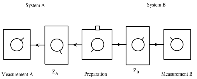
Figure 2: The preparation device here prepares a system in the form of two subsystems which go to the left and the right.

These subsystems then impinge on measurement apparatuses after passing through transformations devices which perform transformations $Z_{A}$ and $Z_{B}$. This set up can be understood to be a special case of the more generic setup shown in Fig. 1. (there is no stipulation in the case of Fig. 1. that the measurement apparatus or any of the other apparatuses be located only in one place). Assume the transformation devices are initially set to leave the subsystems unchanged. From Axiom 4 we know that there are $K_{A}K_{B}$ fiducial measurements. As discussed in Section 5, the space of positive operators for the composite system is spanned by $\hat{P}^{A}_{i}\otimes\hat{P}^{B}_{j}$ where $\hat{P}^{A}_{i}$ ($i=1$ to $K_{A}$) is a fiducial set for $A$ and $\hat{P}^{B}_{j}$ ($j=1$ to $K_{B}$) is a fiducial set for $B$. It is shown in Appendix 4 that (as we would expect) the projector $\hat{P}^{A}_{i}\otimes\hat{P}^{B}_{j}$ corresponds (i) to preparing the $i$th fiducial state at side $A$ and the $j$th fiducial state at side $B$ when the operator is regarded as representing a state, and (ii) to measuring the joint probability of obtaining a positive outcome at both ends when the $i$th fiducial measurement is performed at side $A$ and the $j$th fiducial measurement is performed at side $B$ when the operator is regarded as representing a measurement. Hence, one choice of fiducial measurements is where we simply perform the $i$th fiducial measurement on $A$ and the $j$th fiducial measurement on $B$ and measure the joint probability $p_{ij}$. The probabilities $p_{ij}$ could be put in the form of a column vector ${\bf p}_{AB}$. However, for discussing transformations, it is more convenient to put them in the form of a $K_{A}\times K_{B}$ matrix, $\tilde{p}_{AB}$, having $ij$ entry $p_{ij}$. It is easy to convert between these two ways of describing the state. We could regard both the preparation apparatus and measurement apparatus B as a preparation apparatus preparing states of subsystem $A$. If we perform the $j$th fiducial measurement on system $B$ and take only those cases where we obtain a positive result for this measurement preparing the null state otherwise then the resulting state of system $A$ will be given by a vector equal to the $j$th column of $\tilde{p}_{AB}$ (since these probabilities are equal to the probabilities that would be obtained for the fiducial measurements on $A$ with this preparation). Hence, the columns of $\tilde{p}_{AB}$ must transform under $Z_{A}$. Similarly, the rows of $\tilde{p}_{AB}$ must transform under $Z_{B}$. Hence, when the transformation devices in Fig. 2. are active, we have

$$\tilde{p}_{AB}\rightarrow Z_{A}\tilde{p}_{AB}Z_{B}^{T}$$ (97)

If the state is represented by $\tilde{r}_{AB}$ where

$$\tilde{p}_{AB}=D_{A}\tilde{r}_{AB}D_{B}^{T}$$ (98)

then this equation becomes

$$\tilde{r}_{AB}\rightarrow X_{A}\tilde{r}_{AB}X_{B}^{T}$$ (99)

where

$$X_{A}=D^{-1}_{A}Z_{A}D_{A}$$ (100)

and similarly for $B$. It is easy to see that this is the correct transformation equation in quantum theory (we have dropped the $A$ and $B$ superscripts).

$$\begin{array}[]{rcl}p^{ij}_{AB}&\!\!\!\rightarrow&{\rm tr}[\hat{P}_{i}\otimes\hat{P}_{j}\$_{A}\otimes\$_{B}(\hat{\rho})]\\ {}\hfil&=&{\rm tr}[\hat{P}_{i}\otimes\hat{P}_{j}\$_{A}\otimes\$_{B}(\sum_{kl}\hat{P}_{k}\otimes\hat{P}_{l}r^{kl})]\\ {}\hfil&=&\sum_{kl}{\rm tr}[\hat{P}_{i}\otimes\hat{P}_{j}\$_{A}(\hat{P}_{k})\otimes\$_{B}(\hat{P}_{l})]r^{kl}\\ {}\hfil&=&\sum_{kl}{\rm tr}[\hat{P}_{i}\$_{A}(\hat{P}_{k})]r_{AB}^{kl}{\rm tr}[\hat{P}_{i}\$_{B}(\hat{P}_{l})]\end{array}$$ (101)

which, using (96), gives (97) and (99). The steps in (101) can be read backwards. Hence, from (97), we obtain the tensor product structure for describing composite systems.

We will say that $Z_{A}$ is completely positive iff

$$\tilde{p}_{AB}\rightarrow Z_{A}\tilde{p}_{AB}$$ (102)

maps all allowed states of the composite system $AB$ to states which are also allowed states for any dimension $N_{B}$. The only constraint on transformation matrices $Z$ is that they transform states in $S$ to states in $S$. This means that probabilities must remain bounded by 0 and 1. Hence,

1. $Z$ must not increase the normalization coefficient of states.

2. $Z$ must be completely positive.

Condition 2 is necessary since any system could always be a subsystem of some larger system. The transformations deduced from the axioms are subject to the equivalent constraints for $\$$ listed in Section 5. They preserve Hermitivity since the transformation matrix $Z$ is real (and hence ${\bf p}$ remains real). They do not increase the trace (point 1. above). They are linear and they must be completely positive (point 2. above). Hence, the most general type of transformation consistent with the axioms is the most general transformation of quantum theory. As noted in section 5, this gives us unitary evolution and von Neumann projection as special cases.

8.9 The state after a measurement

It is possible that, after a measurement, a quantum system emerges from the measurement apparatus. In such cases the measurement apparatus is also behaving as a transformation apparatus. We can think of the state as emerging into a different channel for each measurement outcome. Associated with each outcome, $l$, of the measurement will be a certain transformation, $Z_{l}\in\Gamma$, on the state. The probability of any given outcome will not, in general, be equal to 1. Hence, the transformation must reduce the normalization coefficient associated with the state to a value consistent with the probability of obtaining that outcome. This condition is

$${\bf r}^{I}\cdot Z_{l}{\bf p}={\bf r}_{l}\cdot{\bf p}~{}~{}~{}~{}{\rm for~{}all~{}}{\bf p}\in S$$ (103)

Furthermore, we can consider all these channels taken together. In this case the effective transformation is given by $\sum_{l}Z_{l}$. It is necessary that this also belongs to the allowed set of transformations, $\Gamma$, and that it does not change the normalization coefficient associated with the state. This second condition can be written

$$\bigg{(}\sum_{l}Z_{l}\bigg{)}^{T}{\bf r}^{I}={\bf r}^{I}$$ (104)

This is equivalent to constraint

$${\rm tr}\sum_{l}\$(\hat{\rho})={\rm tr}(\hat{\rho})~{}~{}~{}{\rm for~{}all}~{}~{}~{}\hat{\rho}$$ (105)

Since completely positive operators can be written as $\$(\hat{\rho})=\sum_{l}\hat{M}_{l}\hat{\rho}\hat{M}_{l}^{\dagger}$ this equation can be shown to be equivalent to

$$\sum_{l}\hat{M}_{l}^{\dagger}\hat{M}_{l}=\hat{I}$$ (106)

which is the usual quantum constraint on superoperators associated with measurements [14, 15].

The two equations (103,104) which constrain the possible transformations of the state after measurement apply equally well to classical probability theory. This may suggest a new approach to the measurement problem in quantum theory.

9 Infinite dimensional spaces

There are two types of infinite dimensional space - countable and continuous dimensional. The countable infinite dimensional spaces are accounted for by these axioms since such systems are characterized by the property that any finite subspace obeys quantum theory. It is not so clear what the status of continuous dimensional spaces is. Such spaces can always be modeled arbitrarily well by a countable infinite dimensional Hilbert space. However, there are certain mathematical subtleties associated with the continuous case which we have not considered here. Nevertheless, it is clear that the classical continuous case violates the axioms even though there are continuous paths between states since the continuity axiom (Axiom 5) must also apply to finite subspaces (by Axiom 3) and for these there are no continuous transformations.

While continuous dimensional spaces play a role in some applications of quantum theory it is worth asking whether we expect continuous dimensional spaces to appear in a truly fundamental physical theory of nature. Considerations from quantum gravity suggest that space is not continuous at the planck scale and that the amount of information inside any finite volume is finite implying that the number of distinguishable states is countable. Given the mathematical difficulties that appear with continuous dimensional Hilbert spaces it is also natural to ask what our motivation for considering such spaces was in the first place. Consider a classical particle which can move along a straight line. If where were not a continuous infinity of distinguishable positions for the particle then the only way the particle could move would be to jump from one position to the next. It is because we do not like such discontinuities in physics that we imagine that there is a continuous infinity of distinct positions along the line. However, in quantum theory it is no longer the case that the particle would need to jump and hence the main motivation for considering the continuous dimensional case no longer pertains.

If we do, nevertheless, consider continuous dimensional spaces then there is an interesting respect in which the quantum case is superior to the classical case. Consider again a particle which can move along a straight line. Every point on the line represents a distinguishable state for the particle. Take three points $A$, $B$, and $C$ along this line where $B$ is between $A$ and $C$. In classical theory, if the particle is to move continuously through the state space from $A$ to $C$ it must pass through point $B$. However, to move continuously from $A$ to $B$ it need not pass through $C$. Hence, the pairs $AB$ and $AC$ are on an unequal footing. In quantum theory a particle can pass directly from the point $A$ to the point $C$ without going through the points in between along a continuous trajectory in the state space simply by going along the Bloch sphere corresponding to this two-dimensional subspace (such transformations do not occur in practise since Hamiltonians contain only local terms). Hence, the pairs $AB$ and $AC$ are on an equal footing. We can regard statements like “the particle is at point $B$”   as logical propositions. It is a very desirable property that pairs of propositions should be on an equal footing. Thus, in this respect, quantum theory is superior.

On the other hand, even in the quantum case, continuous dimensional spaces appear to have a topological relationship between infinitesimally displaced distinguishable states which is different to the topological relationship between finitely displaced distinguishable states. This is hard to reconcile with the notion that any pair of distinguishable states are on an equal footing and may be further support for the case against giving continuous dimensional spaces a role in any fundamental theory of nature.

10 Discussion

We have shown that quantum theory follows from five very natural axioms. If Axiom 5 (or even just the word “continuous” in Axiom 5) is dropped we obtain classical probability theory instead. It is classical probability theory that must have ‘jumps’. If a 19th century ancestor of Schroedinger had complained about “dammed classical jumps” then he might have attempted to derive a continuous theory of probability and arrived at quantum theory. Quantum theory is, in some respects, both superior to and more natural than classical probability theory (and therefore classical theories in general) since it can describe evolution for finite systems in a continuous way. Since nature is quantum, not classical, it is to be expected that quantum theory is ultimately the more reasonable theory.

There are many reasons to look for better axiomatic formulations of quantum theory.

• Aesthetics. A theory based on reasonable axioms is more appealing.

• A set of reasonable axioms provides us with a deeper conceptual understanding of a theory and is therefore more likely to suggest ways in which we could extend the domain of the theory or modify the axioms in the hope of going beyond quantum theory (for example, to develop quantum gravity).

• This approach puts a different slant on the interpretation of quantum theory (see discussion below).

• Since the formulation of quantum theory here is closer to classical probability theory than the standard formulation, this may motivate new applications and new treatments of the theory of quantum information.

There are various ways in which this work has a bearing on interpretational matters. First, if we really believe these axioms to be reasonable then they would also apply to hidden variables and it would follow that the hidden variable substructure must look like quantum theory. We could not then use hidden variables to solve the measurement problem (since this relies on being able to give the hidden variables a classical probability interpretation). Second, we see here how successful a purely instrumentalist approach is in obtaining the structure of quantum theory. Whilst this need not contradict beliefs held by the realist since he would anyway expect quantum theory to be consistent with instrumentalist argumentation, it does require some explanation. And, third, we obtain that the most general evolution is that of a superoperator. This is capable of taking pure states to mixed states. Hence, collapse interpretations of quantum theory could be incorporated into this structure.

Acknowledgements

I am very grateful to Chris Fuchs for discussions that motivated this work and to Jeremy Butterfield, Philip Pearle, Terry Rudolph, and Jos Uffink for comments. This work is funded by a Royal Society University Research Fellowship.

Appendix 1

We will prove that the property

$$f(\lambda{\bf p}_{A}+(1-\lambda){\bf p}_{B})=\lambda f({\bf p}_{A})+(1-\lambda)f({\bf p}_{B}),$$ (107)

where $\lambda\geq 0$, implies that

$$f({\bf p})=\sum_{\alpha}a_{\alpha}f({\bf p}_{\alpha})$$ (108)

where

$${\bf p}=\sum_{\alpha}a_{\alpha}{\bf p}_{\alpha}$$ (109)

if

$${\bf p}_{\alpha},{\bf p}\in S~{}~{}~{}{\rm for~{}all}~{}~{}~{}\alpha$$

for all $a_{\alpha}$ where $S$ is the set of allowed ${\bf p}$. First note that putting ${\bf p}_{A}={\bf 0}$ gives

$$f(\lambda{\bf p})=\lambda f({\bf p})$$ (110)

for $0\leq\lambda\leq 1$. We can write $\gamma=1/\lambda$ and ${\bf p}^{\prime\prime}={\bf p}/\lambda$. Then we obtain

$$f(\gamma{\bf p}^{\prime\prime})=\gamma f({\bf p}^{\prime\prime})$$ (111)

where $1\leq\gamma$. Hence,

$$f(\nu{\bf p})=\nu f({\bf p})$$ (112)

if $\nu\geq 0$. This only follows from (107) if ${\bf p},\nu{\bf p}\in S$. However, if this is not the case, then the equation does not correspond to any physical situation. Hence, we are free to impose that (112) is true for all ${\bf p}$. In those cases where ${\bf p},\nu{\bf p}\in S$ is not satisfied the equation has no physical significance anyway.

Let $f_{I}$ pertain to that measurement that simply checks to see that a non-null result has been recorded (we call this the identity measurement). We will write $f_{I}({\bf p})=\mu$. We define the normalized state $\tilde{\bf p}$ by $\mu\tilde{\bf p}={\bf p}$ such that $f_{I}(\tilde{\bf p})=1$ (using (112)).

We can normalize each of the states in (109) such that

$$\mu\tilde{\bf p}=\sum_{\alpha}a_{\alpha}\mu_{\alpha}\tilde{\bf p}_{\alpha}$$ (113)

We are free to choose the fiducial measurement corresponding to the first component of the state vector ${\bf p}$ to be the identity measurement. Hence, reading off the first component from (113) we obtain

$$\mu=\sum_{\alpha}a_{\alpha}\mu_{\alpha}$$ (114)

Let $\alpha\in A_{\pm}$ if $a_{\alpha}$ is $\pm$ve and define

$$\nu=\mu+\sum_{\alpha\in A_{-}}|a_{\alpha}|\mu_{\alpha}=\sum_{\alpha\in A_{+}}a_{\alpha}\mu_{\alpha}$$ (115)

We can rearrange (113)

$${\mu\over\nu}\tilde{\bf p}+\sum_{\alpha\in A_{-}}{|a_{\alpha}|\mu_{\alpha}\over\nu}\tilde{\bf p}_{\alpha}=\sum_{\alpha\in A_{+}}{a_{\alpha}\mu_{\alpha}\over\nu}\tilde{\bf p}_{\alpha}$$ (116)

Each coefficient is positive and the coefficients on each side add to 1. Hence we can apply (107)

$${\mu\over\nu}f(\tilde{\bf p})+\sum_{\alpha\in A_{-}}{|a_{\alpha}|\mu_{\alpha}\over\nu}f(\tilde{\bf p}_{\alpha})=\sum_{\alpha\in A_{+}}{a_{\alpha}\mu_{\alpha}\over\nu}f(\tilde{\bf p}_{\alpha})$$ (117)

Rearranging this using (112) gives (108) as required.

We see that (108) holds whenever the arguments of $f$ in each term correspond to physical states. If these arguments do not all correspond to physical states then the equation does not correspond to any physical situation. For mathematical simplicity we will impose that (108) still holds in such cases.

Appendix 2

In this appendix we show that any strictly increasing function having the completely multiplicative property

$$K(mn)=K(m)K(n),$$ (118)

where $n$ takes only positive integer values, is of the form $K(n)=n^{\alpha}$. First put $m=n=1$ into (118). We obtain that $K(1)=0,1$. Put $m=1$ into (118). If $K(1)=0$ then $K(n)=0$ for all $n$. But this is not strictly increasing. Hence we must have $K(1)=1$. The argument $n$ can be factorized into primes: $n=p_{1}^{k_{1}}p_{2}^{k_{2}}\dots$ where $p_{i}$ is the $i$th prime and the $k_{i}$’s are integers. It follows from the completely multiplicative property that

$$K(n)=\prod_{i}K^{k_{i}}(p_{i})$$ (119)

Hence, the function $K(n)$ is completely determined by its values at the primes. Now consider two primes $p$ and $q$. Define $\alpha$ by

$$K(p)=p^{\alpha}$$ (120)

Note that $K(p)>1$ since $K(n)$ is a strictly increasing function and hence $\alpha>0$. Define $a$ by

$$K(q)=aq^{\alpha}$$ (121)

Introduce the integer $t$ which we will allow to take any positive value. Then define $s$ by

$$p^{s}>q^{t}>p^{s-1}$$ (122)

From the fact that $K(n)$ is strictly increasing we have

$$K(p^{s})>K(q^{t})>K(p^{s-1})$$ (123)

Hence,

$$p^{\alpha s}>a^{t}q^{\alpha t}>p^{\alpha(s-1)}$$ (124)

Define $\widetilde{s}$ by

$$p^{\widetilde{s}}=q^{t}$$ (125)

Comparing with (122) we have

$$\widetilde{s}+1>s>\widetilde{s}>s-1>\widetilde{s}-1$$ (126)

Hence, (124) gives

$$p^{\alpha(\widetilde{s}+1)}>a^{t}q^{\alpha t}>p^{\alpha(\widetilde{s}-1)}$$ (127)

(we have used the fact that $\alpha>0$). Using (125) we obtain

$$p^{\alpha}>a^{t}>p^{-\alpha}$$ (128)

This must be true for all $t$. However, $a^{t}$ can only be bounded from above and below if $a=1$. Hence, $K(q)=q^{\alpha}$. This applies to any pair of primes, $p$ and $q$, and hence $K(n)=n^{\alpha}$.

Appendix 3

In this appendix we will prove a number of related important results some of which are used in the main part of the paper.

The set of reversible transformations is represented by the set, $\Gamma^{\rm reversible}$, of invertible matrices $Z$ in $\Gamma$ whose inverses are also in $\Gamma$. These clearly form a representation of a group. In fact, since, by Axiom 5, this group is continuous and the vectors ${\bf p}$ generated by the action of the group remain bounded, $\Gamma^{\rm reversible}$ is a representation of a compact Lie group. It can be sown that all real representations of a compact Lie group are equivalent (under a basis change) to a real orthogonal representation [21]. Let us perform such a basis change. Under this basis change assume that $Z\in\Gamma$ is transformed to $Y\in\Omega$ and ${\bf p}_{S}\in S$ is transformed to ${\bf q}\in Q$. The formula $p_{\rm meas}={\bf r}\cdot{\bf p}$ becomes

$$p_{\rm meas}={\bf s}\cdot{\bf q}$$ (129)

where ${\bf s}$ now represents the measurement (and is obtainable from ${\bf r}$ by a basis change). If a transformation device is present then we have

$$p_{\rm meas}={\bf s}^{T}Y{\bf q}$$ (130)

We can regard $Y$ as transforming the state or, alternatively, we can regard it as part of the measurement apparatus. In this case we have ${\bf s}\rightarrow Y^{T}{\bf s}$. If we now restrict our attention to reversible transformations then $Y\in\Omega^{\rm reversible}$. But this is an orthogonal representation and hence $Y^{T}\in\Omega^{\rm reversible}$. Therefore, with this representation, both states ${\bf q}$ and measurements ${\bf s}$ are acted on by elements of $\Omega^{\rm reversible}$.

A3.1

In this Appendix section we will prove that

$$Z_{W}^{T}{\bf r}^{I_{W}}={\bf r}^{I_{W}}~{}~{}~{}{\rm for~{}all}~{}~{}~{}Z_{W}\in\Gamma_{W}^{\rm reversible}$$ (131)

where ${\bf r}^{I_{W}}$ is the identity measurement for the subspace $W$ and $\Gamma_{W}^{\rm reversible}$ is the set of reversible transformations which map states in the subspace $W$ to states in $W$ – such transformations must exist by Axiom 3. We can work in the basis for which the transformations are orthogonal introduced above. Then we wish to prove

$$Y^{T}_{W}{\bf s}^{I_{W}}={\bf s}^{I_{W}}~{}~{}~{}{\rm for~{}all}~{}~{}~{}Y_{W}\in\Omega_{W}^{\rm reversible}$$ (132)

Working in this basis we can write any state in the subspace $W$ as

$${\bf q}=a{\bf s}^{I_{W}}+{\bf x}$$ (133)

where ${\bf x}$ is orthogonal to ${\bf s}^{I}$. The normalization of this state is fixed by $a$. Let $K_{W}$ be the number of degrees of freedom associated with the subspace $W$. Once the normalization coefficient has been fixed there are $K_{W}-1$ degrees of freedom left corresponding to the $K_{W}-1$ dimensions of the vector space orthogonal to ${\bf s}^{I_{W}}$ for states in $W$ which is spanned by possible ${\bf x}$. There must be at least one direction in this vector space for which both ${\bf x}$ and $\gamma{\bf x}$, where $\gamma\not=1$, are permissible vectors (corresponding to allowed states). To see this assume the contrary. Thus assume that for each direction ${\bf x}/|{\bf x}|$ there is only one allowed length of vector. Such a constraint would remove one degree of freedom leaving $K_{W}-2$ degrees of freedom which contradicts our starting point that there are $K_{W}-1$ degrees of freedom associated with states with a particular normalization coefficient. Consider such an ${\bf x}$ for which $\gamma{\bf x}$ is also permissible. Now

$${\bf s}^{I_{W}}\cdot Y_{W}{\bf q}={\bf s}^{I_{W}}\cdot{\bf q}$$ (134)

since the reversible transformation $Y_{W}$ does not change the normalization coefficient of the state and ${\bf q}$ is in $W$ both before and after the transformation. Using (133) this becomes

$$a{\bf s}^{I_{W}}\cdot Y_{W}{\bf s}^{I_{W}}+{\bf s}^{I_{W}}\cdot Y_{W}{\bf x}=a{\bf s}^{I_{W}}\cdot{\bf s}^{I_{W}}$$ (135)

This equation must also apply when ${\bf x}$ is replaced by $\gamma{\bf x}$.

$$a{\bf s}^{I_{W}}\cdot Y_{W}{\bf s}^{I_{W}}+\gamma{\bf s}^{I_{W}}\cdot Y_{W}{\bf x}=a{\bf s}^{I_{W}}\cdot{\bf s}^{I_{W}}$$ (136)

Subtracting these two equations tells us that the second term on the LHS vanishes. Hence

$${\bf s}^{I_{W}}\cdot Y_{W}{\bf s}^{I_{W}}={\bf s}^{I_{W}}\cdot{\bf s}^{I_{W}}$$ (137)

Now, the transformation $Y_{W}$ is orthogonal and hence length preserving and thus (132) follows.

It follows that

$$Y^{T}{\bf s}^{I}={\bf s}^{I}~{}~{}~{}{\rm for~{}all}~{}~{}~{}Y\in\Omega^{reversible}$$ (138)

where ${\bf s}^{I}$ is the identity measurement in this new basis (written as ${\bf r}^{I}$ in the usual basis). This property is to be expected since reversible transformations leave the normalization coefficient of a state unchanged.

A3.2

It is clearly the case that

$$Z_{W}{\bf p}\in W~{}~{}~{}{\rm if}~{}~{}~{}{\bf p}\in W~{}~{}~{}{\rm and}~{}~{}~{}Z_{W}\in\Gamma_{W}^{\rm reversible}$$ (139)

It is also the case that

$$Z_{W}{\bf p}\in\overline{W}~{}~{}~{}{\rm if}~{}~{}~{}{\bf p}\in\overline{W}~{}~{}~{}{\rm and}~{}~{}~{}Z_{W}\in\Gamma_{W}^{\rm reversible}$$ (140)

where $\overline{W}$ is the complement subspace of $W$. This follows immediately since ${\bf p}\in\overline{W}$ iff ${\bf r}^{I_{W}}\cdot{\bf p}=0$. But if this is true then, since $Z_{W}^{T}{\bf r}^{I_{W}}={\bf r}^{I_{W}}$, it is also true that ${\bf r}^{I_{W}}\cdot Z_{W}{\bf p}=0$. Hence, $Z_{W}{\bf p}\in\overline{W}$.

A3.3

We will now prove that we can choose $Z_{W}$ such that $Z_{W}{\bf p}_{n}={\bf p}_{n}$ for $n\in\overline{W}$. Define $W^{\prime}(m)$ to be the set containing all the elements of $W$ plus the first $m$ elements of $\overline{W}$. Consider only states constrained to the subspace $W^{\prime}(1)$ and consider the set $\Gamma^{\rm reversible}_{W^{\prime}(1)}$ of reversible transformations which map states in $W^{\prime}(1)$ back into $W^{\prime}(1)$. The subspace $W$ is a subspace of $W^{\prime}(1)$. Hence, by Axiom 3, there must exist a subset of $\Gamma^{\rm reversible}_{W^{\prime}(1)}$ which map states in $W$ back into $W$. By the result in A3.2 these transformations must leave the basis state ${\bf p}_{m_{1}}$ unchanged (where $m_{1}$ is the first entry of $\overline{W}$) since this is the only normalized state in $W^{\prime}(1)$ and the complement of $W$. We can now run the same argument taking $W^{\prime}(2)$ to be our system and so on. In this way we establish that we can find a transformations $Z_{W}$ which have the desired property.

A3.4

In this appendix subsection we show that one possible choice of fiducial measurements are those identified in Section 8.2. Consider the set $\Gamma_{mn}^{\rm reversible}$ of reversible transformations that transform states in the subspace $W_{mn}$ to states in the same subspace (where $W_{mn}$ is the subspace associated with the $m$th and the $n$th basis vectors). It follows from the property established in A3.2 that

$${\bf r}^{T}_{n}Z_{mn}{\bf p}=0~{}~{}~{}~{}{\rm if}~{}~{}~{}~{}{\bf p}\in\overline{W}_{mn}$$ (141)

We can regard the transformation device as part of the measurement apparatus (rather than regarding it as acting on the state). In this case we have

$${\bf r}_{n}\rightarrow Z^{T}_{mn}{\bf r}_{n}$$ (142)

We can choose two particular transformations $Z_{mnx}$ and $Z_{mny}$ to provide us with the two extra needed fiducial measurements, ${\bf r}_{mnx}$ and ${\bf r}_{mny}$ respectively, for each two-dimensional subspace. The vectors ${\bf r}_{m}$, ${\bf r}_{n}$, ${\bf r}_{mnx}$, and ${\bf r}_{mny}$ must be linearly independent. It follows from the fact that, for this subspace, the group of transformations is equivalent, under a basis change, to the full group of orthogonal rotations in three dimensions that we can choose $Z_{mnx}$ and $Z_{mny}$ such that this is the case. From (141) we have

$${\bf r}_{mnx}\cdot{\bf p}=0~{}~{}~{}{\rm if}~{}~{}~{}{\bf p}\in\overline{W}_{mn}$$ (143)

and similarly for ${\bf r}_{mny}$.

We will now prove that the $N^{2}$ vectors chosen in this way are linearly independent. We can do this by showing that each measurement yields information about the state that none of the others do. First, the vectors ${\bf r}_{n}$ are linearly independent of each other since there exists a vector (namely ${\bf p}_{m}$) having non-zero overlap with any given ${\bf r}_{m}$ which has zero overlap with all the other ${\bf r}_{n}$. Now we add two fiducial vectors, ${\bf r}_{mnx}$ and ${\bf r}_{mny}$, to each two-dimensional subspace $W_{mn}$ that are, by construction, linearly independent of the basis vectors already in that subspace. Since the fiducial measurements pertaining to one such two-dimensional subspace yield no information about states in any other non-overlapping two-dimensional subspace (because of (143))they must be linearly independent of the fiducial measurements in those non-overlapping subspaces. What about overlapping two-dimensional subspaces? Consider performing the measurement ${\bf r}_{mnx}$ on ${\bf p}$ in $W_{mn^{\prime}}$ where $n^{\prime}\not=n$. Since ${\bf p}$ is in $W_{mn^{\prime}}$ it follows from Axiom 3 that the measurement ${\bf r}_{mnx}$ must be equivalent to some measurement in this subspace (though only for states in this subspace). Now, if the state is actually the basis state ${\bf p}_{n^{\prime}}$ then zero probability would be recorded. This means that the measurement ${\bf r}_{mnx}$, when regarded as a measurement on $W_{mn^{\prime}}$ is actually equivalent to a measurement just on the one-dimensional subspace $W_{m}$. Hence, ${\bf r}_{mnx}$ does not yield any information about states in the subspace $W_{mn^{\prime}}$ that is not given by ${\bf r}_{m}$ and therefore the measurements ${\bf r}_{mn^{\prime}x}$ and ${\bf r}_{mn^{\prime}y}$ are linearly independent of it. Hence, the $N^{2}$ fiducial measurements are all necessary to determine the state and are therefore linearly independent.

A3.5

In this appendix subsection we show that the map between a pure state and that pure measurement identifying it is linear and invertible (recall that pure measurements are defined to be those measurements which can be obtained by acting on the basis measurement ${\bf r}_{1}$ with a reversible transformation). Using the basis for which reversible transformations are orthogonal (see introduction to this appendix) we can put

$${\bf q}=a{\bf s}^{I}+{\bf u}$$ (144)

for the state, and

$${\bf s}=b{\bf s}^{I}+{\bf v}$$ (145)

for the measurement where ${\bf u}$ and ${\bf v}$ are orthogonal to ${\bf s}^{I}$. Since $Y^{T}{\bf s}^{I}={\bf s}^{I}$ and since the group of reversible transformations, $\Omega^{\rm reversible}$, is orthogonal it follows that $Y{\bf s}^{I}={\bf s}^{I}$. Hence, transformations only effect the components of ${\bf q}$ and ${\bf s}$ orthogonal to ${\bf s}^{I}$. Using $p_{\rm meas}={\bf r}\cdot{\bf p}={\bf s}\cdot{\bf q}$ we obtain

$$p_{\rm meas}=k+{\bf v}\cdot{\bf u}$$ (146)

where $k=ab{\bf s}^{I}\cdot{\bf s}^{I}$.

Now assume that the pure measurement represented by ${\bf s}$ identifies the pure state represented by ${\bf q}$. Then $k+{\bf u}\cdot{\bf v}=1$. This probability cannot be increased by any transformation device. Hence,

$${\bf v}^{T}Y{\bf u}\leq{\bf v}^{T}{\bf u}~{}~{}~{}{\rm for~{}all}~{}~{}~{}Y\in\Omega^{\rm reversible}$$ (147)

Since the orthogonal transformation $Y$ is length preserving it would appear that the only way to satisfy this condition is if ${\bf v}$ is parallel to ${\bf u}$. This is indeed the case and is proven at the end of this appendix subsection. Hence, we can say that the state ${\bf q}=a{\bf s}^{I}+{\bf u}$ is identified by the measurement ${\bf s}=b{\bf s}^{I}+c{\bf u}$. Now apply this result to the basis state ${\bf q}_{1}$ (this corresponds to ${\bf p}_{1}$) and the basis measurement ${\bf s}_{1}$ (this corresponds to ${\bf r}_{1}$). Let $C$ be the linear map that performs scalar multiplication by a factor $\mu$ in the ${\bf s}^{I}$ direction and by a factor $\nu$ in the subspace orthogonal to ${\bf s}^{I}$. We can apply $C$ to ${\bf q}$ and $C^{-1}$ to ${\bf s}$ such that ${\bf s}_{1}={\bf q}_{1}=\alpha{\bf s}^{I}+\beta{\bf u}_{1}$ by appropriate choice of the factors $\mu$ and $\nu$. The maps $C$ and $C^{-1}$ commute with the orthogonal transformations $\Omega^{\rm reversible}$. Hence, in general, the pure state ${\bf q}=\alpha{\bf s}^{I}+Y\beta{\bf u}_{1}$ is identified by the pure measurement ${\bf s}=\alpha{\bf s}^{I}+Y\beta{\bf u}_{1}$ (i.e. represented by the same vector) as $YY^{T}=I$. Since the basis change and the maps $C$ and $C^{-1}$ are all linear and invertible it follows that the map from pure states to the pure measurements identifying them is linear and invertible.

As promised, we will now prove that ${\bf v}$ is parallel to ${\bf u}$ when a pure measurement ${\bf s}$ identifies a pure state ${\bf q}$. First consider the basis measurement ${\bf s}_{1}$ and the basis state ${\bf q}_{1}$ it identifies. Let $V_{mn}$ be the vector space spanned by the fiducial measurement vectors ${\bf s}_{m}$, ${\bf s}_{n}$, ${\bf s}_{mnx}$ and ${\bf s}_{mny}$ associated with the $mn$ subspace. It follows from $A3.4$ that these vector spaces span the full $N^{2}$ dimensional vector space. The state ${\bf q}_{1}$ can have no projection into the vector space $V_{mn}$ if $m,n\not=1$ (since ${\bf s}\cdot{\bf q}_{1}=0$ for ${\bf s}$ associated with the $mn$ subspace). Let $\widetilde{V}$ be the vector space spanned by the vector spaces $V_{1n}$ for $n=1$ to $N$. It follows from the fact that ${\bf q}_{1}$ has no projection into $V_{mn}$ for $m,n\not=1$ that ${\bf q}_{1}$ is in $\widetilde{V}$. Now the vector ${\bf s}^{I}=\sum_{n}{\bf s}_{n}$ is clearly in $\widetilde{V}$. Let $\widetilde{V}^{\prime}$ be the vector space in $\widetilde{V}$ orthogonal to ${\bf s}^{I}$. We can write ${\bf q}_{1}=a{\bf s}^{I}+{\bf u}_{1}$ where ${\bf u}_{1}$ is in the vector space $\widetilde{V}^{\prime}$. Similarly, we can write ${\bf s}_{1}=b{\bf s}^{I}+{\bf v}_{1}$. Define $V^{\prime}_{1n}$ as the vector space spanned by the fiducial measurement vectors ${\bf v}_{1}$, ${\bf v}_{n}$, ${\bf v}_{1nx}$, and ${\bf v}_{1ny}$ associated with the subspace $1n$. The vector spaces $V^{\prime}_{1n}$ for $n=1$ to $N$ span $\widetilde{V}^{\prime}$. Consider orthogonal transformations $Y_{1n}$ which leave states in the $1n$ subspace. They will also transform measurements pertaining to the $1n$ subspace to measurements still pertaining to this subspace (and thus still in $V^{\prime}_{1n}$). Since ${\bf v}_{1}$ and $Y_{1n}^{T}{\bf v}_{1}$ are both in $V^{\prime}_{1n}$ we can write (147) as

$${\bf v}_{1}^{T}Y_{1n}{\bf u}_{1}^{1n}\leq{\bf v}_{1}^{T}{\bf u}_{1}^{1n}$$ (148)

where ${\bf u}_{1}^{1n}$ is the component of ${\bf u}_{1}$ in $V^{\prime}_{1n}$. The vector space $V^{\prime}_{1n}$ is three dimensional and the action of the group of orthogonal transformations in the $1n$ subspace on ${\bf u}_{1}$ is to sweep out a sphere (since these transformations are length preserving). Hence, condition (148) can only be satisfied for all rotations $Y_{1n}$ if ${\bf u}_{1}^{1n}$ is parallel to ${\bf v}_{1}$. The vector spaces $V^{\prime}_{1n}$ span all of $\widetilde{V}^{\prime}$ and hence ${\bf u}_{1}$ has no component which is perpendicular to ${\bf v}_{1}$. This means that ${\bf v}_{1}$ is parallel to ${\bf u}_{1}$. We complete the proof by noting that a general pure measurement can be written ${\bf v}=Y{\bf v}_{1}$ and identifies the pure state ${\bf u}=Y{\bf u}_{1}$.

A3.6

It is easy to prove that $D=D^{T}$. We chose a set of pure fiducial states and we chose the fiducial measurements to be the set of pure measurements that identify these states. Hence, if we represent the fiducial states by a set of vectors ${\bf q}^{l}$ then, as proven in A3.5, we can represent the fiducial measurements by the the same vectors ${\bf s}^{k}={\bf q}^{k}$. The matrix element $D_{kl}$ is equal to the probability when the $k$th fiducial measurement is performed on the $l$th fiducial state. This is equal to ${\bf q}^{k}\cdot{\bf q}^{l}$ and hence $D=D^{T}$.

A3.7

Now we will show that the basis measurements ${\bf r}_{n}$ are all pure and, therefore, that all the fiducial measurements of $A3.4$ are pure. Consider first the case where $N=2$. Then $K=4$. The normalized states (and hence pure states) live in a three dimensional space (since we can eliminate one variable by normalization). Hence, orthogonal transformations can be regarded as rotations about an axis. We can write the basis states as

$${\bf q}_{1}=\alpha{\bf s}^{I}+\beta{\bf u}_{1}$$ (149)

$${\bf q}_{2}=\alpha{\bf s}^{I}-\beta{\bf u}_{1}$$ (150)

This follows since there exists a continuous orthogonal transformation which takes ${\bf q}_{1}$ to ${\bf q}_{2}$. This can be regarded as a rotation around a great circle. The orthogonal state ${\bf q}_{2}$ must correspond to the opposite point on this circle where ${\bf u}=-{\bf u}_{1}$ since this is the point at which ${\bf s}_{1}\cdot{\bf q}$ stops decreasing and starts increasing again. Now, we have already that

$${\bf s}_{1}=\alpha{\bf s}^{I}+\beta{\bf u}_{1}$$ (151)

We have not yet proven that ${\bf s}_{2}$ (corresponding to ${\bf r}_{2}$) is pure. However, we know that ${\bf s}_{1}+{\bf s}_{2}={\bf s}^{I}$ so we can write

$${\bf s}_{2}=\alpha^{\prime}{\bf s}^{I}-\beta{\bf u}_{1}$$ (152)

with $\alpha+\alpha^{\prime}=1$. It then follows from ${\bf s}_{1}\cdot{\bf q}_{2}={\bf s}_{2}\cdot{\bf q}_{1}=0$ that $\alpha=\alpha^{\prime}=1/2$. Hence, ${\bf s}_{2}$ is pure. This proof can be applied to the general $N$ case by considering only a two dimensional subspace. It follows from Axiom 3 that there must exist a set of invertible transformations which transform states in the $1n$ subspace to states in the same subspace. As shown in A3.1, these leave ${\bf s}^{I_{W_{1n}}}$ invariant (this is the identity measurement vector for the $1n$ subspace). Hence, we can replace ${\bf s}^{I}$ by ${\bf s}^{I_{W_{1n}}}$ throughout the above proof if we are only considering transformations in this subspace. It follows that we can transform ${\bf s}_{1}$ to ${\bf s}_{n}$ and hence the basis measurements are all pure.

Hence we can transform ${\bf s}_{1}$ to any ${\bf s}_{mnx}$ by first transforming by a reversible transformation to ${\bf s}_{n}$ and then applying the reversible transformation of A3.4 to obtain ${\bf s}_{mnx}$. Similar remarks apply to ${\bf s}_{mny}$.

Appendix 4

In this appendix we will show that the projector $\hat{P}^{A}_{i}\otimes\hat{P}^{B}_{j}$ can correspond to the measurement of the joint probability of obtaining a positive outcome for fiducial measurements $i$ at $A$ and $j$ at $B$, and to the state when the $i$th fiducial state is prepared at $A$ and the $j$th fiducial state is prepared at $B$. First, note that we can prepare $N_{A}N_{B}$ distinguishable states for the composite system by preparing basis state $m$ at $A$ and basis state $n$ at $B$. Since the composite system has $N=N_{A}N_{B}$ this represents a complete set of basis states. Further, since $K(1)=1$ all basis states must be pure (as noted at the end of Section 8.1). Hence, we can choose these basis states to correspond to the basis states of our Hilbert space $|mn\rangle$ or, equivalently, $|m\rangle\otimes|n\rangle$. As operators these basis states are $\hat{P}^{A}_{m}\otimes\hat{P}^{B}_{n}$ where $m$ ($n$) only runs over the first $N_{A}$ ($N_{B}$) values (the remaining values corresponding to the other fiducial projectors).

Now consider the $N_{B}$ dimensional subspace with basis states $|1\rangle\otimes|n\rangle$ ($n=1$ to $N_{B}$). This subspace corresponds to the case where system $A$ is prepared in basis state $1$ and system $B$ is prepared in any state. A full set of fiducial projectors can be formed for this subspace. These will take the form $\hat{P}^{A}_{1}\otimes\hat{P}^{B}_{l}$ where $l=1$ to $K_{B}$ (i.e. runs over the all values, not just the basis labels). We can do the same for the case where basis state 2 is prepared at $A$. Then we have the fiducial projectors $\hat{P}^{A}_{2}\otimes\hat{P}^{B}_{l}$ for the subspace $2n$ ($n=1$ to $N_{B}$). Indeed, we can do this for the general case in which the basis state $m$ is prepared at $A$. Now consider the pure state $\hat{P}^{A}_{1}\otimes\hat{Q}^{B}$ where $\hat{Q}^{B}$ is some arbitrary projector at $B$. This state is in the $1n$ ($n=1$ to $N_{B}$) subspace and we can perform the fiducial measurements $\hat{P}^{A}_{1}\otimes\hat{P}_{l}^{B}$ in this subspace to fully characterize this state. The probabilities obtained in making these fiducial measurements will be the same as if we prepared the state $\hat{P}^{A}_{2}\otimes\hat{Q}^{B}$ and made the fiducial measurements $\hat{P}^{A}_{2}\otimes\hat{P}_{l}^{B}$ and hence this corresponds to the same preparation at $B$. Hence, in general the projector $\hat{P}^{A}_{m}\otimes\hat{Q}^{B}$ corresponds to preparing the basis state $\hat{P}_{m}$ at $A$ and the general pure state $\hat{Q}^{B}$ at $B$. Now consider the subspace spanned by the projectors $\hat{P}^{A}_{m}\otimes\hat{Q}^{B}$ ($m=1$ to $N_{A}$) in which we prepare $\hat{Q}^{B}$ at $B$. A fiducial set for this subspace is $\hat{P}^{A}_{k}\otimes\hat{Q}^{B}$ where $k=1$ to $K_{A}$. If these fiducial measurements are made on a state $\hat{R}^{A}\otimes\hat{Q}^{B}$ where $\hat{R}^{A}$ is a projector at $A$ then we would get the same results as if the fiducial measurements $\hat{P}^{A}_{k}\otimes\hat{Q^{\prime}}^{B}$ were made on the state $\hat{R}^{A}\otimes\hat{Q^{\prime}}^{B}$. Hence, in both cases the preparation at $A$ is the same. Thus, the pure state $\hat{R}^{A}\otimes\hat{Q}^{B}$ corresponds to the case where a particular pure state $\hat{R}^{A}$ is is prepared at $A$ and the pure state $\hat{Q}^{B}$ is prepared at $B$. An analogous argument to that above can be used to show that, regarded as a measurement, the projector $\hat{R}^{A}\otimes\hat{Q}^{B}$ corresponds to measuring the joint probability with setting $\hat{R}^{A}$ at end $A$ and setting $\hat{Q}^{B}$ at end $B$. Applied to the fiducial projectors, $\hat{P}_{k}^{A}\otimes\hat{P}_{l}^{B}$, this proves our result.

References

- [1] G. Birkhoff and J. von Neumann, Ann. Math. 37, 743 (1936).
- [2] G. W. Mackey, The mathematical foundations of quantum mechanics (W. A. Benjamin Inc, New York, 1963).
- [3] J. M. Jaunch and C. Piron, Helv. Phys. Acta 36, 837 (1963); C. Piron, Helv. Phys. Acta 37, 439 (1964).
- [4] G. Ludwig, Commun. Math. Phys. 9, 1 (1968), G. Ludwig, Foundations of quantum mechanics volumes I and II (Springer-Verlag, New York, 1983 and 1985).
- [5] B. Mielnik, Commun. Math. Phys. 9, 55 (1968).
- [6] A. Lande, Am. J. Phys. 42, 459 (1974).
- [7] D. I. Fivel, Phys. Rev. A 50 2108 (1994).
- [8] L. Accardi, Il Nuovo Cimento 110B, 685 (1995).
- [9] N. P. Landsman, Int. J. of Theoretical Phys. 37, 343 (1998) and Mathematical topics between classical and quantum mechanics (Springer, New York, 1998).
- [10] B. Coecke, D. Moore, A. Wilce, Current research in operational quantum logic: algebras, categories, languages (Fundamental theories of physics series, Kluwer Academic Publishers, 2000), also available on quant-ph/0008019.
- [11] A. M. Gleason, Annals of Math 6, 885 (1957).
- [12] S. Kochen and E.P. Specher, J. Math and Mech. 17, 59 (1967).
- [13] I. Pitowsky, Lecture notes in physics 321 (Springer-Verlag, Berlin-Heildelburg 1989).
- [14] K. Kraus, States, effects, and operations: Fundamental notions of quantum theory (Springer-Verlag, Berlin, 1983); B. Schumacher, quant-ph/9604023 (appendix A); J. Preskill Lecture notes for physics 229: quantum information and computation, available at http://ww.theory.ca.tech.edu/ preskill/ph229 (see chapter 3).
- [15] M. A. Nielsen and I. L. Chuang, Quantum information and quantum information, (Cambridge University Press, 2000).
- [16] R. Schack, private communication.
- [17] D. Deutsch, private communication.
- [18] W. K. Wootters, Local accessibility of quantum states, in Complexity, entropy and the physics of information edited by W. H. Zurek (Addison-Wesley, 1990) and W. K. Wootters, Found. Phys 16, 319 (1986).
- [19] S. Weigert, Phys. Rev. Lett. 84, 802 (2000).
- [20] It has been noted by C. Caves, C. Fuchs and R. Schack in quant-ph/0104088 that difficulties in formulating a De Finetti theorem for quaternionic quantum theory stem from the fact that .
- [21] H. Boerner, Representations of groups (North-Holland publishing company, Amsterdam 1963).