[

Quantum Computing of Classical Chaos: Smile of the Arnold-Schrödinger Cat

Abstract

We show on the example of the Arnold cat map that classical chaotic systems can be simulated with exponential efficiency on a quantum computer. Although classical computer errors grow exponentially with time, the quantum algorithm with moderate imperfections is able to simulate accurately the unstable chaotic classical dynamics for long times. The algorithm can be easily implemented on systems of a few qubits.

]

A great deal of attention has been attracted recently by the possibility to perform numerical simulations on a quantum computer. The massive parallelism allowed by quantum mechanics enables to operate on an exponential number of states using a single quantum transformation, as was stressed by Feynman [1]. However, even if exponential gain may be possible in such quantum simulations, compared to the computations on classical computers, only few problems have been found where an explicit quantum algorithm displays such efficiency. The most famous of them is the factorization of large integers, for which Shor [2] constructed an explicit algorithm which is exponentially faster than any known classical algorithm. Another well-known algorithm, invented by Grover [3], also shows that quantum mechanics can enormously accelerate the search problem in an unsorted database, although the gain is not exponential. Although quantum-mechanical problems are computationally very hard for classical simulations, at present only few physical systems are known which can be simulated with exponential efficiency on a quantum computer. Such systems include certain spin lattices [4], some types of many-body systems [5], and since recently the kicked rotator model of quantum chaos [6]. The advances in the field of quantum computation [7, 8, 9] generated many proposals for the experimental realization of such a computer. This computer is viewed as a system of qubits (two-level systems) on which one-qubit rotations and two-qubit transformations allow to realize any unitary transformation in the exponentially large Hilbert space (see reviews [7, 8, 9]). At present operations with two qubits were realized with cold ions [10], and the Grover algorithm was performed on a three-qubit system built on nuclear spins in a molecule [11].

It may seem natural that quantum computers can simulate efficiently the evolution of certain quantum systems. Such systems are very hard to simulate on classical computers due to the exponentially large Hilbert space. However, there also exists a large class of classical Hamiltonian systems which are very hard to simulate accurately on a classical computer. Indeed, the systems displaying dynamical chaos are characterized by an exponential local instability of trajectories in the phase space [12, 13]. As a result, standard round-off errors of an usual computer grow exponentially with time, and give a complete change of a dynamical trajectory with given initial parameters after a few characteristic periods of the system motion. In this situation, the simulation of a full phase space density even for moderate times needs an exponential number of orbits and soon exceeds the capacity of modern classical computers. To our knowledge, the problem of performing such simulations on a quantum computer was not addressed until now. Indeed, it may look surprising that quantum mechanics may help in simulations of classical dynamics. In this paper, we show that a well-known example of classical chaotic system can be simulated on a quantum computer with exponential efficiency compared to classical algorithms. Moreover, even if due to chaos the classical errors grow exponentially with time, the quantum simulations with moderate quantum errors still enable to reproduce accurately the time evolution in the classical phase space. The resolution of this apparent paradox is rooted in the fundamental differences between classical and quantum mechanics.

One of the most famous example of classically chaotic systems is the Arnold cat map, an automorphism of the torus [12, 13]. The dynamics of the map is given by:

$$\bar{y}=y+x\;\mbox{(mod}\;\mbox{1)}\;\;,\;\;\bar{x}=y+2x\;\mbox{(mod}\;\mbox{1)}\;,$$ (1)

where bars denote the new values of the variables after one iteration. This is an area-preserving map, in which $x$ can be considered as the space variable and $y$ as the momentum. In this way, the first equation can be seen as a kick which changes the momentum $y$, while the second equation describes the free phase rotation. This map belongs to the class of Anosov systems, with homogeneous exponential divergence of trajectories and positive Kolmogorov-Sinai entropy $h=\mbox{ln}(\frac{3+\sqrt{5}}{2})\approx 0.96$. Due to this exponential instability, a typical computer round-off error of order $10^{-16}$ will change completely the position of a trajectory in the phase space torus after only 38 iterations. Although the exact dynamics of (1) is time-reversible [14], the round-off errors make it effectively irreversible after a short time.

Usually computer round-off errors are not symplectic, and destroy the area-preserving property of the map. However, it is possible to consider a discretized map which remains area-preserving after discretization. It is known that such symplectic discretization describes the continuous dynamics in the most appropriate way [15]. Such a discrete approximation remains close to the exact map dynamics up to the time scale $t_{E}\approx\ln N/h$ where $N^{2}$ is the number of points of the discretized torus, so that the discrete cells have the area $1/N^{2}$. For the cat map (1) the discretized map is especially simple, consisting of the dynamics through (1) of the $N^{2}$ points $(x_{i},y_{j})$ with $x_{i}=i/N$, $i=0,...,N-1$ and $y_{j}=j/N$, $j=0,...,N-1$. Even after discretization, the exponential instability still manifests itself through the rapid disappearance of any structure in phase space (for example the cat image) after few iterations, see Fig.1 (left). The discrete map preserves time-reversibility [14], however any small imprecision at the time of inversion destroys this reversibility as is illustrated on Fig.1 (left). Here for $N=128$, the smallest error (of one cell size) destroys reversibility already after 10 iterations. On a classical computer, one map iteration requires $O(N^{2})$ additions to simulate the evolution of a phase-space density distribution.

On the contrary, we found that on a quantum computer the discretized Arnold cat map can be simulated exponentially faster. Our quantum algorithm operates on $3n_{q}-1$ qubits. The first two quantum registers, each with $n_{q}$ qubits, describe the position $x_{i}$ and the momentum $y_{j}$ of $N^{2}$ points of the discretized classical phase space, with $N=2^{n_{q}}$. The remaining $n_{q}-1$ qubits are used as workspace. An initial classical phase space density can then be represented by a quantum state $\sum_{i,j}a_{ij}|x_{i}>|y_{j}>|0>$. The map dynamics requires additions of integers modulo (N) (modular additions). The quantum algorithm we use for this operation is similar to the one described in [16] (see also [17]). The third register holds the carries of the addition, and the result is taken modulo (N) by eliminating the last carry. One map iteration requires first adding the first register to the second, and then adding the second register to the first. After that, the coefficients $a_{ij}$ describe the classical phase space density after one map iteration. To perform these additions, $8n_{q}-12$ Toffoli gates and $8n_{q}-10$ controlled-not gates are needed per map iteration, giving a total of $16n_{q}-22$ operations for $n_{q}\geq 3$ [18]. This means that the quantum computer can iterate this classical chaotic map exponentially faster than the classical computer, which requires $O(2^{2n_{q}})$ operations per iteration. Hence, the quantum evolution obeying the Schrödinger equation describes the classical Arnold cat map, and we will call this quantum dynamics the Arnold-Schrödinger cat map.

If the quantum gates are perfect, then the quantum algorithm describes exactly the classical density evolution. But physical systems are never perfect, and to be really efficient the quantum algorithm should be stable against

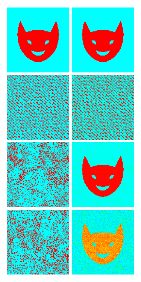
FIG. 1.: Dynamics of Arnold-Schrödinger cat simulated on a classical (left) and quantum computer (right), on a $128\times 128$ lattice. Upper row: initial distribution; second row: distributions after 10 iterations; third row: distributions at $t_{2r}=20$, with time inversion made at $t_{r}=10$; bottom row: distributions at $t_{2r}=400$, with time inversion made at $t_{r}=200$. Left: inversion is done with classical error of one cell size ($\epsilon=1/128$) at $t=t_{r}$ only; right: all quantum gates operate with quantum errors of amplitude $\epsilon=0.01$; color from blue to red gives the probability $|a_{ij}|^{2}$; $n_{q}=7$.

imperfections. In view of the exponential instability of classical computer errors in this problem, this may look rather doubtful. To study the effects of imperfections on this algorithm, we introduced some random unitary noise in the gate operations. For each gate transformation, the nondiagonal part was diagonalized, and each eigenvalue was multiplied by a random phase $\exp(i\eta)$, with $-\epsilon<\eta<\epsilon$. Here we assume that imperfections due to residual static coupling between qubits are small enough, and that the quantum computer operates below the quantum chaos border discussed in [19].

FIG. 2.: Quantum fidelity $f$ of Arnold-Schrödinger cat as a function of time $t$ for quantum errors $\epsilon=0.003,0.01,0.03$ (dashed and dotted curves from top to bottom respectively). Initial state: cat’s smile as in Fig. 1 (dashed curves) and line $x=1/2$ (dotted curves). Full curve shows the drop of fidelity when a minimal classical error is done at $t=200$ (see text).

FIG. 3.: Classical fidelity $f_{c}(2t_{e})$ vs. time $t_{e}$ when the minimal classical error ($\epsilon=1/128$) is made (full curve). Dashed curve shows the same $f_{c}$ obtained by the quantum computer with imperfections of amplitude $\epsilon=0.01$ (see text).

To investigate the stability of the algorithm with respect to quantum imperfections, we used first a time-inversion test. Namely, starting from a given classical density (representing the cat’s smile), we perform $t_{r}$ iterations forwards, then invert all momenta (time-inversion), and perform again $t_{r}$ iterations. Without imperfections, the density returns exactly to its initial distribution at $t_{2r}=2t_{r}$. On the left of Fig.1, one can see the dramatic effect of small random classical computer errors (here of size $\epsilon=1/N\approx 10^{-2}$), performed only at the moment of the time-inversion: it completely destroys reversibility after a few iterations. On the contrary, the quantum errors of similar amplitude, although present at each map iteration, practically do not affect the smile of the Arnold-Schrödinger cat after $t_{2r}=20$ iterations, and only slightly perturb it after $t_{2r}=400$. This pictorial image shows the power of quantum computation, which even in presence of relatively strong imperfections is able to simulate classical chaotic dynamics. We note that quantum systems for which the classical limit is chaotic (e.g. the kicked rotator) are also stable with respect to time inversion [20].

To be more quantitative, we computed the fidelity of the quantum state in presence of errors, namely $f(t)=|<\psi_{\epsilon}(t)|\psi_{0}(t)>|^{2}$. Here $|\psi_{0}(t)>$ is the quantum state after $t$ perfect iterations, while $|\psi_{\epsilon}(t)>$ is the quantum state after $t$ imperfect iterations. The dependence of fidelity on time is shown on Fig.2. Here we present $f(t)$ for two initial states, one representing the cat’s smile, and another a line in phase space, with $x=1/2$. The latter is especially easy to prepare, requiring only $n_{q}+1$ single-qubit rotations. The data clearly show that in both cases the fidelity drops very slowly with the number of iterations, confirming the stability of quantum dynamics. In view of the exponential growth of classical errors, this may look as a paradox. Indeed, as is illustrated in Fig.1, exponentially small classical errors of size $1/N$ destroy practically immediately any structure. The resolution of this paradox lies in the fact that a small classical error can be very large from the viewpoint of quantum mechanics. This fact is shown in Fig.2, where after a small classical error affecting only the smallest bit in the positions $x_{i},y_{j}$ the fidelity of the quantum state drops immediately to a very small value. Curiously enough, after this drop, perfect iterations of the map do not change the fidelity, although the classical error (i.e. distance between exact and perturbed orbits) starts to grow exponentially due to trajectory divergence in phase space.

In this situation, one may wonder where in the quantum dynamics is hidden the classical exponential instability. In fact, it is always present even if quantum dynamics remains stable. Indeed, the drop in the fidelity induced by classical errors depends exponentially on the moment of time $t_{e}$ when the error is made. This fact is illustrated by Fig.3, which shows the classical fidelity $f_{c}$, defined in the same way as the fidelity for quantum errors: $f_{c}(t,t_{e})=|<\psi_{e}(t,t_{e})|\psi_{0}(t)>|^{2}$ where $|\psi_{e}(t,t_{e})>$ is the quantum state after the classical error is done at time $t_{e}<t$ and $|\psi_{0}(t)>$ is the quantum state without error. This function $f_{c}(t,t_{e})$ can be also computed purely classically. As seen in Fig.2, for given $t_{e}$ and $t>t_{e}$, the fidelity $f_{c}$ remains exactly constant, since $f_{c}$ is preserved by unitary transformations. However, its value depends strongly on $t_{e}$, as is shown in Fig.3, where $f_{c}$ is computed at time $t=2t_{e}$. The data clearly show the exponential drop of classical fidelity with $t_{e}$. This reflects the existence of exponential instability in the cat map dynamics. If a time inversion with errors is done at $t_{r}=t_{e}$, as in Fig.3, then the value of $f_{c}$ gives the recovered fraction of the initial distribution (cat’s smile) at $t=2t_{r}$. This whole process can be made on the quantum computer with imperfections, and Fig.3 shows that even with imperfections the quantum computer gives practically the same classical fidelity which drops exponentially. Hence a quantum computer can simulate accurately the exponential growth of classical errors in the regime of chaos.

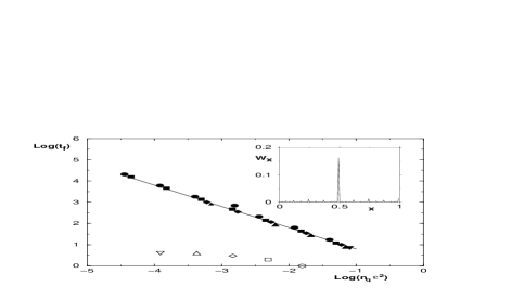
FIG. 4.: Fidelity time scale $t_{f}$ as a function of $\epsilon^{2}n_{q}$: $n_{q}=4$ (circles), $5$ (squares), $6$(diamonds), $7$ (triangles up), $8$ (triangles down)); filled symbols are for quantum errors ($0.003\leq\epsilon\leq 0.1$), open ones are for classical errors ($0.003<\epsilon<0.1$); the full line gives $t_{f}=0.63/(\epsilon^{2}n_{q})$. Inset: probability distribution $W_{x}$ in $|x>$ at the moment of return $t_{2r}=400$ for time inversion at $t_{r}=200$, and quantum imperfections $\epsilon=0.03$, for $n_{q}=7$ with $x=1/2$ at $t=0$.

To study quantitatively the dependence of the fidelity $f(t)$ on the magnitude of errors, we determine the fidelity time scale $t_{f}$ by the condition $f(t_{f})=0.5$. For quantum errors, Fig.4 shows that $t_{f}\approx 0.63/(\epsilon^{2}n_{q})$. Indeed, the probability of transition from the exact state to other states is of order $\epsilon^{2}$ for each gate operation. After $t_{f}$ map iterations, $t_{f}n_{q}$ such operations are done, so that the fidelity drops by $\epsilon^{2}n_{q}t_{f}\sim 0.5$, giving the above estimate. This estimate is rather general, and it corresponds to a general property of quantum mechanics due to which the fidelity can drop only polynomially with unitary noise and the number of imperfect gates applied. On the contrary, in the classical case $t_{f}$ extracted from the classical fidelity $f_{c}(t_{e}=t_{f})=0.5$ (see Fig.3) is of the order of $t_{f}\approx 1.4\ln(1/\epsilon)$, comparable with $t_{E}$ for $\epsilon\sim 1/N$.

We stress that the Arnold-Schrödinger cat is very simple to implement. For example, one map iteration with $n_{q}=4$ requires only $11$ qubits and $42$ gates, and can be experimentally realized in the near future. The time inversion test explained above can be performed experimentally and be used to test the actual accuracy of the quantum computer. Indeed, an initial distribution in the form of the line $x=1/2$ can be easily prepared, and from a few measurements of the $|x>$ register at the return moment $t=t_{2r}$ one can estimate the probability of non-return which allows to determine the amplitude of quantum errors. The inset in Fig.4 shows an example of such final state. It is interesting to note that $n_{q}=20$ needs only $59$ qubits and will permit to make computations unaccessible to nowadays supercomputers, with memory size $\approx 200$ Go. In this regime global quantities inaccessible by classical computation can be obtained. For example, the main harmonics of the density distribution can be obtained with the help of the quantum Fourier transform followed by a few measurements.

In conclusion, our study of the Arnold-Schrödinger cat dynamics shows that classical unstable motion, for which classical computers demonstrate exponential sensibility to errors, can be simulated accurately with exponential efficiency by a realistic quantum computer.

We thank the IDRIS in Orsay and the CalMiP in Toulouse for access to their supercomputers.

REFERENCES

- [1] R. P. Feynman, Found. Phys. 16, 507 (1986).
- [2] P. W. Shor, in Proc. 35th Annu. Symp. Foundations of Computer Science (ed. Goldwasser, S. ), 124 (IEEE Computer Society, Los Alamitos, CA, 1994).
- [3] Lev K. Grover, Phys. Rev. Lett. 79, 325 (1997).
- [4] A. Sørensen and K. Mølmer, Phys. Rev. Lett. 83, 2274 (1999).
- [5] S. Lloyd, Science 273, 1073 (1996).
- [6] B. Georgeot and D. L. Shepelyansky, quant-ph/0010005.
- [7] D. P. Di Vincenzo, Science 270, 255 (1995).
- [8] A. Ekert and R. Josza, Rev. Mod. Phys. 68, 733 (1996).
- [9] A. Steane, Rep. Progr. Phys. 61, 117 (1998).
- [10] C. Monroe, D. M. Meekhof, B. E. King, W. M. Itano and D. J. Wineland, Phys. Rev. Lett. 75, 4714 (1995).
- [11] L. M. Vandersypen, M. Steffen, M. H. Sherwood, C. S. Yannoni, G. Breyta and I. L. Chuang, Appl. Phys. Lett. 76, 646 (2000).
- [12] V. I. Arnold and A. Avez, Ergodic Problems of Classical Mechanics, Benjamin, N. Y. (1968).
- [13] A. Lichtenberg and M. Lieberman, Regular and Chaotic Dynamics, Springer, N.Y. (1992).
- [14] The time-inversion physically can be viewed as inversion of all momenta half-way between the kicks. The iteration with time-inversion gives , . After that, iterations of (1) give the evolution backwards.
- [15] F. Rannou, Astron. Astrophys. 31, 289 (1974); D. J. D. Earn and S. Tremaine, Physica D 56, 1 (1992).
- [16] V. Vedral, A. Barrenco and A. Ekert, Phys. rev. A 54, 147 (1996).
- [17] D. Beckman, A. N. Chari, S. Devabhaktuni and J. Preskill, Phys. Rev. A 54, 1034 (1996); C. Miquel, J. P. Paz and R. Perazzo, Phys. Rev. A 54, 2605 (1996).
- [18] The time-inversion in the quantum algorithm requires one-qubit rotation (, ), plus Toffoli and controlled-not gates, and hence is also exponentially fast.
- [19] B. Georgeot and D. L. Shepelyansky, Phys. Rev. E 62, 3504 (2000); ibid. 62, 6366 (2000).
- [20] D. L. Shepelyansky, Physica D 8, 208 (1983).