An Analysis of Completely-Positive Trace-Preserving Maps on $\mathcal{M}_{2}$

Abstract

We give a useful new characterization of the set of all completely positive, trace-preserving maps $\Phi:\mathcal{M}_{2}\rightarrow\mathcal{M}_{2}$ from which one can easily check any trace-preserving map for complete positivity. We also determine explicitly all extreme points of this set, and give a useful parameterization after reduction to a certain canonical form. This allows a detailed examination of an important class of non-unital extreme points that can be characterized as having exactly two images on the Bloch sphere.

We also discuss a number of related issues about the images and the geometry of the set of stochastic maps, and show that any stochastic map on ${\mathcal{M}}_{2}$ can be written as a convex combination of two “generalized” extreme points.

Key Words: Completely positive maps, stochastic maps, quantum communication, noisy channels, Bloch sphere, states, .

MR Classification. 47L07, 81P68, 15A99, 46L30, 46L60, 94A40

1 Introduction

1.1 Background

Completely positive, trace-preserving maps arise naturally in quantum information theory and other situations in which one wishes to restrict attention to a quantum system that should properly be considered a subsystem of a larger system with which it interacts. In such situations, the system of interest is described by a Hilbert space ${\cal H}_{1}$ and the larger system by a tensor product ${\cal H}={\cal H}_{1}\otimes{\cal H}_{2}$. States correspond to density matrices, where a density matrix $\rho$ is a positive semi-definite operator on ${\cal H}_{1}$ with $\hbox{Tr}\rho=1$. The result of the “noisy” interaction with the larger system is described by a stochastic map $\Phi:{\cal B}({\cal H}_{1})\rightarrow{\cal B}({\cal H}_{1})$ that takes $\rho$ to another density matrix $\Phi(\rho)$. Since $\Phi(\rho)$ should also be a density matrix, $\Phi$ must be both trace-preserving and positivity preserving. However, the latter is not enough, since $\Phi(\rho)$ is the result of a positivity-preserving process on the larger space of operators in ${\cal B}({\cal H}_{1}\otimes{\cal H}_{2})={\cal B}({\cal H}_{1})\otimes{\cal B}({\cal H}_{2})$. This is precisely the condition that $\Phi$ be completely positive.

The notion of complete positivity was introduced in the more general context of linear maps $\Phi:{\cal A}_{1}\rightarrow{\cal A}_{2}$ on $C^{*}$-algebras where the condition can be stated as the requirement that $\Phi\otimes I_{\mathcal{M}_{n}}:{\cal A}_{1}\otimes\mathcal{M}_{n}\rightarrow{\cal A}_{2}\otimes\mathcal{M}_{n}$ is positivity preserving for all $n$, where $\mathcal{M}_{n}$ denotes the algebra of complex $n\times n$ matrices. Stinespring showed that a completely positive map always has a representation of the form $\pi_{2}[\Phi(A)]=V^{*}\pi_{1}(A)V$ where $\pi_{1}$ and $\pi_{2}$ are representations of the algebras ${\cal A}_{1},{\cal A}_{2}$ respectively. Kraus [15, 16] and Choi [4] showed that this leads to the more tangible condition that there exists a set of operators $A_{k}$ such that

$$\Phi(\rho)=\sum_{k}A_{k}^{\dagger}\rho A_{k}.$$ (1)

(where we henceforth follow the physics convention of using $\dagger$ to denote the adjoint of an operator.) The condition that $\Phi$ is trace-preserving can then be written as $\sum_{k}A_{k}A_{k}^{\dagger}=I$. When this condition is also satisfied, (1) can also be used [16, 19] to find a representation of $\Phi$ in terms of a partial trace on a larger space.

The operators in (1) are often referred to as “Kraus operators” because of his influential work [15, 16] on quantum measurement in which he emphasized the role of completely positive maps. Recognition that such maps play a natural role in the description of quantum systems goes back at least to Haag and Kastler [7]. It is worth noting that this representation is highly non-unique, and that this non-uniqueness can not be eliminated by simple constraints. In particular, one can find extreme maps with at least two two different Kraus representations each of which uses only the minimal number of Kraus operators. An example is given in Section 3.4. The representation (1) was obtained independently by Choi [4] in connection with important tests, upon which this paper is based, for complete-positivity and extremality in the case of maps on $\mathcal{M}_{n}$.

However, Choi’s condition and all of the representations discussed above require, at least implicitly, consideration of the map $\Phi\otimes I_{\mathcal{M}_{n}}$ on a larger space. (In quantum information theory this problem is sometimes avoided by defining a stochastic map, or channel, in terms of its Kraus operators as in (1); however, this approach has thus tended to focus attention on a rather limited set of channels.) One would like to find a simple way to characterize completely positive maps in terms of their action on the algebra ${\cal B}({\cal H}_{1})$ of the subsystem. The purpose of this paper is to obtain such a characterization in the special case of trace-preserving maps on ${\cal B}({\cal H}_{1})=\mathcal{M}_{2}$. This leads to a complete description of their extreme points, and a useful parameterization of the stochastic maps and their extreme points. Although the two-dimensional case ${\cal H}_{1}={\bf C}^{2}$ may seem rather special, it is of considerable importance because of its role in quantum computation and quantum communication.

If, in addition to being trace-preserving, a completely positive map $\Phi$ is unital, i.e., $\Phi(I)=I$, we call $\Phi$ bistochastic. This terminology for maps that are both unital and stochastic was introduced in [2].

1.2 Notation

First, we note that for a linear map $\Phi$, its adjoint, which we denote $\widehat{\Phi}$ (to avoid confusion with the operator adjoint of a specific image) can be defined with respect to the Hilbert-Schmidt inner product $\langle A,B\rangle=\hbox{Tr}A^{\dagger}B$ so that $\hbox{Tr}\,[\Phi(A)]^{\dagger}B=\hbox{Tr}\,A^{\dagger}\widehat{\Phi}(B)$. It is easy to verify that the Kraus operators for $\widehat{\Phi}$ are the adjoints of those for $\Phi$ so that (1) implies $\widehat{\Phi}(\rho)=\sum_{k}A_{k}\rho A_{k}^{\dagger}$, and that $\Phi$ is trace-preserving if and only if $\widehat{\Phi}(I)=I$, i.e., if $\widehat{\Phi}$ is unital.

In order to state our results in a useful form, we recall that the identity and Pauli matrices $\{I,\sigma_{x},\sigma_{y},\sigma_{z}\}$ form a basis for $\mathcal{M}_{2}$ where

$$\sigma_{x}=\left(\begin{array}[]{cc}0&1\\ 1&0\end{array}\right)~{}~{}\sigma_{y}=\left(\begin{array}[]{cc}0&-i\\ i&0\end{array}\right)~{}~{}\sigma_{z}=\left(\begin{array}[]{cc}1&0\\ 0&-1\end{array}\right).$$

Every density matrix can be written in this basis as $\rho={{\textstyle\frac{1}{2}}}[I+{\bf w}\cdot{\bf\sigma}]$ with ${\bf w}\in{\bf R}^{3}$ and $|{\bf w}|\leq 1$. Thus, the set of density matrices, which we shall denote by ${\mathcal{D}}$, can be identified with the unit ball in ${\bf R}^{3}$ and the pure states (rank one projections) lie on the surface known as the “Bloch sphere.” Since $\Phi$ is a linear map on $\mathcal{M}_{2}$, it can also be represented in this basis by a unique $4\times 4$ matrix ${\bf T}$, and $\Phi$ is trace-preserving if and only if the first row satisfies $t_{1k}=\delta_{1k}$, i.e., ${\bf T}=\left(\begin{array}[]{cc}1&{\bf 0}\\ {\bf t}&{{\rm T}}\end{array}\right)$ where ${\rm T}$ is a $3\times 3$ matrix (and ${\bf 0}$ and ${\bf t}$ are row and column vectors respectively) so that

$$\Phi(w_{0}I+{\bf w}\cdot\sigma)=w_{0}I+({\bf t}+{\rm T}{\bf w})\cdot\sigma.$$ (3)

The ${\bf T}$-matrix corresponding to $\widehat{\Phi}$ is ${\bf T}^{\dagger}$.

When $\Phi$ is also positivity-preserving, it maps the subspace of self-adjoint matrices in $\mathcal{M}_{2}$ into itself, which implies that $\bf T$ is real. King and Ruskai [13] showed that any such map can be reduced, via changes of basis in ${\bf C^{2}}$, to the form

$${\bf T}=\pmatrix{1&0&0&0\cr t_{1}&\lambda_{1}&0&0\cr t_{2}&0&\lambda_{2}&0\cr t_{3}&0&0&\lambda_{3}}.$$ (4)

Because a unitary change of basis $\rho\rightarrow V\rho V^{\dagger}$ on ${\bf C^{2}}$ is equivalent to a 3-dimensional rotation ${\bf w}\rightarrow R{\bf w}$ acting on the Pauli matrices, this is equivalent to

$$\Phi(\rho)=U\Big{[}{\Phi}_{{\bf t},{\bf\Lambda}}\big{(}V\rho V^{\dagger}\big{)}\Big{]}U^{\dagger},$$ (5)

where $U,V\in U(2)$ and $\Phi_{{\bf t},{\bf\Lambda}}$ denotes the map corresponding to (4). The reduction to (4) is obtained by applying a modification of the singular value decomposition to the $3\times 3$ real matrix ${\rm T}$ corresponding to the restriction of $\Phi$ to the subspace of matrices with zero trace. However, the constraint that the diagonalization is achieved using rotations rather than arbitrary real orthogonal matrices forces us to relax the usual requirement that the $\lambda_{k}$ be positive (so that one can only say that $|\lambda_{k}|$ are singular values of ${\rm T}$). See Appendix A of [13] for details and Appendix C for some examples and discussion of subtle issues regarding the signs of $\lambda_{k}$. (This decomposition is not unique; the parameters can be permuted and the signs of any two of the $\lambda_{k}$ can be changed by conjugating with a Pauli matrix. Only the sign of the product $\lambda_{1}\lambda_{2}\lambda_{3}$ is fixed. The canonical example of a positivity preserving map which is not completely positive, the transpose, corresponds to $\lambda_{k}$ taking the values $+1,-1,+1$. Hence it may be surprising that the product $\lambda_{1}\lambda_{2}\lambda_{3}$ can be negative, as in Example 2(b) of Section 3.2, and the sign of this product has an impact on the allowed values of the translation parameters $t_{k}$.)

We call a stochastic map $\Phi$ unitary if $\Phi(\rho)=U\rho U^{\dagger}$ and sometimes write $\Gamma_{U}(\rho)$. It is easy to check that the Kraus representation of a unitary stochastic map is (essentially) unique, and (5) can be rewritten as $\Phi=\Gamma_{U}\circ\Phi_{{\bf t},{\bf\Lambda}}\circ\Gamma_{V}$.

We are interested here in the (convex) set ${\mathcal{S}}$ of stochastic maps, i.e., those $\Phi$ that satisfy the stronger condition of complete positivity. The crucial point about the reduction (5) is that $\Phi$ is completely positive if and only if ${\Phi}_{{\bf t},{\bf\Lambda}}$ is. Thus, the question of characterizing stochastic maps reduces to studying matrices of the form (4) under the assumption that $|\lambda_{k}|\leq 1$ (which is necessary for $\Phi$ to be positivity preserving). Of course, this reduction is not necessarily unique when the $\lambda_{k}$’s are not distinct; this will be discussed further in section 3.1.

The image of the Bloch sphere of pure states under a map of the form (4) is the ellipsoid

$$\left(\frac{x_{1}-{t}_{1}}{\lambda_{1}}\right)^{2}+\left(\frac{x_{2}-{t}_{2}}{\lambda_{2}}\right)^{2}+\left(\frac{x_{3}-{t}_{3}}{\lambda_{3}}\right)^{2}=1$$ (6)

so that eigenvalues $\lambda_{k}$ define the length of the axes of the ellipsoid and the vector ${\bf t}$ its center. The Bloch sphere picture of images as ellipsoids is useful because it allows one to determine geometrically the states that emerge with minimal entropy and, roughly, the states associated with maximal capacity. Note that a trace preserving map is positivity-preserving if and only if it maps the Bloch sphere into the “Bloch ball”, defined as the Bloch sphere plus its interior. However, not all ellipsoids contained in the “Bloch ball” correspond to images of a stochastic map $\Phi$. It was shown in [1, 13] that the $\lambda_{k}$’s are limited by the inequalities $(\lambda_{1}\pm\lambda_{2})^{2}\leq(1\pm\lambda_{3})^{2}$. However, even for most allowable choices of $\lambda_{k}$, complete positivity restricts (often rather severely) the extent to which translation of the ellipsoid is possible. Moreover, characterizing the allowable ellipsoids is not equivalent to characterizing all stochastic maps because (6) depends only on $|\lambda_{k}|$ while the actual conditions restrict the choice of signs of $\lambda_{k}$ as well. It is worth emphasizing that complete positivity is an extremely strong condition. In fact whether the map is stochastic or not depends on the position and orientation of that ellipsoid inside the Bloch sphere and there are many ellipsoids within the Bloch sphere that do not correspond to a completely positive map.

For bistochastic maps, the extreme points are known [1, 13] to consist of the maps that conjugate by a unitary matrix and, in the $\lambda_{k}$ representation, correspond to four corners of a tetrahedron. The maps on the edges of the tetrahedron correspond to ellipsoids that have exactly two points in common with the boundary of the Bloch sphere. These maps play a special role and it is useful to consider them as quasi-extreme points. We sometimes call the closure of the set of extreme points the set of the generalized extreme points and we then refer to those points that are generalized, but not true, extreme points as quasi-extreme points. We will see that for non-unital maps the extreme points correspond to those maps for which the translation allows the ellipsoid to touch the boundary of the sphere at two points (provided one interprets a single point as a pair of degenerate ones in certain special cases.) This is discussed in more detail in section 3.2.

1.3 Summary of Results

We now summarize our results for maps of the form (4). For such maps, it is easy to verify that a necessary condition for $\Phi$ to be positivity-preserving is that $|t_{k}|+|\lambda_{k}|\leq 1$ for $k=1,2,3$.

Theorem 1

A map $\Phi$ given by (4) for which $|t_{3}|+|\lambda_{3}|\leq 1$ is completely positive if and only if the equation

$$\pmatrix{t_{1}+it_{2}&\lambda_{1}+\lambda_{2}\cr\lambda_{1}-\lambda_{2}&t_{1}+it_{2}}$$

$$= \pmatrix{(1+t_{3}+\lambda_{3})^{\frac{1}{2}}&0\cr 0&(1+t_{3}-\lambda_{3})^{\frac{1}{2}}}\,R_{\Phi}\,\pmatrix{(1-t_{3}-\lambda_{3})^{\frac{1}{2}}&0\cr 0&(1-t_{3}+\lambda_{3})^{\frac{1}{2}}}$$

has a solution $R_{\Phi}$ that is a contraction.

Remark: When $|t_{k}|+|\lambda_{k}|<1$ (1) has the unique solution

$$R_{\Phi}=\pmatrix{\displaystyle{\frac{t_{1}+it_{2}}{(1+t_{3}+\lambda_{3})^{1/2}(1-t_{3}-\lambda_{3})^{1/2}}}&\displaystyle{\frac{\lambda_{1}+\lambda_{2}}{(1+t_{3}+\lambda_{3})^{1/2}(1-t_{3}+\lambda_{3})^{1/2}}}\cr~{}~{}&~{}~{}\cr~{}~{}&~{}~{}\cr\displaystyle{\frac{\lambda_{1}-\lambda_{2}}{(1+t_{3}-\lambda_{3})^{1/2}(1-t_{3}-\lambda_{3})^{1/2}}}&\displaystyle{\frac{t_{1}+it_{2}}{(1+t_{3}-\lambda_{3})^{1/2}(1-t_{3}+\lambda_{3})^{1/2}}}}.$$ (8)

When $|t_{3}|+|\lambda_{3}|=1$ no solution to (1) exists unless $t_{1}=t_{2}=0$ and either $\lambda_{1}=\lambda_{2}$ or $\lambda_{1}=-\lambda_{2}$. In either case, it would suffice to let $R_{\Phi}=\frac{1}{2\sqrt{|\lambda_{3}|}}\pmatrix{0&\lambda_{1}+\lambda_{2}\cr\lambda_{1}-\lambda_{2}&0}$. However, this matrix is singular. Since the solution to (1) is not unique in this case, it will be more convenient to define $R_{\Phi}$ by the non-singular matrix

$$R_{\Phi}=\frac{\lambda_{1}}{\sqrt{|\lambda_{3}|}}\pmatrix{0&1\cr 1&0}.$$ (9)

If $\lambda_{3}=0$ and $|t_{3}|+|\lambda_{3}|=1$, then $|t_{3}|=1$ in which case $\Phi$ will not be completely positive unless $t_{1}=t_{2}=\lambda_{1}=\lambda_{2}=0$; then it is consistent and sufficient to interpret $\frac{\lambda_{1}}{\sqrt{|\lambda_{3}|}}=1$ so that $R_{\Phi}=\sigma_{x}$.

We now return to the case $|t_{k}|+|\lambda_{k}|<1$ and analyze the requirement that $R_{\Phi}$ given by (8) is a contraction. The requirement that the diagonal elements of $R_{\Phi}^{\dagger}R_{\Phi}$ and $R_{\Phi}R_{\Phi}^{\dagger}$ must be $\leq 1$ then implies that

$$(\lambda_{1}+\lambda_{2})^{2} \leq (1+\lambda_{3})^{2}-t_{3}^{2}-(t_{1}^{2}+t_{2}^{2})\left(\frac{1+\lambda_{3}\pm t_{3}}{1-\lambda_{3}\pm t_{3}}\right)$$

$$\leq (1+\lambda_{3})^{2}-t_{3}^{2}$$

$$(\lambda_{1}-\lambda_{2})^{2} \leq (1-\lambda_{3})^{2}-t_{3}^{2}-(t_{1}^{2}+t_{2}^{2})\left(\frac{1-\lambda_{3}\pm t_{3}}{1+\lambda_{3}\pm t_{3}}\right)$$

$$\leq (1-\lambda_{3})^{2}-t_{3}^{2}.$$

This implies that the Algoet-Fujiwara condition [1]

$$(\lambda_{1}\pm\lambda_{2})^{2} \leq (1\pm\lambda_{3})^{2}-t_{3}^{2}$$ (12)

always holds. This was originally obtained [1] as a necessary condition for complete positivity under the assumption that $\Phi$ has the form (4) with the additional constraint $t_{1}=t_{2}=0$. Moreover, it follows that a necessary condition for complete positivity of a map of the form (4) is

$$(\lambda_{1}\pm\lambda_{2})^{2} \leq (1\pm\lambda_{3})^{2}.$$ (13)

Although not obvious from this analysis, (13) holds if and only if it is valid for any permutation of the parameters $\lambda_{k}$.

In addition to a condition on the diagonal, the requirement $R_{\Phi}^{\dagger}R_{\Phi}\leq I$ also implies that $\det\big{(}I-R_{\Phi}^{\dagger}R_{\Phi}\big{)}\geq 0.$ This leads to the condition

$$\biggl{[}1-(\lambda_{1}^{2}+\lambda_{2}^{2}+\lambda_{3}^{2})-(t_{1}^{2}+t_{2}^{2}+t_{3}^{2})\biggr{]}^{2}$$

$$\geq 4\ \biggl{[}\lambda_{1}^{2}(t_{1}^{2}+\lambda_{2}^{2})+\lambda_{2}^{2}(t_{2}^{2}+\lambda_{3}^{2})+\lambda_{3}^{2}(t_{3}^{2}+\lambda_{1}^{2})-2\lambda_{1}\lambda_{2}\lambda_{3}\biggr{]}$$

Conditions on the diagonal elements and determinant of $I-R_{\Phi}^{\dagger}R_{\Phi}$ suffice to insure $R_{\Phi}$ is a contraction. Moreover, a direct analysis of the case $|t_{k}|+|\lambda_{k}|=1$ allows us to extend these inequalities to yield the following result.

Corollary 2

A map $\Phi$ given by (4) for which $|t_{3}|+|\lambda_{3}|\leq 1$ is completely positive if and only if (1.3), (1.3) and (1.3) hold, where (1.3) and (1.3) are interpreted so that $t_{1}=t_{2}=0$ when $|t_{3}|+|\lambda_{3}|=1$.

We now discuss those maps $\Phi$ given by (4) that are extreme points of ${\mathcal{S}}$.

Theorem 3

Let $\Phi$ be a stochastic map induced by a matrix ${\bf T}$ of the form (4). Then $\Phi$ belongs to the closure of the set of extreme points of ${\mathcal{S}}$ if and only if the matrix $R_{\Phi}$ [as given by (8) or (9) above] is unitary.

If $\Phi\in{\mathcal{S}}$, then it is unitarily equivalent, in the sense of (5), to a map of the form (4). Moreover, as will be shown in section 2.3, that “equivalence” preserves the property of being a generalized extreme point of ${\mathcal{S}}$. Thus, in particular, a necessary condition for $\Phi$ to be an extreme point of ${\mathcal{S}}$ is that it is equivalent [in the sense of (5)] to a map of the form (4) for which the corresponding $R_{\Phi}$ is unitary.

Since a cyclic permutation of indices corresponds to a rotation in ${\bf R}^{3}$ which can be incorporated into the maps $U$ and $V$ in (5), stating conditions (for membership of ${\mathcal{S}}$, or for any form of extremality) in a form in which, say, $\lambda_{3}$ and $t_{3}$ play a special role does not lead to any real loss of generality. (Non-cyclic permutations are more subtle; e.g, a rotation of $\pi/2$ around the $y$-axis is equivalent to the interchange $t_{1}\leftrightarrow-t_{3},\lambda_{1}\leftrightarrow\lambda_{3}$. However, the sign change on $t_{3}$ does not affect the conditions (1.3)-(1.3) above nor (15)-(17) below which involve either $t_{3}^{2}$ or both signs $\pm t_{3}$.) Thus, $\Phi$ is in the closure of the extreme points of ${\mathcal{S}}$ if and only if, up to a permutation of indices, equality holds in (1.3), (1.3) and (1.3). This can be summarized and reformulated in the following useful form.

Theorem 4

A map $\Phi$ belongs to the closure of the set of extreme points of ${\mathcal{S}}$ if and only if it can be reduced to the form (4) so that at most one $t_{k}$ is non-zero and (with the convention this is $t_{3}$)

$$(\lambda_{1}\pm\lambda_{2})^{2}=(1\pm\lambda_{3})^{2}-t_{3}^{2}.$$ (15)

Moreover, $\Phi$ is extreme unless $t_{3}=0$ and $|\lambda_{3}|<1$.

Adding and subtracting the conditions (15) yields the equivalent conditions

$$\lambda_{3} = \lambda_{1}\lambda_{2}$$ (16)

$$t_{3}^{2} = (1-\lambda_{1}^{2})(1-\lambda_{2}^{2})$$ (17)

This leads to a useful trigonometric parameterization of the extreme points and their Kraus operators, as given below.

We conclude this summary by noting that we have obtained three equivalent sets of conditions on the closure of the set of extreme points of ${\mathcal{S}}$ after appropriate reduction to the “diagonal” form (4).

1. Equality in (1.3), (1.3) and (1.3),

2. $t_{1}=t_{2}=0$ and (15) with both signs,

3. $t_{1}=t_{2}=0$, (16) and (17),

where it is implicitly understood that the the last two conditions can be generalized to other permutations of the indices. However, it should be noted that the requirement $t_{1}=t_{2}=0$ is equivalent to requiring that $R_{\Phi}$ is skew diagonal. This is a strong constraint that necessarily excludes many unitary $2\times 2$ matrices. That such a constrained subclass of unitary matrices can eventually yield all extreme points is a result of the fact that we have already made a reduction to the special form (4).

It may be worth noting that when one of the $\lambda_{k}=0$, then (16) implies that at least two $\lambda_{k}$ are zero. The resulting degeneracy allows extreme points that do not necessarily have the form described in Theorem 4. Although the degeneracy in $\lambda_{k}$ permits two $t_{k}$ to be non-zero, it also permits a reduction to the form of the theorem. This is discussed in Section 3.1 as Case IC.

In section 3.1 we consider the implications of conditions (16) and (17) in detail. For now, we emphasize that the interesting new class of extreme points are those that also satisfy $1>|\lambda_{1}|>|\lambda_{2}|>|\lambda_{3}|>0$.

1.4 Trigonometric parameterization

The reformulation of the conditions of Theorem 4 as (16) and (17) implies that when $\Phi$ is in the closure of the extreme points, the matrix in (4) can be written in the useful form

$${\bf T}=\left(\begin{array}[]{cccc}1&0&0&0\\ 0&\cos u&0&0\\ 0&0&\cos v&0\\ \sin u\sin v&0&0&\cos u\cos v\end{array}\right)$$ (22)

with $u\in[0,2\pi),v\in[0,\pi)$. Extending the range of $u$ from $[0,\pi)$ to $[0,2\pi)$ insures that the above parameterization yields both positive and negative values of $t_{3}$ as allowed by (17). It is straightforward to verify that in this parameterization $\Phi$ can be realized with the Kraus operators

$$A_{+} = \big{[}\cos{\textstyle\frac{1}{2}}v\,\cos{\textstyle\frac{1}{2}}u\big{]}\,I\,+\,\big{[}\sin{\textstyle\frac{1}{2}}v\,\sin{\textstyle\frac{1}{2}}u\big{]}\,\sigma_{z}$$

(23)

$$A_{-} = \big{[}\sin{\textstyle\frac{1}{2}}v\,\cos{\textstyle\frac{1}{2}}u\big{]}\,\sigma_{x}\,-\,i\,\big{[}\cos{\textstyle\frac{1}{2}}v\,\sin{\textstyle\frac{1}{2}}u\big{]}\,\sigma_{y}\,.$$

The rationale behind the subscripts $\pm$ should be clear when we compute the products $A_{\pm}A_{\pm}^{\dagger}$ in Section 2.

A similar parameterization was obtained by Niu and Griffiths [22] in their work on two-bit copying devices. One generally regards noise as the result of failure to adequately control interactions with the environment. However, even classically, noise can also arise as the result of deliberate “jamming” or as the inadvertent result of eavesdropping as in, e.g., wire-tapping. One advantage to quantum communication is that protocols involving non-orthogonal signals provide protection against undetected eavesdropping. Any attempt to intercept and duplicate the signal results leads to errors that may then appear as noise to the receiver. The work of Niu and Griffiths [22] suggests that the extreme points of the form (22) can be regarded as arising from an eavesdropper trying to simultaneously optimize information intercepted and minimize detectable effects in an otherwise noiseless channel.

This parameterization was also obtained independently by Rieffel and Zalka [25] who, like Niu and Griffiths, considered maps that arise via interactions between a pair of qubits, i.e., maps defined by linear extension of

$$\Phi(E_{1})=T_{2}U(E_{1}\otimes E_{2})U^{\dagger}$$ (24)

where $T_{2}$ denotes the partial trace, $U$ is a unitary matrix in ${\mathcal{M}}_{4}$ and $E_{j}$ denotes a projection onto a pure state in ${\bf C}_{2}$. Moreover, Niu and Griffiths’s construction showed that taking the partial trace $T_{1}$ rather than $T_{2}$ is equivalent to switching $\sin$ and $\cos$ in (22).

Since one can obtain all extreme points of ${\mathcal{S}}$ by a reduction via partial trace on ${\bf C}^{2}\otimes{\bf C}^{2}$ one might conjecture, as Lloyd [20] did, that any map in ${\mathcal{S}}$ can be represented in the form (24) if $E_{2}$ is replaced with a mixed state $\rho_{2}$. However, Terhal, et al [26] showed that this is false and another counter-example was obtained in [25]. This does not contradict Lindblad’s representation in [19] because his construction requires that the second Hilbert space have dimension equal to the number of Kraus operators. Thus, a map that requires four Kraus operators is only guaranteed to have a representation of the form (24) on ${\bf C}^{2}\otimes{\bf C}^{4}$.

2 Proofs

2.1 Choi’s results and related work

Our results will be based on the following fundamental result of Choi [4, 23].

Theorem 5

A linear map $\Omega:\mathcal{M}_{n}\rightarrow\mathcal{M}_{n}$ is completely positive if and only if $\Omega\otimes I_{\mathcal{M}_{n}}$ is positivity-preserving on $\mathcal{M}_{n}\otimes\mathcal{M}_{n}$ or, equivalently, if and only if the matrix

$$\pmatrix{\Omega(E_{11})&\dots&\Omega(E_{1n})\cr\dots&\dots&\dots\cr\dots&\dots&\dots\cr\Omega(E_{n1})&\dots&\Omega(E_{nn})}$$ (25)

is positive semi-definite where $(E_{j,k})_{j,k=1}^{n}$ are the standard matrix units for $\mathcal{M}_{n}$ so that (25) is in $\mathcal{M}_{n}(\mathcal{M}_{n})=\mathcal{M}_{n^{2}}$

We are interested in $n=2$, in which case this condition is equivalent [12] to

$$\big{(}\Omega\otimes I\big{)}(B_{0})\geq 0$$ (26)

where $B_{0}$ is the pure state density matrix that projects onto the maximally entangled Bell state $\psi_{0}$ which physicists usually write as $\psi_{0}=\frac{1}{\sqrt{2}}\,\left(\,|00\rangle+|11\rangle\,\right)$, i.e., $B_{0}=|\psi_{0}\rangle\langle\psi_{0}|$. It will be useful to define $\beta(\Omega)\equiv 2\big{(}\Omega\otimes I\big{)}(B_{0})$ to be the matrix in (25) and write

$$\beta(\Omega)=\pmatrix{A&C\cr C^{\dagger}&B},$$ (27)

so that $A=\Omega(E_{11})$, $B=\Omega(E_{22})$ and $C=\Omega(E_{12})$. We now assume that $\Phi$ is trace-preserving, so that its adjoint $\widehat{\Phi}$ is unital, $\widehat{\Phi}(I)=I$, and write

$$\beta(\widehat{\Phi})=\pmatrix{\widehat{\Phi}(E_{11})&\widehat{\Phi}(E_{12})\cr\widehat{\Phi}(E_{21})&\widehat{\Phi}(E_{22})}=\pmatrix{A&C\cr C^{\dagger}&I-A},$$ (28)

where we have exploited the fact that $E_{11}+E_{22}=I$ so that $B=\widehat{\Phi}(E_{22})=\widehat{\Phi}(I-E_{11})=I-A$ when $\Omega=\widehat{\Phi}$. Thus, $0\leq A\leq I$.

Note that $\beta(\Phi)=0\Leftrightarrow\Phi(E_{jk})=0~{}\forall~{}j,k.$ Hence $\beta$ defines an affine isomorphism between ${\mathcal{S}}$ and the image $\beta({\mathcal{S}})\subset\mathcal{M}_{4}$. In particular, there is a one-to-one correspondence between extreme points of ${\mathcal{S}}$ and those of the image $\beta({\mathcal{S}})$ or $\beta(\widehat{{\mathcal{S}}})$ where $\widehat{{\mathcal{S}}}=\{\widehat{\Phi}:\Phi\in{\mathcal{S}}\}$ denotes the set of completely positive maps that are unital.

It is also worth noting that the matrix

$$\beta(\widehat{\Phi})=2\big{(}\widehat{\Phi}\otimes I\big{)}(B_{0})=\pmatrix{\widehat{\Phi}(E_{11})&\widehat{\Phi}(E_{12})\cr\widehat{\Phi}(E_{21})&\widehat{\Phi}(E_{22})}$$ (29)

is obtained from $\beta(\Phi)$ by conjugating with a permutation matrix that exchanges the second and the third coordinate in ${\bf C}^{4}$ and then taking the complex conjugate, i.e.,

$$\beta(\widehat{\Phi})=\overline{U^{\dagger}_{23}\,\beta(\Phi)\,U_{23}}$$ (30)

where

$$U_{23}=U^{\dagger}_{23}=\pmatrix{1&0&0&0\cr 0&0&1&0\cr 0&1&0&0\cr 0&0&0&1}.$$

In particular, (30) shows that $\beta(\widehat{\Phi})$ is positive semi-definite if and only if $\beta(\Phi)$ is.

For maps of the form (4), one easily finds

$$\beta(\Phi)=\frac{1}{2}\ \pmatrix{1+t_{3}+\lambda_{3}&t_{1}-it_{2}&0&\lambda_{1}+\lambda_{2}\cr t_{1}+it_{2}&1-t_{3}-\lambda_{3}&\lambda_{1}-\lambda_{2}&0\cr 0&\lambda_{1}-\lambda_{2}&1+t_{3}-\lambda_{3}&t_{1}-it_{2}\cr\lambda_{1}+\lambda_{2}&0&t_{1}+it_{2}&1-t_{3}+\lambda_{3}}$$ (31)

or, equivalently,

$$\beta(\widehat{\Phi})=\frac{1}{2}\ \pmatrix{1+t_{3}+\lambda_{3}&0&t_{1}+it_{2}&\lambda_{1}+\lambda_{2}\cr 0&1+t_{3}-\lambda_{3}&\lambda_{1}-\lambda_{2}&t_{1}+it_{2}\cr t_{1}-it_{2}&\lambda_{1}-\lambda_{2}&1-t_{3}-\lambda_{3}&0\cr\lambda_{1}+\lambda_{2}&t_{1}-it_{2}&0&1-t_{3}+\lambda_{3}}.$$ (32)

The reason why we concentrate on matrices $\beta(\widehat{\Phi})$ (rather than $\beta(\Phi)$) is that for maps of the form (4) the matrices $A$ and $B=I-A$ are diagonal, which greatly simplifies the analysis.

Our next goal is to characterize elements of $\beta(\widehat{{\mathcal{S}}})$ and the set of extreme points of $\beta(\widehat{{\mathcal{S}}})$. We will do this by applying Choi’s condition to (32) for which we will need the following result.

Lemma 6

A matrix $M=\pmatrix{A&C\cr C^{\dagger}&B}$ is positive semi-definite if and only if $A\geq 0,B\geq 0$ and $C=A^{\frac{1}{2}}\ R\ B^{\frac{1}{2}}$ for some contraction $R$. Moreover, the set of positive semi-definite matrices with fixed $A$ and $B$ is a convex set whose extreme points satisfy $C=A^{\frac{1}{2}}\ U\ B^{\frac{1}{2}},$ where $U$ is unitary.

The first part of the lemma is well-known, see, e.g, [11], Lemma 3.5.12. The second part follows easily by using well-known facts that the extreme points of the set of contractions in $\mathcal{M}_{n}$ are unitary (see, e.g. [24] Lemma 1.4.7, [11] Section 3.1, problem 27 or Section 3.2, problem 4 ) and that the extreme points of the image of this (compact convex) set under the affine map $R\rightarrow A^{\frac{1}{2}}\,R\,B^{\frac{1}{2}}$ are images of extreme points.

When the matrix $M=\beta(\widehat{\Phi})$ has the form (32), then $B=I-A$ and the map $R$ coincides with $R_{\Phi}$ defined by (1) (or by (8) if $0<A<I$). Accordingly, Lemma 6 will imply that a necessary condition that $\Phi$ be extreme is that $R_{\Phi}$ is unitary. In fact, we have the following equivalence from which Theorem 3 follows.

Theorem 7

A map $\Phi$ is a generalized extreme point of ${\mathcal{S}}$ if and only if the corresponding matrix $M=\beta({\widehat{\Phi}})$ defined via (28) is of the form

$$M=\pmatrix{A&\sqrt{A}\,U\sqrt{I-A}\cr\sqrt{I-A}\,U^{\dagger}\sqrt{A}&I-A}$$ (33)

with $0\leq A\leq I$ and $U$ unitary.

Since the matrices $\{E_{jk}\}$ form a basis for ${\mathcal{M}}_{2}$, any positive semi-definite matrix of the form (28) defines a completely positive unital map $\widehat{\Phi}$ and, hence, a stochastic map $\Phi$. Thus, it remains only to verify the “if” part, i.e., that $U$ being unitary implies that $\Phi$ is a generalized extreme point.

To that end, we shall need some additional results. First, we observe that Lemma 6 implies that $M$ is positive semi-definite if and only if it can be written in the form (all blocks are $2\times 2$)

$$M=\pmatrix{A&C\cr C^{\dagger}&B}=\pmatrix{\sqrt{A}&0\cr 0&\sqrt{B}}\pmatrix{I&R\cr R^{\dagger}&I}\pmatrix{\sqrt{A}&0\cr 0&\sqrt{B}}$$ (34)

with $R$ a contraction. Furthermore, it is well-known and easily verified that a matrix $R$ in ${\mathcal{M}}_{2}$ is unitary if and only if $E_{R}:=\pmatrix{I&R\cr R^{\dagger}&I}$ has rank two. When $A$ and $B$ are both non-singular, it follows immediately that a positive semi-definite matrix $M$ can be written in the form (34) with $R$ unitary if and only if $M$ has rank two. In the singular case some care must be used, but we still have

Lemma 8

Let $M\in{\mathcal{M}}_{4}$ with $M\geq 0$. Then $M$ admits a factorization (34) with $R$ unitary if and only if ${\rm rank}(M)\leq 2$.

Proof: The argument is quite standard (e.g., it can be extracted from results in [11], in fact for blocks of any size) but we include it for completeness. We need to show that if ${\rm rank}(M)\leq 2$, then the equation

$$C=\sqrt{A}\,R\,\sqrt{B}$$ (35)

admits a unitary solution $R$. This holds, by the comments above, if $A$ and $B$ are nonsingular and, trivially, if $A=0$ or $B=0$. To settle the remaining cases we observe that by conjugating $M$ with a matrix of the form $\pmatrix{V&0\cr 0&W}$ where $V,W$ are $2\times 2$ unitaries, we may reduce the question to the case when $A$ and $B$ are diagonal. If ${\rm rank}(A)={\rm rank}(B)=1$, the equation (35) imposes restriction on only one of the entries of $R$. By the first part of Lemma 6 that entry must be $\leq 1$ in absolute value for $M$ to be positive-definite, and the remaining entries can be chosen so that $R$ is unitary. If, say, ${\rm rank}(A)=2$ and ${\rm rank}(B)=1$ (say, only the first diagonal entry of $B$ is $\neq 0$), then ignoring the last row and last column of $M$ (which must be 0) we can think of equation (35) as involving nonsingular matrices $A\in{\mathcal{M}}_{2}$ and $B\in{\mathcal{M}}_{1}$ and a $2\times 1$ matrix $R$. The condition that ${\rm rank}(E_{R})\leq 2$ then implies that $R$ is a norm one column vector (if $R$ was an $n\times m$ matrix with $m\leq n$, the condition for ${\rm rank}(E_{R})\leq n$ would be that $R$ is an isometry). Returning to $2\times 2$ blocks we notice that in the present case the equation (35) does not impose any restrictions on the second column of $R$ and so that column can be chosen so that $R$ is unitary. (See, e.g., the discussion of unitary dilations on pp. 57-58 of [11].)   QED

We will also need more results from Choi [4]. First, there is a special case of Theorem 5 in [4] which we state in a form adapted to our situation and notation.

Lemma 9

A stochastic map is an extreme point of ${\mathcal{S}}$ if and only if it can be written in the form (1) (necessarily with $\sum_{k}A_{k}A_{k}^{\dagger}=I$), so that the set of matrices $\{A_{j}A_{k}^{\dagger}\}$ is linearly independent.

In addition to being an important ingredient in the proof of Theorem 7, this result will allow us to distinguish between true extreme points and those in the closure.

The next result is “essentially” implicit in [4].

Lemma 10

The minimal number of Kraus operators $A_{k}$ needed to represent a completely positive map in the form (1) is ${\rm rank}[\beta(\Phi)]$.

Indeed, Choi showed that one can obtain a set of Kraus operators for any completely positive map $\Phi$ from an orthogonal set of eigenvectors of $\beta(\Phi)$ corresponding to non-zero eigenvalues. Hence one can always write $\Phi$ in the form (1) using only rank$[\beta(\Phi)]$ Kraus operators. The other direction is even simpler. It is readily checked (and it also follows from the proof of Choi’s Theorem 5) that if $\Phi(\rho):=V^{\dagger}\rho V$ with $V\neq 0$, then ${\rm rank}\,\beta(\Phi)=1$ and so, in general, ${\rm rank}\,\beta(\Phi)$ does not exceed the number of Kraus operators.

The above results together with yet unproved Theorems 7 and 4 allow us to compile a list of conditions characterizing the closure of extreme points of the set ${\mathcal{S}}$ of stochastic maps on ${\mathcal{M}}_{2}$ (the “generalized extreme points”). These conditions are given in Theorem 12 of section 2.3.

2.2 Proof of Results in Section 1.3

Proof of Theorem 1 and Remark: By Theorem 5, it suffices to show that (32) is positive semi-definite. To do this we apply Lemma 6 to (32). Since the corresponding $A$ and $B$ are then diagonal, they are positive semi-definite if and only if each term on the diagonal is non-negative which is equivalent to $|t_{3}|+|\lambda_{3}|\leq 1.$ If this inequality is strict, then both $A$ and $B$ are invertible and it follows easily that $R=A^{-1/2}CB^{-1/2}$ has the form given by (8).

If either or both of $A,B$ is singular, we use the fact that when a diagonal element of an $n\times n$ matrix is zero, the matrix can be positive semi-definite only if the corresponding row and column are identically zero. Thus, if any of the diagonal elements of (32) is zero, then $t_{1}=t_{2}=0$ and one of $\lambda_{1}\pm\lambda_{2}=0$. It is then straightforward to check that $R_{\Phi}$ can be chosen to have the form in (9). The cases $\lambda_{1}=0$ and $\lambda_{3}=0$ can also be easily checked explicitly, which suffices to verify the remark following Theorem 1.   QED

The next proof will use Lemma 9 which requires the following matrix products, which are easily computed from (1.4).

$$2A_{+}A_{+}^{\dagger} = \big{[}1+\cos u\cos v\big{]}\,I+\big{[}\sin u\sin v\big{]}\,\sigma_{z}$$

$$2A_{-}A_{-}^{\dagger} = \big{[}1-\cos u\cos v\big{]}\,I-\big{[}\sin u\sin v\big{]}\,\sigma_{z}$$

$$2A_{\pm}A_{\mp}^{\dagger} = \big{[}\sin v\big{]}\,\sigma_{x}\,\pm i\,\big{[}\sin u\big{]}\,\sigma_{y}.$$ (36)

Note that it follows immediately that $A_{+}A_{+}^{\dagger}+A_{-}A_{-}^{\dagger}=I$ as required for a trace-preserving map $\Phi$.

We also point out that when a completely positive map $\Phi$ can be realized with one Kraus operator $A$, the condition $\sum_{k}A_{k}A_{k}^{\dagger}=I$ reduces to $AA^{\dagger}=I$, from which it is elementary that $A^{\dagger}A=I$ as well. Thus, when a map $\Phi$ can be realized with a single Kraus operator $A$, then $\Phi$ is unital $\Leftrightarrow$ $\Phi$ is trace-preserving $\Leftrightarrow$ $A$ is unitary.

Proof of Theorems 3 and 4: We argue as above and observe that fixing $A,B$ in Lemma 6 when applied to $M=\beta(\widehat{\Phi})$ is equivalent to fixing $\widehat{\Phi}(\sigma_{z})$ or the last row of ${\bf T}$ (note also that $A$ and $B$ are diagonal if and only if the last row of ${\bf T}$ is as in (4), i.e., if its two middle entries are 0). It then follows immediately from the second part of Lemma 6 that when $\Phi$ is an extreme point $R_{\Phi}$ must be unitary. By continuity and compactness, this holds also for $\Phi$’s in the closure of the extreme points.

We now show that this unitarity implies condition (15) in Theorem 4. First, we observe that when $R_{\Phi}$ is unitary, equality holds in both (1.3) and (1.3). When $t_{3}\neq 0$ and $\lambda_{3}\neq 0$, this is possible only if $t_{1}=t_{2}=0$, which yields (15).

When $|t_{3}|+|\lambda_{3}|=1$ (including the possibilities $t_{3}=0,|\lambda_{3}|=1$ and $t_{3}=1,|\lambda_{3}|=0$) the necessity of the conditions in Theorem 4 can be checked explicitly using the observations in the previous proof.

When $t_{3}=0$ and $0<|\lambda_{3}|<1$, the necessity of the conditions in Theorem 4 requires more work. The condition that the columns of $R_{\Phi}$ are orthogonal becomes

$$(t_{1}+it_{2})\frac{\lambda_{1}-\lambda_{2}}{1-\lambda_{3}}+(t_{1}-it_{2})\frac{\lambda_{1}+\lambda_{2}}{1+\lambda_{3}}=0$$

which implies

$$t_{1}\,\left[\frac{\lambda_{1}-\lambda_{2}}{1-\lambda_{3}}+\frac{\lambda_{1}+\lambda_{2}}{1+\lambda_{3}}\right] = 0$$

$$t_{2}\,\left[\frac{\lambda_{1}-\lambda_{2}}{1-\lambda_{3}}-\frac{\lambda_{1}+\lambda_{2}}{1+\lambda_{3}}\right] = 0.$$

Both quantities in square brackets can not simultaneously be zero unless $\lambda_{1}=\lambda_{2}=0$. Although we can then have $t_{1},t_{2}\neq 0$ this is, except for permutation of indices an allowed special case of (15), as discussed in Section 3.1 as case (IC). If only one of the quantities in square brackets is zero, then we again have only one $t_{k}$ non-zero, and (15) holds after a suitable permutation of indices. Suppose, for example, that $t_{2}\neq 0$. Then

$$\frac{\lambda_{1}-\lambda_{2}}{1-\lambda_{3}}=\frac{\lambda_{1}+\lambda_{2}}{1+\lambda_{3}}~{}\Rightarrow~{}\lambda_{2}=\lambda_{1}\lambda_{3}$$ (37)

and

$$1=\frac{t_{2}^{2}}{1-\lambda_{3}^{2}}+\frac{(\lambda_{1}+\lambda_{2})^{2}}{(1+\lambda_{3})^{2}}=\frac{t_{2}^{2}}{1-\lambda_{3}^{2}}+\frac{\lambda_{1}+\lambda_{2}}{1+\lambda_{3}}\frac{\lambda_{1}-\lambda_{2}}{1-\lambda_{3}}$$ (38)

$$\Rightarrow 1-\lambda_{3}^{2}=t_{2}^{2}+\lambda_{1}^{2}-\lambda_{2}^{2}=t_{2}^{2}+\lambda_{1}^{2}-\lambda_{1}^{2}\lambda_{3}^{2}$$

$$\Rightarrow (1-\lambda_{3}^{2})(1-\lambda_{1}^{2})=t_{2}^{2}.$$

Except for interchange of $t_{2},\lambda_{2}$ with $t_{3},\lambda_{3}$, equations (37) and (38) are equivalent to (16) and (17).

The case $\lambda_{3}=0$ can be treated using an argument similar to that above for $t_{3}=0$. Thus, we have verified that unitarity of $R_{\Phi}$ implies (15) in all cases.

Conversely, one can easily check that under the hypotheses $t_{1}=t_{2}=0$ and (15), $R_{\Phi}$ as given by (8) or (9) is always unitary. The remaining question is whether or not every unitary matrix $R_{\Phi}$ gives rise to a generalized extreme point of ${\mathcal{S}}$. To answer this question we use the fact that the corresponding maps can be written in the form (22) with Kraus operators given by (1.4). We then make the following series of observations.

• Because the set $\{I,\sigma_{x},\sigma_{y},\sigma_{z}\}$ forms an orthonormal basis (with respect to the Hilbert-Schmidt inner product) for $\mathcal{M}_{2}$, the operators in (36) are linearly independent if and only if $\sin v\,\sin u\neq 0$. Thus, by Lemma 9, the corresponding stochastic map $\Phi$ is extreme if both of $\{\sin v,\,\sin u\}$ are non-zero or, equivalently, $t_{3}\neq 0$ and all $|\lambda_{k}|<1$.

• If both of $\{\sin v,\,\sin u\}$ are zero, then $u,v$ are both of the form $n\pi$ for some integer $n$. In this case one and only one of the two Kraus operators given by (1.4) is non-zero and, hence, unitary. In this case, $\Phi$ is unitary and obviously extreme, and $\lambda_{k}=\pm 1$ for $k=1,2,3$. In fact, the non-zero Kraus operator is simply one of $\{I,\sigma_{x},\sigma_{y},\sigma_{z}\}$ and, accordingly, either none or exactly two of the $\lambda_{k}$ can be negative.

• If exactly one of $\{\sin v,\,\sin u\}$ is zero, then it follows from (22) that $t_{3}=\sin v\sin u=0$, and $\Phi$ is unital. The extreme points of the unital maps are known [1, 14], and given by (II) above. Hence maps for which exactly one of $\{\sin v,\,\sin u\}$ is zero can not be extreme. However, it is readily verified that such a $\Phi$ is a convex combination of two extreme maps of type (II).

Since these three situations exhaust the possible situations in (22), they also cover all possible unitary maps which arise from an $R_{\Phi}$ of the form under consideration. Moreover, maps of type (III) form a 1-dimensional subset of the 2-dimensional torus given by the parameterization (22) and so they must be in the closure of the set of extreme points. Maps of type (I) and (II) correspond to the non-unital and unital extreme points of ${\mathcal{S}}$ respectively.   QED

The argument presented thus far yields the extreme points of ${\mathcal{S}}$ that are represented by a matrix T of the form (4). Since every $\Phi\in{\mathcal{S}}$ is equivalent in the sense of (5) (i.e., after changes of bases in the 2-dimensional Hilbert spaces corresponding to the domain and the range of $\Phi$) to a map of the form (4), this describes in principle all extreme points of ${\mathcal{S}}$ and all points in the closure of the set of extreme points.

Although it is possible to characterize the extreme points of ${\mathcal{S}}$ without appealing to the special form (4), we chose the present approach for two reasons. One is that the use of the diagonal form considerably simplifies the computations. The other is that it leads to a parameterization that is useful in applications. Nevertheless, this basis dependent approach may obscure some subtle issues that we now point out.

If $R_{\Phi}$ is unitary, but does not have the special form (8), it will still define a stochastic map, albeit not one of the “diagonal” form (4). However, even though Theorem 7 implies that the corresponding stochastic map $\Phi$ is a generalized extreme point of ${\mathcal{S}}$, we are not able to deduce that immediately. The difficulty is that we do not know that the property of the matrix $R$ [implicitly defined by (34)] of being unitary is invariant under changes of bases, and in particular whether it yields an unitary $R_{\Phi}$ after reduction to the form (8). In the next subsection, we clarify that issue and complete the proofs of Theorem 7 and Theorem 12 that follows.

2.3 Invariance of conditions under change of basis

We begin by carefully describing the result of a change of basis on $\beta(\Phi)$ or $\beta(\widehat{\Phi})$. It will be convenient to let $\Gamma_{A}$ denote conjugation with the matrix $A$, i.e., $\Gamma_{A}(\rho)=A\rho A^{\dagger}$. Then for any pair of unitary matrices $U,V$, $\Phi(\rho)=U\big{[}{\Phi}_{D}\big{(}V\rho V^{\dagger}\big{)}\big{]}U^{\dagger}$ is equivalent to $\Phi=\Gamma_{U}\circ\Phi_{D}\circ\Gamma_{V}$ or $\Phi_{D}=\Gamma_{U^{\dagger}}\circ\Phi\circ\Gamma_{V^{\dagger}}$. Notice that the map $\Phi=\Gamma_{U}\circ\Phi_{D}\circ\Gamma_{V}$ is an affine isomorphism of ${\mathcal{S}}$ and in particular it preserves the sets of extreme and quasi-extreme points. We will be primarily interested in the case when this reduces a map $\Phi$ to diagonal form $\Phi_{D}$ as in (5). However, our results apply to any pair of positive maps related by such a change of basis.

Lemma 11

Let $\Phi$ be a positive map on ${\mathcal{M}}_{2}$ and $U,V$ unitary. Then $\Phi=\Gamma_{U}\circ\Phi_{D}\circ\Gamma_{V}$ if and only if

$$(\Phi\otimes I)(B_{0})=[U\otimes V^{T}]\,[(\Phi_{D}\otimes I)(B_{0})]\,[U^{\dagger}\otimes\overline{V}]$$ (39)

where where $V^{T}$ denotes the transpose and [as in (26)] $2B_{0}$ is the matrix with blocks $E_{jk}$.

Proof: First observe that, for any set of matrices $\{G_{jk}\}$ in ${\mathcal{M}}_{2}$,

$$\big{[}(\Gamma_{U}\circ\Phi_{D})\otimes I\big{]}\pmatrix{G_{11}&G_{12}\cr G_{21}&G_{22}}=\pmatrix{U&0\cr 0&U}\pmatrix{\Phi_{D}(G_{11})&\Phi_{D}(G_{12})\cr\Phi_{D}(G_{21})&\Phi_{D}(G_{22})}\pmatrix{U^{\dagger}&0\cr 0&U^{\dagger}}.$$

The result then follows from the fact that

$$(\Gamma_{V}\otimes I)(B_{0})=(I\otimes\Gamma_{V^{T}})(B_{0})$$ (40)

which can be verified directly in a number of ways.   QED

It may be worth remarking that (40) extends to the general case in which $B_{0}$ is replaced by the $n^{2}\times n^{2}$ matrix with blocks $E_{jk}$ and may characterize maximally entangled states.

We now present the promised list of conditions characterizing the closure of extreme points of the set ${\mathcal{S}}$ of stochastic maps on ${\mathcal{M}}_{2}$.

Theorem 12

For a map $\Phi\in{\mathcal{S}}$ the following conditions are equivalent:

• $\Phi$ belongs to the closure of the set of extreme points of ${\mathcal{S}}$.

• $M=\beta({\widehat{\Phi}})$ can be written in the form (33) [or, equivalently, in the form (34)] with $R$ unitary and $B=I-A$.

• $\Phi$ can be reduced via changes of bases (5) to a map of the form (22).

• $\Phi$ can be represented in the form (1) using not more than two Kraus operators.

• ${\rm rank}\,\beta({\widehat{\Phi}})={\rm rank}\,\beta(\Phi)\leq 2$.

Proof. We start by carefully reviewing the arguments presented thus far. In the preceding section we showed that, in the special case when $\Phi$ is represented by a matrix T of the form (4), the first three conditions are equivalent. Moreover, the implication (i) $\Rightarrow$ (ii) holds in full generality. Concerning the other conditions in the general case, Lemma 8 says that (ii) $\Leftrightarrow{\rm rank}\,\beta({\widehat{\Phi}})\leq 2$, while it follows from (30) that ${\rm rank}\,\beta({\widehat{\Phi}})={\rm rank}\,\beta(\Phi)$; thus (ii) $\Leftrightarrow$ (v). Similarly, Lemma 10 shows that (iv) $\Leftrightarrow$ (v). In addition, Lemma 11 above implies that (v) is invariant under a change of basis. It thus remains to prove that (ii) $\Rightarrow$ (iii) $\Rightarrow$ (i) in full generality rather than just for maps of the form (4). But this follows from the facts that every stochastic map can be reduced to the form (4) via changes of bases (5) and that all these conditions are invariant under such changes of bases. The latter was already noticed for (i) and is trivial for (iii). To show the (not obvious at the first sight) invariance for (ii) we notice that we have already proved that (ii) $\Leftrightarrow$ (iv) and that (iv) is clearly invariant under changes of bases: if $\Phi_{1}(\rho)=\sum_{k}A_{k}^{\dagger}\rho A_{k}$ and $\Phi(\rho)=U\Big{[}{\Phi_{1}}\big{(}V\rho V^{\dagger}\big{)}\Big{]}U^{\dagger}$, then $\Phi(\rho)=\sum_{k}\big{(}V^{\dagger}A_{k}U^{\dagger}\big{)}^{\dagger}\rho\big{(}V^{\dagger}A_{k}U^{\dagger}\big{)}$.   QED

Remark. It is possible to directly characterize the extreme points (rather than generalized extreme points) if the map is not of the form (4). However, the conditions thus obtained are not very transparent.

Since Theorem 7 is “essentially” (i) $\Leftrightarrow$ (ii) above, we have also proved that result. The following result gives another approach to proving Theorem 7 since it easily implies (i) $\Leftrightarrow$ (iv). Although redundant, we include it because its proof (which should be compared to the argument in the preceding section) is of independent interest.

Theorem 13

A stochastic map $\Phi$ that, when written in the form (1), requires two Kraus operators $A_{k}$ but not more, is either an extreme point of ${\mathcal{S}}$ or bistochastic.

Proof: Since $\Phi$ trace-preserving implies $\sum_{k}A_{k}A_{k}^{\dagger}=I$, we can assume without loss of generality that $A_{1}A_{1}^{\dagger}=D$ and $A_{2}A_{2}^{\dagger}=I-D$ where $D$ is diagonal and $0<D<I$. Then we can write $A_{1}=\sqrt{D}\,V_{1},~{}A_{2}=\sqrt{I-D}\,V_{2}$ with $V_{1},V_{2}$ unitary. By Lemma 9, $\Phi$ is extreme if and only if the set $\{A_{1}A_{1}^{\dagger},\,A_{2}A_{2}^{\dagger},\,A_{1}A_{2}^{\dagger},\,A_{2}A_{1}^{\dagger}\}$ is linearly independent. This is equivalent to linear independence of the set

$$\Big{\{}\,D,~{}I-D,~{}\sqrt{D}\,W\sqrt{I-D},~{}\sqrt{I-D}\,W^{\dagger}\sqrt{D}\,\Big{\}}.$$

where $W=V_{1}V_{2}^{\dagger}$ One can readily verify that this set is linearly independent unless $D$ is a multiple of the identity or $W$ is diagonal. If $D=\mu I$, then both $\mu^{-1/2}A_{1}$ and $(1-\mu)^{-1/2}A_{2}$ are unitary so that $\Phi$ is a convex combination of unitary maps. The second exception is more subtle. We first note that the fact that $W$ is diagonal implies $A_{1}^{\dagger}A_{1}=V_{2}^{\dagger}W^{\dagger}DWV_{2}=V_{2}^{\dagger}DV_{2}$. Thus

$$A_{1}^{\dagger}A_{1}+A_{2}^{\dagger}A_{2}=V_{2}^{\dagger}DV_{2}+V_{2}^{\dagger}(I-D)V_{2}=I$$

so that $\Phi$ is a bistochastic map.   QED

One might think that a map of the form (4) with all three $t_{k}$ non-zero would require three extreme points. However, this is not the case. In general, two maps in the set of generalized points suffice. If a bistochastic map is written in diagonal form, then it has a unique decomposition as a convex combination of the four unitary maps corresponding to the corners of a tetrahedron; however, it can also be written non-uniquely as a convex combination of two maps on the “edges” of the tetrahedron. For non-unital maps, not only do two extreme points suffice, but they can be chosen so that an arbitrary non-unital map is the “midpoint” of a line connecting two (true) extreme points.

Theorem 14

Any stochastic map on $\mathcal{M}_{2}$ can be written as the convex combination of of two maps in the closure of the set of extreme points.

This is an immediate consequence of Theorem 7 and the following elementary result. Note that in both cases we have proven the somewhat stronger result that the convex combination can be chosen to be a midpoint.

Lemma 15

Any contraction in $\mathcal{M}_{2}$ can be written as the convex combination of two unitary matrices.

Proof: If $R$ is a contraction, its singular value decomposition can be written in the form

$$R = V\pmatrix{\cos\theta_{1}&0\cr 0&\cos\theta_{2}}W^{\dagger}$$

(41)

$$= {\textstyle\frac{1}{2}}V\pmatrix{e^{i\theta_{1}}&0\cr 0&e^{i\theta_{2}}}W^{\dagger}+{\textstyle\frac{1}{2}}V\pmatrix{e^{-i\theta_{1}}&0\cr 0&e^{-i\theta_{2}}}W^{\dagger}$$

where $V$ and $W$ are unitary.   QED

Note that if $R=VDW^{\dagger}$ as above, then

$$\pmatrix{A&\sqrt{A}R\sqrt{B}\cr\sqrt{B}R^{\dagger}\sqrt{A}&B}$$

$$= \pmatrix{V&0\cr 0&W}\pmatrix{V^{\dagger}AV&\sqrt{V^{\dagger}AV}D\sqrt{W^{\dagger}BW}\cr\sqrt{W^{\dagger}BW}D^{\dagger}\sqrt{V^{\dagger}AV}&W^{\dagger}BW}\pmatrix{V^{\dagger}&0\cr 0&W^{\dagger}}$$

However, this transformation does not correspond to a change of basis of the type considered at the start of this section.

3 Discussion and Examples

3.1 Types of extreme points

We begin our discussion of extreme points by using the trigonometric parameterization (22) to find image points that lie on the Bloch sphere. We consider a pure state of the form $\rho={\textstyle\frac{1}{2}}[I+{\bf w}{\mathbf{\cdot}\sigma}]$ with ${\bf w}=(\pm\cos\theta,0,\sin\theta)$ so that $\Phi(\rho)={\textstyle\frac{1}{2}}[I+{\bf x}{\mathbf{\cdot}\sigma}]$ with ${\bf x}=(\pm\cos\theta\cos u,0,\sin u\sin v+\sin\theta\cos u\cos v)$. After some straightforward trigonometry, we find

$$|{\bf x}|^{2} = \cos^{2}\theta\cos^{2}u+\sin^{2}\theta\cos^{2}u\cos^{2}v+\sin^{2}u\sin^{2}v$$ (42)

$$~{}~{}~{}~{}~{}~{}~{}+2\sin\theta\,[\sin u\sin v\cos u\cos v]$$

$$= 1-[\sin u\cos v-\sin\theta\cos u\sin v]^{2}$$

so that $|{\bf x}|=1$ if (and only if) $\sin\theta=\frac{\tan u}{\tan v}$. This will be possible if $|\tan u|\leq|\tan v|$ or, equivalently, $|\lambda_{1}|\geq|\lambda_{2}|$. In particular, $\Phi$ maps the pair of states corresponding to $(\pm\cos\theta,0,\sin\theta)$ on the Bloch sphere to the pair of states corresponding to $(\pm\cos\omega,0,\sin\omega)$ when

$$\cos\omega = \cos\theta\,\cos u=\frac{\sqrt{\cos^{2}u\sin^{2}v-\sin^{2}u\cos^{2}v}}{\sin v}$$ (43)

$$\sin\omega = \sin u\sin v+\sin\theta\cos u\cos v=\frac{\sin u}{\sin v}.$$

We now describe several subclasses in the closure of the extreme points described in Theorem 4, using the categories defined in its proof. We make the additional assumption that $|\lambda_{1}|\geq|\lambda_{2}|$ since, in any case, all permutations of indices must be considered to obtain the extreme points of all maps of the form(4). With that understanding, the list below is exhaustive. A general extreme point is then the composition of a map of type (I) or (II) with unitary maps, as in (5).

• $1>|\lambda_{1}|\geq|\lambda_{2}|>|\lambda_{3}|>0$, $t_{1}=t_{2}=0$ and $t_{3}^{2}=(1-\lambda_{1}^{2})(1-\lambda_{2}^{2})$. This class includes all non-unital extreme points, and can be subdivided to distinguish some important special cases.

  • $|\lambda_{1}|>|\lambda_{2}|>0$ can be regarded as the generic situation. The image $\Phi({\mathcal{D}})$ is an ellipsoid translated orthogonal to its major axes until exactly two points touch the Bloch sphere, as described above and shown in Figure 1.

  • $|\lambda_{1}|=|\lambda_{2}|>0$. As $|\lambda_{1}|\rightarrow|\lambda_{2}|$ the two image points on the Bloch sphere merge so that when $\lambda_{1}=\pm\lambda_{2}$, we recover the amplitude-damping channel with one fixed point at the North or South pole corresponding to $t_{3}=\pm(1-|\lambda_{3}|)$.

  • $\lambda_{2}=0\Rightarrow\lambda_{3}=0$. If $\lambda_{1}\neq 0$, the image $\Phi({\mathcal{D}})$ is a line segment whose endpoints lie on the Bloch sphere. Moreover, the degeneracy $\lambda_{2}=\lambda_{3}=0$ permits a rotation so that $t_{2}\neq 0$ provided that $t_{2}^{2}+t_{3}^{2}=1-\lambda_{1}^{2}$.

    If $\lambda_{1}=0$ as well, we have a completely noisy channel with all $\lambda_{k}=0$. The image $\Phi({\mathcal{D}})$ consists of a single point on the unit sphere onto which all density matrices are mapped, and the degeneracy permits a translation ${\bf t}$ by vector of length $|{\bf t}|=1$ in an arbitrary direction.

• All $|\lambda_{k}|=1$, ${\bf t}=0$. In this case, either zero or two of the $\lambda_{k}=-1$ and the others $+1$. As discussed in Appendix B of [13], these four possibilities correspond to 4 points of a tetrahedron. Each of these extreme points is a map with exactly one Kraus operator corresponding to the identity or one of the three Pauli matrices. $\Phi$ takes ${\mathcal{D}}$ onto itself, i.e., $\Phi({\mathcal{D}})={\mathcal{D}}$.

• $\lambda_{1}=\pm 1$, $\lambda_{2}=\pm\lambda_{3}=\mu$ with $|\mu|<1$. In this case we must have ${\bf t}=0$, and $\Phi$ is not a true extreme point, but a point on an “edge” formed by taking the convex combination of two corners of the tetrahedron (II) above. The image $\Phi({\mathcal{D}})$ is an ellipsoid whose major axis has length one. Thus, $\Phi({\mathcal{D}})$ has one pair of orthogonal states on the unit sphere, which are also fixed points.

  These maps have two non-zero Kraus operators and, hence, the form $s\Phi_{j}+(1-s)\Phi_{k}$ where $j,k\in\{0,1,2,3\}$ and $\Phi_{j}(\rho)=\sigma_{j}\rho\sigma_{j}$ (and $\sigma_{0}=I$). For each pair $(j,k)$ we obtain a line between two of the extreme points that form the tetrahedron of bistochastic maps.

It is worth pointing out that case (IC) is the only situation in which one can have extreme points with more than one $t_{k}$ nonzero. When $\Phi$ has the form (22) this can only happen when $\lambda_{3}$ is degenerate [i.e., equal to $\lambda_{1}$ or $\lambda_{2}$.] However, this is precluded by (16) unless $\lambda_{3}=0,\pm 1$. In the latter case we must have a unital channel with all $t_{k}=0$. Thus, two nonzero $t_{k}$ occur only in channels that are so noisy that at least two $\lambda_{k}=0$.

3.2 Images of stochastic maps

The discussion at the start of Section 3.1 suggests that, roughly speaking, extreme points correspond to maps for which two (or more) points in the image $\Phi({\mathcal{D}})$ lie on the Bloch sphere as shown in Figure 1. However, this statement is correct only if we interpret the single point at a pole as a pair of degenerate images when $|\lambda_{1}|=|\lambda_{2}|$ .

Figure 1: Cross section of the Bloch sphere and its image for an extreme point of the form (22). The cross section is shown in the plane for which two points on the ellipsoid touch the sphere; and the axes lengths and shift of the center are indicated under the assumption that $\cos u>\cos v$.

Now suppose we want to find the map(s) $\Phi$ that take the pair of points $(\pm\cos\omega,0,\sin\omega)$ on the Bloch sphere to the pair $(\pm\cos\theta,0,\sin\theta)$. Geometric considerations and the arguments leading to (43) imply that this will be possible only if $|\sin\theta|>|\sin\omega|$ and $|\lambda_{1}|>|\lambda_{2}|$. For simplicity, we assume $0<\omega<\theta<{\textstyle\frac{1}{2}}\pi$ [corresponding to an upward translation and $u\in(0,\pi)$] and seek solutions satisfying $0<u<v<{\textstyle\frac{1}{2}}\pi$ (corresponding to $\lambda_{1}>\lambda_{2}>0$). The conditions

$$\cos u=\frac{\cos\omega}{\cos\theta},~{}~{}\sin v=\frac{\sin u}{\sin\omega}$$

follow from (43) and imply that the solution is unique.

Note that $\cos\omega>0,~{}\cos\theta<0$ will yield solutions with ${\textstyle\frac{1}{2}}\pi<v<u<\pi$ which includes a rotation of the ellipsoid by $\pi$ as well as a translation, or $(\pm\cos\omega,0,\sin\omega)$ to $(\mp|\cos\theta|,0,\sin\theta)$.

Maps that take pairs of the form $(0,\pm\cos\theta,\sin\theta)$ to $(0,\pm\cos\omega,\sin\omega)$ require $|\lambda_{2}|\geq|\lambda_{1}|$ and can be treated similarly. All other situations can be reduced to these after suitable rotations. Hence, it follows that when two distinct extreme points have a common pair of points on the image of the Bloch sphere, their pre-images must be distinct.

Theorem 16

If $\Phi$ is an extreme point of ${\mathcal{S}}$, then at least one point in the image $\Phi({\mathcal{D}})$ is a pure state. If $\Phi({\mathcal{D}})$ contains two or more pure states, it must be in the closure of the extreme points of ${\mathcal{S}}$. Moreover, if the intersection of $\Phi({\mathcal{D}})$ with the Bloch sphere consists of exactly two non-orthogonal pure states, then $\Phi$ must be a non-unital extreme point; while $\Phi({\mathcal{D}})$ contains the entire Bloch sphere if and only if it is a unital extreme point.

A non-extreme point can have an image point on the boundary of the Bloch sphere only if all its extreme components have the same pre-image for that point. Indeed, if $\Phi=\alpha\Phi_{1}+(1-\alpha)\Phi_{2}$ with $0<\alpha<1$ is not extreme and $\Phi$ has an image point ${\bf x}=\Phi({\bf u})$ on the boundary of the Bloch sphere, then it follows immediately from the strict convexity of the Euclidean unit ball that ${\bf x}=\Phi({\bf u})=\Phi_{1}({\bf u})=\Phi_{2}({\bf u})$.

One can generate a large class of such maps from any pair of extreme points by applying a suitable “rotation” to one of them. Hence, one can find many non-extreme maps that take one (but not two) pure states to the boundary of the Bloch sphere. A few special cases are worth particular mention.

1. Example of non-extreme maps that reach the boundary:

1. $\lambda_{1}=\lambda_{2}=\lambda_{3}=\mu$ with $0\leq\mu<1$. This corresponds to a depolarizing channel in which case $\Phi$ maps the unit ball into a sphere of radius $\mu$ which can then be translated in any direction with $|{\bf t}|\leq 1-|\mu|$. Similar remarks hold when one $\lambda_{k}=+\mu$ and the other two $-\mu$, since conjugating a stochastic map with one of the Pauli matrices, yields another stochastic map with the signs of any two $\lambda_{k}$ changed.

2. Let $|\lambda_{1}|=|\lambda_{2}|=\mu$, $|\lambda_{3}|\geq\mu^{2}$, and $|t_{3}|=(1\pm\lambda_{3})$ so that $R_{\Phi}$ is given by (9). This is possible if, in addition, $\lambda_{3}$ and $\lambda_{1}\lambda_{2}$ have the same sign, and $t_{1}=t_{2}=0$. Under these conditions $R_{\Phi}$, is always a contraction, but is unitary only for $|\lambda_{3}|=\mu^{2}$. However, the condition $|t_{3}|=(1\pm\lambda_{3})$ implies that the North or South pole is a fixed point. Hence, even when $|\lambda_{3}|>\mu^{2}$ so that $\Phi$ is not extreme, the ellipsoid is shifted to the boundary in a manner analogous to an amplitude damping channel.

In general, however, it is not possible to translate the image ellipsoid to the boundary of the unit ball. On the contrary, there are many situations in which the translation is severely limited despite contraction of the ellipsoid.

In discussing this question the pair of inequalities (12) play an important role and it is natural to ask if (12) can be extended to

$$(\lambda_{1}\pm\lambda_{2})^{2}\leq(1\pm\lambda_{3})^{2}-|{\bf t}|^{2}$$ (44)

when more than one $t_{k}$ is non-zero. By rewriting (1.3 ) and (1.3 ) in the form

$$(\lambda_{1}+\lambda_{2})^{2} \leq (1+\lambda_{3})^{2}-|{\bf t}|^{2}-(t_{1}^{2}+t_{2}^{2})\left(\frac{2\lambda_{3}}{1-\lambda_{3}\pm t_{3}}\right)$$

$$(\lambda_{1}-\lambda_{2})^{2} \leq (1-\lambda_{3})^{2}-|{\bf t}|^{2}+(t_{1}^{2}+t_{2}^{2})\left(\frac{2\lambda_{3}}{1+\lambda_{3}\pm t_{3}}\right)$$

one can see that, depending on the sign of $\lambda_{3}$ one of the pair inequalities in (44) holds. However, in general we do not expect that (44) will hold with both signs.

2. Example of maps with limited translation:

1. If $(\lambda_{1}\pm\lambda_{2})^{2}=(1\pm\lambda_{3})^{2}$ holds with exactly one sign, then $\lambda_{1},\lambda_{2},\lambda_{3}$ lie on the surface of the tetrahedron defined by (II), but on the interior of one of the four faces. However, even when equality holds with only one sign, (12) implies that ${\bf t}=0$ so that no translation is possible. Thus, one can find maps with all $|\lambda_{k}|<1$ for which the image $\Phi({\mathcal{D}})$ is an ellipsoid strictly contained within the unit ball but no translation in any direction is possible.

2. A map with $\lambda_{1}=\lambda_{2}=\lambda_{3}=\mu<0$ is not completely positive unless $|\mu|\leq{\textstyle\frac{1}{3}}$. However, unlike the case with $\mu>0$, such maps can not be translated to the boundary; in fact, for $\mu=-{\textstyle\frac{1}{3}}$, one must have ${\bf t}=0$ so that no translation is possible.

3. When $\lambda_{1}=\lambda_{2}=\mu,\,\lambda_{3}=0$ which implies $|\mu|\leq{\textstyle\frac{1}{2}}$ and the image of $\Phi$ is a circle in a plane parallel to the equator. Moreover, the equations following (44) imply

   $$4\mu^{2}\leq(1-|{\bf t}|^{2})$$ (45)

   when $\lambda_{3}=0$. Thus, when $\mu={\textstyle\frac{1}{2}}$ no translation the image $\Phi({\mathcal{D}})$ is possible despite the fact that the ellipsoid has shrunk to a flat disk of radius ${\textstyle\frac{1}{2}}$. For $0<\mu<{\textstyle\frac{1}{2}}$ translation is possible, but clearly never reaches the boundary of pure states.

Example (2a) includes maps with $\lambda_{1}=\lambda_{2}=\mu$, $\lambda_{3}=2\mu-1$, which may seem to contradict Example (1b). However, the condition $2\mu-1=\lambda_{3}>\lambda_{1}^{2}=\mu^{2}$ is never satisfied since if would imply $-\mu^{2}+2\mu-1=-(1-\mu)^{2}>0$. Hence the conditions for these two examples do not overlap.

Example (2b) illustrates that the ellipsoid picture, while useful, is incomplete. The eigenvalues $[{\textstyle\frac{1}{3}},{\textstyle\frac{1}{3}},{\textstyle\frac{1}{3}}]$ and $[{\textstyle\frac{1}{3}},{\textstyle\frac{1}{3}},-{\textstyle\frac{1}{3}}]$ both yield the same ellipsoid (actually, a sphere of radius ${\textstyle\frac{1}{3}})$. The former can be translated in any direction with $|{\bf t}|\leq 2/3$; however, the latter can not be translated at all without losing complete positivity.

It is tempting to think of a stochastic map $\Phi$ as the composition of a rotation, contraction (to an ellipsoid), translation, and another rotation. However, this is not accurate in the sense that the individual maps in this process will no longer be stochastic. In general, it is not possible to write a non-unital map as the composition of a unital map (which contracts the Bloch sphere to an ellipsoid) and a translation. Such a translation would have to be representable in the form $\pmatrix{1&{\bf 0}\cr{\bf t}&I}$ which does not satisfy the conditions for complete positivity.

3.3 Geometry of stochastic maps

In the previous section we discussed the geometry of the images of various types of stochastic maps. We now make some remarks about the geometry of the set of stochastic maps ${\mathcal{S}}$ itself.

In a fixed basis, the convex set of stochastic maps with ${\bf t}=0$ forms a tetrahedron that we can describe using the $\lambda_{k}$ in $(\ref{eq:Trep})$ which we write as $[\lambda_{1},\lambda_{2},\lambda_{3}]$. The extreme points of the tetrahedron are $[1,1,1],[1,-1,-1],[-1,1,-1],[-1,-1,1]$. The edges connecting any two of these extreme points have the form $[\pm 1,s,\pm s]$ up to permutation and correspond to quasi-extreme points of type (III). Although this tetrahedron lies in a 3-dimensional space in a fixed basis, an arbitrary bistochastic map requires 9 parameters that could be chosen either as the 9 elements of the real $3\times 3$ matrix ${\rm T}$, or as the three $\lambda_{k}$ and two sets of Euler angles corresponding to the two rotations required to reduce $\Phi$ to diagonal form. In a fixed basis, an arbitrary bistochastic map can be written (uniquely) as a convex combination of 4 true extreme points, or non-uniquely as a convex combination of two quasi-extreme points on the “edges”. As the changes of basis rotate the tetrahedron (considered as a set of diagonal $3\times 3$ matrices in ${\bf R}^{9}$), we obtain a much larger set so that (by Theorem 14) any non-extreme map can be written as the midpoint of two “generalized” extreme points in different bases.

We now describe the convex set analogous to the tetrahedron (in a fixed basis) for non-zero ${\bf t}$ with ${\bf t}$ fixed. We will consider the case when $t_{1}=t_{2}=0$ and $t_{3}>0$ is fixed and the $\lambda_{k}$ vary. Thus, we are in a 3-dimensional submanifold of ${\bf R}^{6}$. It follows from (22) that the extreme points are given by the curve $[\cos u,\cos v,\cos u\cos v]$ subject to the constraint $\sin u\sin v=t_{3}$. This can be written in parametric form as a pair of curves

$$[\cos u,\pm\cos\left(\sin^{-1}\Big{[}\frac{t_{3}}{\sin u}\Big{]}\right),\pm\cos u\,\cos\left(\sin^{-1}\Big{[}\frac{t_{3}}{\sin u}\Big{]}\right)]$$ (46)

with $\sin^{-1}(t_{3})\leq u\leq\pi-\sin^{-1}(t_{3})$. This curve forms the boundary of Figure 3 below. Letting $\alpha^{2}=1-t_{3}$, we see that the curve (46) passes through the four points $[\alpha,\alpha,\alpha^{2}]$, $[-\alpha,-\alpha,\alpha^{2}]$, $[\alpha,-\alpha,-\alpha^{2}]$, $[-\alpha,\alpha,-\alpha^{2}]$ when $\sin u=\pm\sin v$. Thus, as $t_{3}$ moves away from zero, the corners of the tetrahedron are replaced by these points as shown in Figure 3 which might be described as an asymmetric rounded tetrahedron. We have shown the tetrahedron for comparison, placed in such a way that the edge connecting the vertices $[-1,-1,1]$ and $[1,1,1]$ is pointing towards us, and oriented the rounded tetrahedron similarly. The 4 points above split the curve into four pieces, corresponding to four of the six edges of the tetrahedron. In place of the remained two edges there appear two segments (still on the surface of the “rounded” tetrahedron) connecting pairs of the four above points for which $\lambda_{3}$ has the same sign. Unlike the case $t_{3}=0$ these lines are not extreme points, even in a generalized sense.

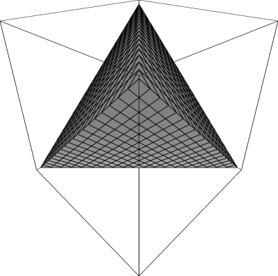
Figure 2: the tetrahedron

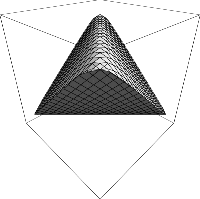
Figure 3: the “rounded tetrahedron”

The inequalities (12) imply that, as for the tetrahedron, the figure in (3b) has rectangular cross sections for fixed $\lambda_{3}$ with $|\lambda_{1}\pm\lambda_{2}|\leq\sqrt{(1+\lambda_{3})^{2}-t_{3}^{2}}$. When $t_{3}\neq 0$, the corners depend non-linearly on $\lambda_{3}$, yielding a curve of true extreme points. When $t_{3}=0$, the linearity in $\lambda_{3}$ yields a line segment so that we no longer have “true” extreme points.

The cases ${\bf t}=(\sqrt{1-\alpha^{2}},0,0)$ and ${\bf t}=(0,\sqrt{1-\alpha^{2}},0)$ are similar. The only difference is the orientation and displacement, e.g., whether the point [1,1,1] is replaced by $[\alpha^{2},\alpha,\alpha]$ or to $[\alpha,\alpha^{2},\alpha]$.

3.4 Channel capacity

The capacity of a quantum communication channel depends on the particular protocols allowed for transmission and measurement as well as the noise of the channel. See [3, 14] for definitions and discussion of some of these. We consider here only the so-called Holevo capacity that corresponds to communication using product signals and entangled measurements and is now believed (primarily on the basis of numerical evidence) to be the maximum capacity associated with communication that does not involve prior entanglements. The Holevo capacity is given by

$$C_{{\rm Holv}}(\Phi)=\sup_{\pi_{j},\,\rho_{j}}\left(S[\Phi(\rho)]-\sum_{j}\pi_{j}S[\Phi(\rho_{j})]\right),$$ (47)

where $S(P)=-\hbox{Tr}\,(P\,\log P)$ denotes the von Neumann entropy of the density matrix $P$, $\rho_{j}$ denotes a set of pure state density matrices, $\pi_{j}$ a discrete probability vector, and $\rho=\sum_{j}\pi_{j}\rho_{j}$. It is easy to see that for extreme points of the type (II) and (III), $C_{{\rm Holv}}(\Phi)=\log 2$ so that the capacity attains its maximal value, and for the completely noisy channel in (IC), $C_{{\rm Holv}}(\Phi)=0$.

By contrast, the non-unital situation (I) is more interesting because it includes channels for which the capacity (47)is strictly bigger than the classical Shannon capacity, i.e., the capacity for communication restricted to product input and measurements. Such channels demonstrate a definite quantum advantage. Moreover, the capacity is, in general, achieved neither with a pair of orthogonal input states, which would yield $h\big{(}\sin u\sin v)-h(\sqrt{1-\sin^{2}u\cos^{2}v}\big{)}$, nor with a pair of minimal entropy states, which would yield $h\big{(}\frac{\sin u}{\sin v}\big{)}$ where

$$h(t)=-\frac{1+t}{2}\log\frac{1+t}{2}-\frac{1-t}{2}\log\frac{1-t}{2}.$$ (48)

This behavior was observed first by Fuchs for a non-extreme channel [6]; subsequently, the amplitude-damping channel was studied by Schumacher and Westmoreland [27]. In both cases the work was numerical, but suggests that this situation is generic for channels that are translated orthogonal to the major axis of the ellipse.

In the case (IC) when the ellipsoid shrinks to a line, the capacity can be computed explicitly as

$$C_{{\rm Holv}}(\Phi) = h(\sqrt{t_{1}^{2}+t_{2}^{2}}=h(\cos u)$$

$$> \log 2-h(\sin u)$$

since $h(\cos\theta)+h(\sin\theta)\geq\log 2$. The expression $\log 2-h(\sin u)$ is the capacity of the unshifted channel. In this case, it is also the classical Shannon capacity. Holevo [8, 9] introduced such channels and showed that they suffice to demonstrate the “quantum advantage” mentioned above, although the both the minimal entropy and capacity are achieved with orthogonal inputs.

Remark: Holevo called channels of the form (IC) “binary” because their Kraus operators can be represented in the form $A_{1}=|e_{1}\rangle\langle\psi_{+}|,~{}A_{2}=|e_{2}\rangle\langle\psi_{-}|$ where the states $|e_{k}\rangle$ are orthonormal and $\psi_{\pm}$ can, in principle, be any pair of states, such as corresponding to $(\pm\cos x,\sin x)$. When $e_{1},e_{2}$ are the eigenvectors $\frac{1}{\sqrt{2}}(1,\pm 1)$ of $\sigma_{x}$, the resulting Kraus operators are

$$A_{1}=\frac{1}{\sqrt{2}}\pmatrix{\cos x&\sin x\cr\cos x&\sin x},~{}~{}A_{2}=\frac{1}{\sqrt{2}}\pmatrix{-\cos x&\sin x\cr\cos x&-\sin x}$$

One can easily check that this yields a map of type (IC) with $u=2x-\frac{\pi}{2},v={\textstyle\frac{1}{2}}\pi$ but the Kraus operators do not have the form (1.4).

Acknowledgment: It is a pleasure to thank Professor Chris King, Professor Denes Petz and Dr. Barbara Terhal for stimulating and helpful discussions, Dr. Christopher Fuchs for bringing reference [22] to our attention, and Professor Roger Horn for clarifying remarks about Lemma 8. After an earlier version of this paper [28] was posted we learned that Dr. Eleanor Rieffel and Dr. C. Zalka had independently obtained some similar results about the extreme points. We are grateful to them for a number of useful comments, including drawing our attention to Choi’s criterion for extremality which helped to streamline the proofs, and raising the question of the minimal number of extreme points needed for a given map. MBR would also like to thank Professor Ruedi Seiler for his hospitality at the Technische Universität Berlin, where part of this paper was written. The pictures were done with Mathematica and Adobe Illustrator. We want to thank Joachim Werner for his help in creating them.

References

- [1] A. Fujiwara and P. Algoet, “Affine parameterization of completely positive maps on a matrix algebra”, preprint. A. Fujiwara and P. Algoet, “One -to-one parameterization of quantum channels”, Phys Rev A, vol 59, 3290 –3294, 1999.
- [2] G.G. Amosov, A.S. Holevo, and R.F. Werner, “On Some Additivity Problems in Quantum Information Theory” preprint (lanl:quant-ph/0003002).
- [3] C. H. Bennett and P.W. Shor, “Quantum Information Theory” IEEE Trans. Info. Theory (1998).
- [4] M-D Choi, “Completely Positive Linear Maps on Complex Matrices” Lin. Alg. Appl. 10, 285–290 (1975).
- [5] M-D Choi, “A Schwarz Inequality for Positive Linear Maps on Algebras” Ill. J. Math. 18, 565–574 (1974).
- [6] C. Fuchs “Nonorthogonal quantum states maximize classical information capacity”, Phys. Rev. Lett 79 1162–1165 (1997). preprint (lanl: quant-ph/9703043)
- [7] R. Haag and D. Kastler, “ An Algebraic Approach to Quantum Field Theory”, J. Math. Phys. 5, 848–861 (1964).
- [8] A. S. Holevo, “On the capacity of quantum communication channel”, Probl. Peredachi Inform., 15, no. 4, 3-11 (1979) (English translation: Problems of Information Transm., 15, no. 4, 247-253 (1979)).
- [9] A. S. Holevo, ”Quantum coding theorems”, Russian Math. Surveys, 53(6), 1295-1331 (1999). quant-ph/9809023
- [10] R.A. Horn and C.R. Johnson, Matrix Analysis (Cambridge University press, 1985).
- [11] R.A. Horn and C.R. Johnson, Topics in Matrix Analysis (Cambridge University press, 1991).
- [12] M. Horodecki and P. Horodecki, “Reduction criterion of separability and limits for a class of protocols of entanglement distillation” xxx.lanl.gov preprint quant-ph/9708015.
- [13] C. King and M.B. Ruskai, “Minimal entropy of states emerging from noisy quantum channels” IEEE Trans. Info. Theory 47, 192–209 (2001).
- [14] C. King and M.B. Ruskai, “Capacity of Quantum Channels Using Product Measurements” J. Math. Phys. 42, 87–98 (2001)
- [15] K. Kraus, “General state changes in quantum theory” Ann. Physics 64, 311–335 (1971).
- [16] K. Kraus, States, Effects and Operations: Fundamental Notions of Quantum Theory (Springer-Verlag, 1983).
- [17] S.-H. Kye, “On the convex set of completely positive linear maps in matrix algebra,” Math. Proc. Camb. Phil. Soc. 122, 45–54 (1997).
- [18] E. Lieb and M.B. Ruskai “Some Operator Inequalities of the Schwarz Type” Adv. Math 12, 269–273 (1974).
- [19] G. Lindblad, “Completely Positive Maps and Entropy Inequalities” Commun. Math. Phys. 40, 147-151 (1975).
- [20] S. Lloyd, Science, 273, 1996, p. 1073.
- [21] M.A. Nielsen and I.L. Chuang, Quantum Computation and Quantum Information (Cambridge University Press, 2000).
- [22] Niu and Griffiths, “Two Qubit Copying Machine for Economical Quantum Eavesdropping” quant-ph/9810008
- [23] V. I. Paulsen, Completely bounded maps and dilations Pitman Research Notes in Mathematics Series, 146. (Longman Scientific and Technical, Harlow; John Wiley and Sons, Inc., New York, 1986).
- [24] G. Pedersen C*-algebras and their automorphism groups (Academic Press, 1979).
- [25] E. Rieffel and C. Zalka, private communications and unpublished manuscript.
- [26] B. M. Terhal, I. L. Chuang, D. P. DiVincenzo, M. Grassl, and J.A. Smolin, “Simulating quantum operations with mixed environments”, quant-ph/9806095.
- [27] B. Schumacher and M. D. Westmoreland, “Optimal signal ensembles” xxx.lanl.gov preprint quant-ph/9912122.
- [28] M.B. Ruskai S. Szarek and E. Werner xxx.lanl.gov preprint quant-ph/0005004