Stochastic Theory of Relativistic Particles Moving in a Quantum Field: I. Influence Functional and Langevin Equation

Abstract

We treat a relativistically moving particle interacting with a quantum field from an open system viewpoint of quantum field theory by the method of influence functionals or closed-time-path coarse-grained effective actions. The particle trajectory is not prescribed but is determined by the backreaction of the quantum field in a self-consistent way. Coarse-graining the quantum field imparts stochastic behavior in the particle trajectory. The formalism is set up here as a precursor to a first principles derivation of the Abraham-Lorentz-Dirac (ALD) equation from quantum field theory as the correct equation of motion valid in the semiclassical limit. This approach also discerns classical radiation reaction from quantum dissipation in the motion of a charged particle; only the latter is related to vacuum fluctuations in the quantum field by a fluctuation-dissipation relation, which we show to exist for nonequilibrim processes under this type of nonlinear coupling. This formalism leads naturally to a set of Langevin equations associated with a generalized ALD equation. These multiparticle stochastic differential equations feature local dissipation (for massless quantum fields), multiplicative noise, and nonlocal particle-particle correlations, interrelated in ways characteristic of nonlinear theories, through generalized fluctuation-dissipation relations.

I Introduction

A Particles and fields

Charged particles moving in a quantum field is an old topic in electromagnetic radiation theory, plasma physics and quantum/atom optics. Interesting features include the relation between quantum fluctuations and radiation reaction [1], and, for the case of uniformly accelerated detectors, thermal radiance in the detector (known as the Unruh effect [2]). For relativistic particles there are also bremsstrahlung, synchrotron radiation, and pair creation. The motion of congruences of charged particles shows up in particle beam, plasma and nuclear (e.g. heavy-ion collision) physics. Their collective or transport properties must be treated by additional statistical mechanical considerations beyond those applied to single particles.

Theoretically, since particle-field interaction is in principle described by quantum field theory, one may get the impression that ordinary field theoretic methods are both necessary and sufficient for the study of this problem. Quantum field theory, in the way we usually learn it, is customarily formulated in the context of, and with special emphasis on, how to answer questions posed in particle physics. For example, the S matrix is constructed for calculating scattering amplitudes, a perturbation expansion (e.g. Feynman diagram techniques) is used for theories with a small coupling constant (e.g., QED), and even the effective action is usually based on in-out (Schwinger-DeWitt) boundary conditions (the vacuum persistence amplitude). But, when one wants to find the evolution equation of a particle one needs an in-in boundary condition and an initial value formulation of quantum field theory [3, 4]. This is the starting point for constructing theories describing the nonequilibrium dynamics of many-particle systems [5] where both the statistical mechanics depicting the collective behavior of a congruence of particles as well as the statistical mechanical properties of interacting quantum field theory need to be included in our consideration [6, 7].

The relationship between the contrasting paradigms of particles and fields is at the heart of our inquiry. The concept of a particle is very different from that of a quantum field: a particle moving in real space cannot be completely described by, say, a number representation in Fock space, which underlies the second quantization formulation of canonical field theory. Background field decomposition into a classical field and its quantum fluctuations is a useful scheme, where one can follow the development of the classical background field with influences from the quantum fluctuations. While these methods have been applied extensively to the semiclassical evolution of quantum fields, the classical picture of particle motion is still quite remote. The Feynman path integral formulation (for particles worldlines as opposed to fields) makes it easier to introduce classical particle trajectories as the path giving the extremal contribution to the quantum action, the stationary phase defining one condition of classicality. One can then add on radiative corrections by carrying out the loop expansion. This approach puts a natural emphasis on particle trajectories rather than scattering amplitudes between momentum eigenstates. But how does one go further to incorporate or explain stochastic behavior of the particle? We shall see that when the coupling between the particle and the field is non-negligible, backreaction of the field (with all its activities such as vacuum polarization, pair creation, etc.) on the particle (beyond simple radiative corrections) imparts stochastic components to its classical trajectory.

At a deeper level, which we will tend to in the next series of papers, even a simple quest to understand the detailed behavior of quantum relativistic trajectories (i.e. worldlines) is a complex challenge, with problems connected with many central issues of quantum physics. For example, understanding how a particle moves through time (or more accurately, how a property that can be recognized as time emerges for a single particle) provides technical and conceptual insights into the larger questions concerning the nature of time in general. Here we focus on the regime where the notion of trajectory and particle identity is well-defined- this implies that both particle creation/annihilation and quantum exchange statistics (e.g. Fermi exclusion or Bose condensation effects) are of negligible importance.

Is there a unified framework to account for all these aspects of the problem? This is what we strive to develop in this series of papers. We see from the above cursory queries that to address this deceptively simple problem in its full complexity one cannot simply apply the standard textbook recipes of quantum field theory. Even a “simple” problem such as particles moving in a quantum field, when full backreaction is mandated, involves new ways of conceptualization and formulation. In terms of new conceptualization, it requires an understanding of the relation of quantum, stochastic, classical (as ingrained in the process of decoherence) behaviors, and of the manifestation of statistical mechanical properties of particles and fields, in addressing where dissipation and fluctuations arise and how the correlations of the quantum field enter. In terms of new formulation, it involves the adaptation of the open-systems concepts and techniques in nonequilibrium statistical mechanics, and an initial value (in-in) path integral formulation of quantum field (and quantized worldline) theory for deriving the evolution equations. We will discuss these two aspects to highlight the basic issues involved in this problem.

In this investigation we take a microscopic view, using quantum field theory as the starting point. This is in variance to, say, starting at the stochastic level with a phenomenological noise term often-times put in by hand in the Langevin equation. We want to give a first-principles derivation of moving particles interacting with a quantum field from an open-systems perspective. A consequence of coarse-graining the environment (quantum field) is the appearance of noise which is instrumental to the decoherence of the system and the emergence of a classical particle picture. At the semiclassical level, where a classical particle is treated self-consistently with backreaction from the quantum field, an equation of motion for the mean coordinates of the particle trajectory is obtained. This is identical in form to the classical equations of motion for the particle since higher-order quantum effects, which arise when there are nonlinear interactions, are suppressed by decoherence.

Backreaction of radiation emitted by the particle on the particle itself is called radiation reaction. For the special case of uniform acceleration it is equal to zero. This well-known, but at first-sight surprising, result is consistent owing to the interplay of the so-called acceleration field and radiation field [8]. Radiation reaction (RR) is often regarded as balanced by vacuum fluctuations (VF) via a fluctuation dissipation relation (FDR). This leads to a common misconception: RR exists already at the classical level, whereas VF is of quantum nature. There is, as we shall see in this paper, nonetheless a FDR at work balancing quantum dissipation (the part which is over and above the classical radiation reaction) and vacuum fluctuations. But it first appears only at the stochastic-level, when self consistent backreaction of the fluctuations in the quantum field is included in our consideration. In addition to providing a source for decoherence in the quantum system making it possible to give a classical description such as particle trajectories, fluctuations in the quantum field are also responsible for the added dissipation (beyond the classical RR), and a stochastic component in the particle trajectory (beyond the mean). Their balance is embodied in a set of generalized fluctuation-dissipation relations, the precise conditions for their existence we will demonstrate in this paper.

Ultimately a satisfactory description of the particle-field system would have to come from a full quantum theory treatment. One needs to stipulate and demonstrate clearly what successive approximations one introduces to some larger interacting quantum system will enable us to begin to see the precursor or progenitor of the particle, and the residual or background quantum field, depicted so simply in the end as the particle-field system in the conventional field theory idiom. The imprint of the particle’s motion is left in the altered correlations of the quantum field [9].

Later we shall see that while the problem of the nonequilibrium quantum dynamics of relativistic particles (or fields) is important in its own right; the rich physics contained is also closely connected with other problems of fundamental significance such as Quantum Gravity and String theory, including semiclassical gravity and quantum fields in black hole and early universe spacetimes. The remainder of this introduction summarizes the main ideas in this work and places it in the diverse range of prior research on this subject matter. We try to present a viewpoint and method which may provide a comprehensive and unified account while pointing out specific areas requiring further attention.

B Quantum, Stochastic and Semiclassical Regimes

Our treatment in this first series emphasizes the semiclassical level and stochastic regimes. Our approach is sharply distinguished from the case where the motion of the particle is prescribed, i.e., a stipulated trajectory, that is characteristic of many treatments of ‘particle-detectors’ in quantum fields. Here, the trajectory is determined by the quantum field in a self-consistent manner. In the former case, there is a tacit presence of an agent which supplies the energy to keep the trajectory on a prescribed course, its effect showing up in the radiation given off by a detector/particle undergoing, say, acceleration. The field configuration would have to adjust to this prescribed particle motion accordingly, without affecting the particle motion. In the latter case, the only source of energy sustaining the particle’s motion arises from the quantum field, and both the field and particle adjust to each other in a self-consistent manner. The former case has been treated in detail by Raval, Hu, and Anglin (RHA) [9] (see references therein for prior work) using the concept of quantum open-systems and the influence functional technique. We investigate the second class of problems now with the same open-system methodology.

A closed quantum system can be partitioned into several subsystems according to the relevant physical scales. If one is interested in the details of one such subsystem, call it the distinguished (relevant) system, and decides to ignore certain details of the other subsystems, comprising the environment, the distinguished subsystem is thereby rendered as an open-system [10]. The overall effect of the coarse-grained environment on the open-system can be captured by the influence functional technique of Feynman and Vernon [11], or the closely related closed-time-path effective action method of Schwinger and Keldysh [3]. These are initial value formulations. For the model of particle-field interactions we study, this approach yields an exact, nonlocal, coarse-grained effective action (CGEA) for the particle motion [12]. The CGEA may be used to treat the complete quantum dynamics of interacting particles. However, only when the particle trajectory becomes largely well-defined (with some degree of stochasticity caused by noise) as a result of effective decoherence due to interactions with the field can the CGEA be meaningfully transcribed into a stochastic effective action, describing stochastic particle motion [9, 13, 14].

The effect of the environment (the coarse-grained subsystems) on the system (the distinguished subsystem) is known as backreaction. One form of classical backreaction in the context of a moving charged particle in a quantum field is radiation reaction which exerts a damping effect on the particle motion. As remarked before, it should not be mistaken to be balanced directly by an FDR with vacuum fluctuations of the quantum field. The latter induce quantum dissipation and are instrumental to decohering the classical particle. Let us now further examine the role of dissipation, fluctuations, noise, decoherence [6, 7] and the relation between quantum, stochastic and classical behavior [13, 14].

Decoherence or dephasing refers to the loss of phase coherence in the quantum open system arising from the interaction of the systems with the environment. Effective decoherence brings about the emergence of classical behavior in the system which generally carries also stochastic features. Under certain conditions quantum fluctuations in the environment act effectively as a classical stochastic source, or noise. While noise in the environment is instrumental in decoherence, decoherence is a necessary condition for the appearance of a classical trajectory. In this emergent picture of the quantum to classical transition, there is always some degree of resultant stochasticity in the system dynamics [13]. When sufficiently coarse-grained descriptions of the microscopic degrees of freedom are considered, nearly complete decoherence leads to negligible noise, and the classical description of the world is complete. Moving back from classicality towards a description of more finely-grained histories, the quantum effects suppressed by decoherence on macroscopic scales reveal themselves in the emergence of stochasticity. In this realm, decoherence, noise, dissipation, particle creation, and backreaction are seen as aspects of the same basic quantum-open-system processes [13, 14]. If ‘minimal’ additional smearing is not adequate to decohere the particle trajectories, the stochastic limit is not physically meaningful because the quantum interference between particle histories continues to play a significant role. Even without a field’s presence as an environment, the particle’s own quantum fluctuations (represented by its higher order correlation functions) may be treated as an effective environment for the lower-order particle correlation functions (particularly the mean trajectories), so that a stochastic regime may still be realized when appropriately coarse-grained histories are considered [6, 7, 14]. When averaged descriptions are considered such that the coarse-grained set of histories has substantial inertia, the quantum-fluctuation induced noise is negligible, and one moves from the stochastic to semiclassical domains. Note that there is now growing recognition that the transition from quantum to classical behavior [13, 15] is characterized by a rich diversity of scales and phenomena, and it should therefore not be thought of as a single transition, but rather a succession of regimes that may, or may not, be well-separated in practice [16, 17].

The view of the emergence of semiclassical solutions as decoherent histories [13] also suggests a new way to look at the radiation-reaction problem for charged particles. The classical equations of motion with backreaction are known as the Abraham-Lorentz-Dirac (ALD) equations [18]. The solutions to the ALD equations have prompted a long history of controversy due to such puzzling features as pre-accelerations, runaways, non-uniqueness of solutions, and the need for non-Newtonian initial data [8]. It has long been felt that the resolution of these problems must lie in quantum theory. But, this still leaves open the questions of when, if ever, the Abraham-Lorentz-Dirac equation appropriately characterizes the classical limit of particle backreaction; how the classical limit emerges; and what imprints the correlations of the quantum field environment leave. We show that these questions, and the traditional paradoxes, both technical and conceptual, can be resolved in the context of the initial value quantum open system approach.

Indeed, since every possible fine-grained history is included in the path integral for the quantum evolution, there is no a priori reason to reject fine-grained runaway solutions as unphysical, nor is there any sense in which a particular fine-grained history pre-accelerates, since the fine-grained paths that appear in the path integral aren’t causally determined by earlier events in any case. From this perspective, the appropriate questions to address are, which ‘quasi-classical’ coarse-grained solutions decohere more readily. Certainly it would be strange if runaway (or pre-accelerating) decoherent coarse-grained histories occurred with any appreciable associated probability. So the question that should be asked, in the context of how classical solutions arise from the quantum realm, is whether decohered particle-histories are 1) solutions to the ALD equation, 2) unique and runaway free, and 3) without preacceleration on scales larger than the coarse-graining scale at which the trajectories decohere. We shall see that, in fact, the semiclassical solutions do satisfy these criteria, and therefore, one is entirely justified in using the ALD equation in the classical limit. One also sees that because this approach describes coarse-grained histories, the ALD equation as an approximation fails in the finest-grained quantum limit.

Therefore, a fundamental understanding of the stochastic and semiclassical limits must be set in the context of the full quantum theory of particles and fields. In the second series of papers, we further develop the worldline plus field framework to describe fully quantized relativistic particles in motion through spacetime interacting with quantum fields and highlight its semiclassical, stochastic and quantum features. This framework for understanding relativistic systems is important because, in the nonequilibrium dynamics of real particles, the localized nature of the particle state is a prominent characteristic of the semiclassical limit, and this fact is not most naturally described by the usual perturbative field theory in momentum space. Furthermore, interaction, correlation, measurement and decoherence invariably take place in both space and time. The incorrect treatment of “measurement” as an instantaneous occurrence leads to fundamental inconsistencies in the description of physical initial states which continues to be a substantial obstacle to a deeper understanding of decoherence and nonlocal correlation. For this reason, addressing the stochastic (and quantum) limits in a relativistic framework treating space and time covariantly is a vital element in fully understanding the stochastic-semiclassical limit. By developing a new framework for relativistic particle-field quantum dynamics we will show how this alternative approach provides powerful tools for addressing both conventional issues, and for exploring new questions.

C Coarse-graining the particle

Our problem, as well as many others from quantum and atom optics, provides a good example of where a quantum field (e.g. photons) acts as an environment in its influence on an atom or electron system. There are, of course, physical contexts for which it is more appropriate to coarse-grain the particle degrees of freedom, whereby one obtains a coarse-grained effective action for the field. In this complementary view, matter plays the role of an environment for the field as a system. When both particle and field coarse-grainings converge to mutually decoherent sets of particle and field histories, one recovers the classical limit [19]. These regimes are illustrated schematically in Figure 1, where the field degrees of freedom are denoted by $\varphi,$ and the particle degrees of freedom are denoted by $z.$

D Nonlinear Coupling

Comparing with prior work on this subject matter using the same approach, the most closely related being that of Raval, Hu and Anglin [9], who derived the influence functional for n-detectors moving in a quantum field, the main distinct feature here is that the particle trajectory is not prescribed, but is a dynamical degree of freedom determined self-consistently by the field. As such the coupling between the particle(s) and the field is of a more fundamental nonlinear nature. One type of nonlinear coupling between the system and the environment in the quantum Brownian motion models [20, 21, 22] has been considered by Hu, Paz, and Zhang [21]. Their model contains nonlinear couplings that are polynomial in the field variables, whereas here we consider the opposite example, where the field variables are linear, but the system variables are not. This is the case for QED, which is our ultimate goal (to be discussed in Paper III [23] of this series).

Our treatment of nonlinear particle-field interactions is in sharp contrast with the existing body of work on the semiclassical and stochastic limit for linear QBM. We find that the requirement of self-consistency, together with the nonlinearity of the fundamental interactions, leads to a description of the stochastic limit that is more unified and tightly constrained than that which has been described up to now. In fact, confronting nonlinear systems is a crucial next step in exploring the stochastic limit, and the deeper relationship between noise, decoherence, and the intricate evolution of correlations for systems with many degrees of freedom. Most studies of decoherence have invoked linear systems with an (externally) predetermined basis of states which are then shown to decohere. But a complete description of decoherence must include the mechanism by which a decoherent basis of states is self-consistently (e.g. not externally) selected. Understanding this mechanism as a dynamical feature of nonlinear theories is an important problem that cannot be fully addressed within linear models.

Another important difference between linear and nonlinear theories is in their respective equations of motion for correlation functions. For linear theories, these are just given by the classical equations of motion, and the quantum evolution may be reproduced by a probabilistic description of initial conditions. An example of this is the Wigner function evolution for linear systems with initially positive definite distributions in phase spaces. The equations of motion are then the classical ones, and negative values of the Wigner function never evolve in the future. One may then view the theory as dynamically equivalent to classical statistical dynamics (though of course the meaning of the Wigner functions is still quantum [24]). This fact is what makes the construction of a stochastic limit that bridges linear classical and quantum theories fairly straightforward. The same is not true of nonlinear theories. Their quantum equations of motion (even for the mean-field) are not equivalent to the classical ones. This implies that there are important qualitative differences in the quantum dynamics of linear versus nonlinear theories that are significant even in the semiclassical regime, and that will be missed by the study of linear systems alone.

The important result in this first paper is the derivation of self-consistent Langevin equations for relativistic particle motion in a quantum field starting from relativistic quantum mechanics. A stochastic description of the limit of nonlinear theories requires great care, and, in its most general form, will involve nonlinear stochastic differential equations where the statistics of the induced particle fluctuations are externally determined by the quantum statistics of the fields.

Because there are inherent dangers in a phenomenological approach to nonlinear stochastic equations, it is crucial to work from first principles stressing the microscopic origin of fluctuations. In this work, we treat an example of a nonlinear stochastic system in the regime where decoherence allows the expansion around the semiclassical solution. The decoherent semiclassical solutions need not, and usually are not, equilibrium solutions. Hence, compared with the traditional derivation of the Langevin equations in the context of near-equilibrium linear response theory, this method is significantly more general.

For Langevin equations the effect of the field is registered in the stochastic properties of the particles. The stochastic mean of the equations of motion corresponds to the mean-field semi-classical limit; but in addition, the symmetrized n-point correlation functions for the particles are given by the higher order stochastic moments. Therefore, the stochastic particles may be thought of as being “dressed” by the non-local statistics of the field. These equations impart stochastic features to the particle and field properties beyond the semiclassical limit, leading towards the quantum domain. The stochastic equations of motion featuring nonlocal noise, causal particle-particle interactions, and nonlocal particle-particle correlations make the evolution highly non-Markovian (i.e. history dependent). Only in the single particle semiclassical limit (with local dissipation and white noise) is the evolution strictly Markovian. For well separated particles, in the high temperature limit, the Langevin equations may be approximated by Markovian dynamics; this is the regime in which the nonlocal role of the quantum vacuum has been essentially washed out. But as one moves more deeply into the stochastic regime (especially at low temperatures), the Markovian approximation is no longer adequate. It is in this realm that our methods are markedly distinct from the Hamiltonian methods more commonly used in the derivation of Markovian master equations.

E Prior work in relation to ours

The treatment of a quantum field as a bath of harmonic oscillators has a long history. Many authors take a semi-phenomenological approach in adding a noise to the quantum equation of motion by hand to get the Quantum Langevin equations (QLE). This practice works reasonably well in the linear response regime for a system in equilibrium, but can otherwise violate the fluctuation-dissipation relation and bring about pathologies (such as a-causal evolution). There are many ways to derive the QLE describing the dissipative dynamics of a quantum system in contact with a quantum environment, such as modified (Heisenberg picture) Hamilton equations of motion or path integrals. Caldeira and Leggett’s revival of the Feynman-Vernon influence functional in the study of quantum Brownian motion (QBM) has led to an extensive literature on QBM [20], particularly in regard to decoherence [21, 25].

Ford, Lewis, and O’Connell have done systematic and comprehensive work on the problem of charge motion in an electromagnetic field as a thermal bath in the linear (dipole coupling) regime [26]. They have detailed the conditions for causality and a good thermodynamic limit, and have further used the QLE paradigm to find stochastic equations of motion for non-relativistic charged particles in the equilibrium limit. A crucial point of their analysis is that the solutions can be (depending on the cutoff of the field spectral density) runaway free and causal in the late-time limit [27]. In [28], they suggest a form of the equations of motion that give fluctuations without dissipation for a free electron, but this result arises from the particular choice they made of a field cutoff. In contrast, we take the effective theory point of view which emphasizes the typical insensitivity of low-energy phenomena to unobserved high-energy structure. The following two papers in this series make clear that a special value for the cutoff is unnecessary for consistency of the low-energy behavior. Further distinctions are briefed as follows: First, our general method extends to the nonequilibrium regime, allowing consideration of specific initial states at a finite time in the past. Second, we do not make the dipole approximation ab initio because we are especially interested in the nonequilibrium dynamics of nonlinear systems. When our equations of motion are linearized, we pay special attention to the constraints that the original nonlinear theory imposes. Third, by adopting the worldline quantization framework, we are able to derive equations of motion from fully relativistic quantum mechanics. Fourth, we highlight the role of decoherence in the emergence of a stochastic regime. Fifth, we show how nonlocality may still be a feature in the stochastic regime, unless sufficient noise washes out the nonlocal correlations between separate particles.

Our results also represent an extension of Barone and Caldeira’s analysis of decoherence for an electron in an quantum electromagnetic field [30]. Their work employs the path integral method except they are limited to non-relativistic particles and dipole coupling, and it focuses mainly on the reduced density matrix. Rather we give a full description of the stochastic dynamics of this nonlocal nonlinear theory. An advantage of Barone and Caldeira’s work is that it is not limited to initially factorized states; they use the preparation functional method which allows the inclusion of initial particle field correlations. Despite this, Romero and Paz have pointed out that the preparation function method still suffers from an unphysical depiction of the initial state [31]. For this reason, a completely satisfactory treatment of particle decoherence in a field-environment that accounts for particle-field correlations in more realistic (i.e. physically prepared) states remains to be given.

Using the influence functional, Diósi [32] derives a Markovian master equation in non-relativistic quantum mechanics. In contrast, it is our intent to emphasize the non-Markovian and nonequilibrium regimes with special attention paid to self-consistency. The work of [32] differs from ours in the treatment of the influence functional as a functional of particle trajectories in the relativistic worldline quantization framework. Ford has considered the loss of electron coherence from vacuum fluctuation induced noise with the same noise kernel that we employ [33]. However, his application concerns the case of fixed or predetermined trajectories.

F Organization, notations and units

In Section 2, we begin with a review on how a quantum field can be treated as a bath of harmonic oscillators and we connect with the well-studied quantum Brownian motion model (QBM) and quantum Langevin equations (QLE) [11, 20, 21, 26, 30, 34, 35]. We write down the form of the influence functional (IF) for nonlinear particle-field interactions, and we further review the influence functional formalism in Appendix A, where we discuss the necessary assumptions for deriving an evolution propagator for the kind of hybrid particle/field model that we employ. Underlying the formulation in Appendix A is the worldline quantization method for relativistic particles where the particle coordinate is the relevant particle degree of freedom. Use of this framework, rather than the conventional quantum field description for the charged particles, is central to this work. However, the detailed development of this approach is not needed for the semiclassical and stochastic regimes considered in this first series.

In Sec. 3, we derive the coarse-grained effective action (CGEA). The background material in our approach consists of the Schwinger-Keldysh closed-time-path (CTP) effective action applied to an open system, which results in a CTP CGEA that is closely related to the influence action in the Feynman-Vernon influence functional method. For easy access and identification of notations and conventions, we review these necessary formalisms in the Appendices, which can be read independently. These techniques provide a general and powerful framework for studying nonequilibrium quantum processes, especially for non-Markovian dynamics, which are prevalent when backreaction of the environment on the system is fully and correctly accounted for. We introduce the reduced-density-matrix for a system after assuming a system-environment partition. The reduced density matrix evolution operator is found in terms of the IF, and the CGEA. In Sec. 4, we define the stochastic effective action, and show the close relationship of noise, dissipation, and decoherence in the stochastic limit. In Sec. 5, we discuss stochastic fields. Sec. 6 presents a general (i.e., not restricted to a specific model of the particles or field) derivation of the stochastic equations in the form of nonlinear Langevin equations for general nonlinear particle-field coupling. We discuss when the traditional linear Langevin equations may be recovered. In Sec. 7 we derive a generalized fluctuation-dissipation relation for the noise and radiation-reaction in these expressions. This provides the necessary framework of a stochastic theory approach to investigate relativistic particle motion in quantum fields.

In Paper II [29], we shall apply these results to a specific model of relativistic particles in a scalar field. We derive the influence functional and stochastic effective action for this nonlinear model, and then discuss in detail the semiclassical limit. The main result is the derivation of equations of motion for the semiclassical limit that, to lowest order, are modified (time-dependent) Abraham-Lorentz-Dirac (ALD) equations for charged-particle radiation reaction. This work demonstrates that the ALD equation is a good approximation to the semiclassical limit of scalar QED, in the regime where the particles are effectively classical. This derivation is more general, however, and reveals the time-dependent renormalization and radiation-reaction typical of nonequilibrium quantum field theory. These features play a crucial role in establishing the consistency of this limit by showing that runaway solutions and acausal effects do not occur when the field is suitably regulated. We then derive (time-dependent) Abraham-Lorentz–Dirac-Langevin (ALDL) equations, which describe the fluctuations (and radiation reaction) of relativistic particles in the stochastic limit. We use these results to explore the question of Brownian motion for a free particle in a quantum scalar field.

In Paper III [23], we extend these results to the electromagnetic field by deriving the influence functional for QED in the Lorentz gauge, from which we find the interacting photon-particle stochastic action. In the semiclassical limit we obtain a modified, time-dependent, ALD solution for QED. We then demonstrate a direction dependent Unruh effect with the vacuum fluctuations of the field appearing thermal (at the Unruh temperature) for charged particles in a constant electric field. This general approach clearly illustrates the distinct natures of ALD radiation reaction, the associated ordinary radiation into infinity, and the Unruh effect, while at the same time deriving all these effects in a unified and self-consistent manner. As an interesting application, the Langevin equation may be viewed as a model for a stochastic particle event horizon, with implications for a nonequilibrium treatment of black hole Hawking radiation and horizon fluctuations.

Our second series of papers (IV and V [36]) will be on relativistic quantum particle-field interaction. It is here that the pre-cursors of the quantized worldline framework introduced in Appendix A are fully developed. In Paper IV, we ‘first’ quantize the free relativistic particle using the path integral method. The worldline path integral representation is used to construct the “in-out” and “in-in” relativistic particle generating functional for worldline coordinate correlation functions. In Paper V, we use the influence functional to construct an interacting quantum theory of both relativistic particles and fields. This involves the introduction of a nonlocal worldline kernel that provides a route for exploring the role of correlation, dissipation, and nonequilibrium open-system phenomena in particle creation and other relativistic processes. This work is also a model for how open-system methodology may be introduced into String theory since the worldline path integral is the point particle limit of the String case. This formalism provides a powerful approach to a new set of quantum-relativistic-statistical processes where one may simultaneously take advantage of the influence functional and first-quantization (worldline) techniques.

We shall usually set $c=1$, but keep $\hbar$ explicit as a marker for quantum effects. The metric tensor $g_{\mu\nu}$ is diag$(+1,-1,-1,-1)$. Greek letters will (usually) denote spacetime indices, and Latin letters $a,b,c$ will indicate the CTP time-branch (see Appendix C). The mixed function/functional notation $f[z;x)$ will be used when $f$ is a functional of $z,$ but a function of $x.$ The Einstein summation convention is employed except when otherwise noted. Particle degrees of freedom will be collectively denoted $z=\left\{z_{n}^{\mu}\left(\tau_{n}\right)\right\}$ with $\tau_{n}$ as their worldline parameters. The path integral measures are denoted $Dz$ and $D\varphi,$ and are defined in Appendix A.

II The effective action, effective field theory, and particle reduced density-matrix

Particles moving in quantum fields may be cast in the form of nonlinear quantum Brownian motion. In this paper, a set of $N$ particles (with action $S_{z})$ constitutes the system and a scalar field $\hat{\varphi}\left(x\right)$ (with the action $S_{\varphi})$ constitutes the environment. The particles and field interact nonlinearly as determined by an interaction action $S_{int}.$ The n^th particle degree of freedom is its spacetime trajectories $z_{n}^{\mu}\left(\tau_{n}\right)$ parametrized by $\tau_{n}$, which is not necessarily the particle’s proper time. In this first series, our focus is on the stochastic dynamics of the particle worldlines; for simplicity, we neglect additional particle degrees of freedom such as spin. We also work in the regime where particles have approximately well-defined (emergent) trajectories, though with statistical fluctuations arising from the particles’ contact with the quantum field. Consequently, the forces that arise from spin-statistics (e.g. Fermi-exclusion or Bose-condensation) are negligible. We discuss how these quantum effects are suppressed by decoherence (the same decoherence that gives the particles stochastic trajectories) in our second series.

In this relativistic treatment, both the particle’s space and time coordinates will emerge as stochastic processes, with correlation functions of the form $\langle z_{1}^{\mu}\left(\tau_{1}\right)...z_{N}^{\nu}\left(\tau_{N}\right)\rangle_{s}.$ The notation $\langle\rangle_{s}$ denotes the stochastic average with respect to a derived probability distribution. The statistics of these processes are found from the underlying quantum statistics of the quantum field acting as an environment. The semiclassical regime is characterized by the particle trajectories being well-defined classical variables. The stochastic regime is intermediate between the semiclassical and quantum regimes, where the particle worldlines are classical stochastic processes.

The quantum open-system of particle degrees of freedom is described by the reduced density-matrix

$$\hat{\rho}_{r}\left(t\right)=Tr_{\varphi}\hat{\rho}_{U}\left(t\right),$$ (1)

where $\hat{p}_{U}\left(t\right)$ is the unitarily evolving state of the universe (i.e. the particles plus field) at time $t.$ We assume that the initial state (at time $t_{i})$ of the universe can be represented in the factorized (tensor-product) form

$$\hat{\rho}_{U}\left(t_{i}\right) =\hat{\rho}_{z}\left(t_{i}\right)\otimes\hat{\rho}_{\varphi}\left(t_{i}\right)$$ (2)

$$=\int d\varphi_{i}d\varphi_{i}^{\prime}d{\bf z}_{i}d{\bf z}_{i}^{\prime}\rho_{\varphi}\left(\varphi_{i},\varphi_{i}^{\prime}\right)$$ (3)

$$\times\rho_{z}\left(z_{i},z_{i}^{\prime}\right)|\varphi_{i},z_{i}\rangle\langle\varphi_{i}^{\prime},z_{i}^{\prime}|,$$ (4)

where $\hat{\rho}_{z}$ and $\hat{\rho}_{\varphi}$ have been expanded in terms of basis states $|\varphi_{i},z_{i}\rangle=|\varphi_{i}\rangle\otimes|{\bf z}_{i},t_{i}\rangle.$ The initial particles states are the Lorentz invariant relativistic configuration-space state defined as

$$|z_{i}\rangle \equiv|{\bf z}_{i},t_{i}\rangle$$ (5)

$$=\int\frac{d^{4}p}{\left(2\pi\right)^{4}}\delta^{\left(4\right)}\left(p^{2}-m^{2}\right)\theta\left(p^{0}\right)e^{\frac{i}{\hslash}p_{\mu}z^{\mu}}|p\rangle,$$ (6)

where we have assumed that the initial particle state is positive frequency (this assumption may be relaxed).

The particle’s reduced density-matrix at later times is given by (see Appendix A)

$$\rho_{r}\left(z_{f},z_{f}^{\prime}\right) =\int d{\bf z}_{i}d{\bf z}_{i}^{\prime}J_{r}\left(z_{f},z_{f}^{\prime};z_{i},z_{i}^{\prime}\right)$$ (7)

$$\times\rho_{z}\left(z_{i},z_{i}^{\prime}\right).$$ (8)

The variable $z$ stands for the entire collection of particle coordinates $\left\{z_{n}^{\mu}\right\}.$ The open-system evolution operator $J_{r}$ is given by

$$J_{r}\left(z_{f},z_{f}^{\prime};z_{i},z_{i}^{\prime}\right) =\int_{{\bf z}_{i},{\bf z}_{i}^{\prime}}^{{\bf z}_{f},{\bf z}_{f}^{\prime}}DzDz^{\prime}e^{\frac{i}{\hslash}\left(S_{z}\left[z\right]-S_{z}\left[z^{\prime}\right]\right)}$$ (9)

$$\times F\left[z,z^{\prime}\right].$$ (10)

$F\left[z,z^{\prime}\right]$ is the influence functional introduced by Feynman and Vernon [11]. The measure $Dz$ depends on the details of how the particle action is defined and quantized, and it may implicitly include additional gauge degrees of freedom (such as a lapse variable $N$). In the semiclassical/stochastic treatment presented in this paper, we will in fact assume that the particle degrees of freedom have been gauge-fixed so that the parameters $\tau$ are the proper-times. The detailed treatment of the influence functional for relativistic particle worldlines is found in our second series [36], though a brief discussion may be found in Appendix A and in paper III [23].

The influence functional is given by

$$F\left[z,z^{\prime}\right] =\int d\varphi_{f}d\varphi_{i}d\varphi_{i}^{\prime}\int_{\varphi_{i},\varphi_{i}^{\prime}}^{\varphi_{f}=\varphi_{f}^{\prime}}D\varphi D\varphi^{\prime}$$ (11)

$$\times e^{\frac{i}{\hslash}\left(S_{\varphi}\left[\varphi\right]-S_{\varphi}\left[\varphi^{\prime}\right]+S_{int}\left[\varphi,z\right]-S_{int}\left[\varphi^{\prime},z^{\prime}\right]\right)}$$ (12)

$$\times\rho_{\varphi}\left(\varphi_{i},\varphi_{i}^{\prime};t_{i}\right)$$ (13)

$$=\exp\left\{\frac{i}{\hslash}S_{IF}\left[z.z^{\prime}\right]\right\},$$ (14)

where $S_{IF}\left[z,z^{\prime}\right]$ is called the influence action. Notice that the definition of the influence functional itself involves only path integrals over the fields $\varphi,$ and hence, does not require doing particle worldline path integrals. Indeed, the results of this paper follow from effectively treating the worldlines as classical variables coupled to a quantum field, which is the usual semiclassical paradigm. In the next section we indicate the connection between the worldlines as classical variables and the quantum equations of motion for the quantum-average trajectories.

Defining the coarse-grained effective action

$$S_{CGEA}=S_{z}\left[z\right]-S_{z}\left[z^{\prime}\right]+S_{IF}\left[z,z^{\prime}\right],$$ (15)

$J_{r}$ may, alternatively, be expressed as

$$J_{r}\left(z_{f},z_{f}^{\prime};z_{i},z\right)=\int_{{\bf z}_{i},{\bf z}_{i}^{\prime}}^{{\bf z}_{f},{\bf z}_{f}^{\prime}}DzDz^{\prime}e^{\frac{i}{\hslash}S_{CGEA}\left[z,z^{\prime}\right]}.$$ (16)

The evolution kernel $J_{r}$ gives all information about the quantum open-system dynamics of the particles.

If the particle-field interaction is characterized by a coupling constant $e$ and is linear in the field variables, the influence action is of order $e^{2}.$ One approximation scheme for Eq. (16) is to expand the influence functional as

$$e^{\frac{i}{\hslash}S_{IF}\left[z,z^{\prime}\right]}=1+\frac{i}{\hslash}S_{IF}\left[z,z^{\prime}\right]+{\cal O}\left(e^{4}\right),$$ (17)

giving a perturbation theory based on the order of a coupling constant. $J_{r}$ then describes free quantized-particle evolution punctuated by discrete interactions with the field. This is just ordinary perturbative quantum field theory in the “in-in” formulation. Unlike “in-out” field theory, the lowest order (non-trivial) terms are of order $e^{2},$ which is natural since $J_{r}$ gives the evolution of the density matrix, not the wavefunction. But, particularly when there is a background field $\bar{\varphi}=\langle\hat{\varphi}\rangle,$ (17) does not give an accurate depiction of the classical limit of particle trajectories, say, as given by the mean-values $\langle\hat{z}_{n}\rangle=\bar{z}$, where $\hat{z}_{n}$ is the quantum operator for the particle’s coordinates. The infinite set of background field terms in the expansion from (17) may be summed, giving a far more accurate approximation to the particle evolution. The resulting re-organization of Feynman diagrams is automatically obtained by performing a saddle point expansion of (16).

It is convenient to define sum and difference variables

$$z^{-} =\left(z-z^{\prime}\right)$$ (18)

$$z^{+} =\left(z+z^{\prime}\right)/2.$$ (19)

Evaluating the evolution kernel in Eq. (16) for linear systems is a standard step in the derivation of the master equation using path integral methods. One begins by reparametrizing the worldlines defining the fluctuation and classical worldlines, $\breve{z}_{n}$ and $\bar{z}_{n},$ respectively, by

$$\breve{z}_{n}^{\pm}=\hat{z}_{n}^{\pm}-\bar{z}_{n}^{\pm},$$ (20)

The extremal solutions to the effective action, denoted $\bar{z}_{n},$ are defined to be the classical solutions to the real part of $S_{CGEA}\left[z^{\pm}\right]:$

$$\left.\frac{\delta S_{CGEA}^{R}\left[z^{\pm}\right]}{\delta z_{n}^{\pm}}\right|_{z^{\pm}=\bar{z}_{n}^{\pm}}=0,$$ (21)

satisfying the boundary conditions

$${\bf\bar{z}}^{\pm}(t_{i})={\bf z}_{i}^{\pm}$$ (22)

This definition is made because the imaginary part of the effective action does not modify the stationary phase solution.

The evolution operator for the open system is then given by

$$J_{r}\left(z_{f}^{\pm},z_{i}^{\pm}\right)=e^{\frac{i}{\hslash}S_{CGEA}^{R}\left[\bar{z}^{\pm}\right]}\int_{{\bf\breve{z}}_{i}^{\pm}=0}^{{\bf\breve{z}}_{f}^{\pm}=0}D\breve{z}^{\pm}$$ (23)

$$\times e^{\frac{i}{\hslash}\int d\tau\frac{\delta S_{CGEA}^{I}}{\delta\bar{z}^{a}\left(\tau\right)}\breve{z}^{a}\left(\tau\right)+\frac{i}{2\hslash}\int\int d\tau d\tau^{\prime}\frac{\delta^{2}S_{CGEA}}{\delta\bar{z}^{a}\delta\bar{z}^{b}}\breve{z}^{a}\left(\tau\right)\breve{z}^{b}\left(\tau^{\prime}\right)}$$ (24)

$$\times\left(1+{\cal O(}\breve{z}^{3}\right)),$$ (25)

where we have factored out the “zero-loop” term in front, and expanded the exponential of the non-quadratic terms in the effective action. $S_{CGEA}^{I}$ is the imaginary part of the effective action.

The higher-order quantum corrections depend on the solutions $\bar{z}_{n}^{\pm}$ unless the effective action is quadratic; and hence, the model is purely linear. For the linear case, $J_{r}$ may be found exactly since all the path integrals are Gaussian. It is given by

$$J_{r}\left(z_{f}^{\pm};z_{i}^{\pm}\right)=F\left(t_{f},t_{i}\right)\times e^{\frac{i}{\hslash}S_{CGEA}\left[\bar{z}^{\pm}\right]}$$ (26)

where $F$ may be found by the normalization condition

$$\int dz_{f}dz_{f}^{\prime}\delta(z_{f}-z_{f}^{\prime})\left.J_{r}\left(z_{f},z_{f}^{\prime};{\bf z}_{i}^{\pm},t_{i}\right)\right|_{t_{f}=t_{f}^{\prime}}$$ (27)

$$=\delta\left(z_{i}-z_{i}^{\prime}\right).$$ (28)

From $J_{r}$ it is straightforward to find the master equation from the expression

$$\frac{\partial}{\partial t_{f}}\rho_{r}\left(z_{f}^{\pm}\right)=\int d{\bf z}_{i}^{+}d{\bf z}_{i}^{-}\frac{\partial}{\partial t_{f}}J_{r}\left(z_{f}^{\pm};z_{i}^{\pm}\right)\rho_{r}\left(z_{i}^{\pm}\right).$$ (29)

Because the one-loop (fluctuation) term is independent of $\bar{z}$ for linear theories, the resulting noise and dissipation are independent of the system history. It is only for linear theories that the noise induced by the environment is completely extrinsic in this sense.

For non-linear theories, the one-loop (and higher-order) corrections will depend on $\bar{z}^{\pm}$ and hence will modify the master equation, giving system-history dependent (colored) noise and dissipation. But, rather than using the master equation as our primary tool, we instead follow the approach in [9, 37] for deriving quantum Langevin equations [11], to find a stochastic description of the particle dynamics from the influence functional.

III Influence functional for quantum scalar field environment

We now derive the influence functional assuming a system of spinless particles locally coupled to a scalar field. The free scalar field action is

$$S_{B}[\varphi]=\int dt\,d{\bf x}\;\frac{1}{2}\left[\left(\partial_{t}\varphi\right)^{2}-\left({\bf\nabla}\varphi\right)^{2}+m^{2}\varphi^{2}\right].$$ (30)

We assume that the interaction term is linear in the field variables $\varphi:$

$$S_{int}=\int dt\,d{\bf x}\,\,j[z_{n}\left(\tau_{n}\right);{\bf x,}t)\,\varphi(t,{\bf x}),$$ (31)

but $j[z;{\bf x,}t)$ is an arbitrary (nonlinear) functional of the particle coordinates $z_{n}$. The construction of a perturbation theory to derive the influence functional for nonlinear environments (e.g. $\varphi^{4}$) has been developed by Hu, Paz and Zhang in [21]. We consider couplings that are nonlinear in the system variables, as is the case for $QED.$ For a system interacting with a quantum field, one can follow the method introduced by Hu and Matacz [34] for deriving the influence functional in terms of the amplitude functions of the parametric oscillators which are the normal modes of the field. We expand the field in terms of its real-valued, normal modes

$$u_{\lambda k}({\bf x})=\left\{\begin{array}[]{c}\text{$\sin$}{\bf k}\cdot{\bf x\;;\;\;}\lambda=1\\ \text{$\cos$}{\bf k}\cdot{\bf x;\;\;}\lambda=2\end{array}\right.;\;\;\omega_{{\bf k}}=+\sqrt{{\bf k}^{2}+m^{2}},$$ (32)

as

$$\varphi(x) =\left(2/L\right)^{3/2}\mathop{\textstyle\sum}_{{\bf k}\lambda}\,\varphi_{{\bf k\lambda}}(t)\,u_{{\bf k\lambda}}({\bf x)}$$ (33)

$$=\left(2/L\right)^{3/2}\mathop{\textstyle\sum}_{\alpha}\,\varphi_{{\bf\alpha}}(t)\,u_{{\bf\alpha}}({\bf x),}$$ (34)

where $\alpha=\left({\bf k},\lambda\right).$ We assume that the field is in a box of size $L$ with periodic boundary conditions so that the mode wave vectors are given by ${\bf k}=2\pi{\bf n}/L$ for positive integers $n_{i}$. We may take the limit $L\rightarrow\infty$ to recover the continuum limit, though in doing so we must be mindful of both Lorentz invariance and infrared divergences.

With this normal-mode decomposition, the environment becomes a collection of real harmonic oscillators $\varphi_{{\bf\alpha}}(t)$ that are linearly coupled to the system with the quantum Brownian motion action

$$S_{B}+S_{int}=\mathop{\textstyle\sum}_{\alpha}\int dt\,[\left\{\dot{\varphi}_{\alpha}^{2}/2+\omega_{\alpha}^{2}\varphi_{\alpha}^{2}/2+\varphi_{\alpha}f_{\alpha}(t)\right\},$$ (35)

where

$$f_{\alpha}(t)=\left(2/L\right)^{3/2}\int d{\bf x}\;\,j[z(t);{\bf x,}t)\,u_{\alpha}({\bf x}).\text{\ }$$ (36)

The functional integrals (in the path integral representation of the influence functional Eq. (11)) then become integrals over the oscillator’s coordinates. The Jacobian for the change of measure $\int\Pi_{{\bf x,}t}\,d\varphi(t,{\bf x})\rightarrow\int\Pi_{\alpha}\,d\varphi_{\alpha}(t)$ is $1$. We may therefore use the well-known results for the influence functional [11, 34]. Initially correlated states may be treated by the preparation function method [22], but the qualitative results are largely the same as those for initially uncorrelated states after fast transients have subsided [31].

We note that it is a consequence of the fact that the influence functional is derived in the functional Schrödinger picture that there is an associated choice of reference frame and fiducial time. Hence, even in the $L\rightarrow\infty$ limit, the influence functional is not manifestly covariant, but instead depends explicitly and implicitly on the initial time at which the particle and field states are defined. This initial time is also identified with the spacelike hypersurface on which the initial state takes a factorized form, which is likewise not a covariant construction (See appendix C for more discussion on this point). Despite these facts, we see in Paper II that the equations of motion for the particles quickly ‘forget’ the initial time $t_{i},$ and therefore become well-approximated by manifestly covariant equations of motion at later times.

The influence functional factorizes as a product of terms $F_{\alpha}$ for each field mode $\alpha:$

$$F[f^{\pm}] =\text{$\exp$}\left\{\frac{i}{\hbar}S_{IF}[f^{-},f^{+}]\right\}=\Pi_{\alpha}\,F_{\alpha}[f_{\alpha}^{\pm}]$$ (37)

$$=\text{$\exp${\{}}-\frac{1}{\hslash}\sum_{\alpha}\int dt\int^{t}dt^{\prime}[2f_{\alpha}^{-}(t)\mu_{\alpha}(t,t^{\prime})f_{\alpha}^{+}(t^{\prime})$$ (38)

$$-\frac{1}{\hslash}\,f_{\alpha}^{-}(t)\nu_{\alpha}(t,t^{\prime})\,f_{\alpha}^{-}(t^{\prime})]\text{{\}}},$$ (39)

We have defined sum and difference variables

$$f_{\alpha}^{+}(t) =\left[f_{\alpha}(t)+f_{\alpha}^{\prime}(t)\right]/2$$ (40)

$$f_{\alpha}^{-}(t) =\left[f_{\alpha}(t)-f_{\alpha}^{\prime}(t)\right],$$ (41)

in terms of which $S_{IF}$ takes a particularly simple form. The influence kernel

$$\zeta_{{\bf\alpha}}\left(t,t^{\prime}\right)=\nu_{\alpha}\left(t,t^{\prime}\right)+i\mu_{\alpha}\left(t,t^{\prime}\right)$$ (42)

for a field initially in a thermal state

$$\hat{\rho}_{\varphi}=\exp\left\{-\beta\hat{H}_{\varphi}\right\}$$ (43)

(at inverse temperature $\beta=1/k_{B}T)$ is given by

$$\zeta_{n}=\frac{1}{2\omega_{n}}\text{{\{}coth}\left(\hbar\beta\omega_{n}/2\right)\text{{\hbox{\cos}}}\omega_{n}(t-t^{\prime})-i\text{sin}\omega_{n}(t-t^{\prime})\text{{\}}}.$$ (44)

Substitution of (36) into (39) allows us to write the influence functional as

$$F[j(z),j(z^{\prime})]$$ (45)

$$=\text{$\exp${\{}}\frac{-1}{\hbar}\int dx\int dx^{\prime}\,\text{{(}}j[z;x)-j[z^{\prime};x))\times$$ (46)

$$(G^{+}(x,x^{\prime})j[z;x^{\prime})+G^{+}(x,x^{\prime})^{\ast}j[z^{\prime};x^{\prime})\text{{)}{\}}}$$ (47)

$$=\text{$\exp$}\left\{\frac{i}{\hbar}S_{IF}[j,j^{\prime}]\right\},$$ (48)

where $G^{+}\left(x,x^{\prime}\right)$ is the positive frequency Wightman functions given by the mode expansion

$$G^{+}(x,x^{\prime})\, =\frac{1}{\sqrt{2L^{3}}}\sum_{\alpha}\theta_{tt^{\prime}}\,u_{\alpha}({\bf x})\,u_{\alpha}({\bf x}^{\prime})\zeta_{{\bf k}}(t,t^{\prime})$$ (49)

$$=\frac{1}{\sqrt{2L^{3}}}\sum_{{\bf k}}\theta_{tt^{\prime}}\text{$\cos$ }{\bf k(x}-{\bf x}^{\prime})\zeta_{{\bf k}}(t,t^{\prime}).$$ (50)

In going from (49) to (50) we have used $\sum_{\lambda}\,u_{{\bf k\lambda}}({\bf x})\,u_{{\bf k\lambda}}({\bf x}^{\prime})=\cos$ ${\bf k(x}-{\bf x}^{\prime}).$ We abbreviate $\theta\left(t,t^{\prime}\right)=\theta_{tt^{\prime}}.$ The factor of $1/2$ comes from double counting the equivalent modes ${\bf k}$ and ${\bf-k}.$ In the limit $L\rightarrow\infty,$ we may go from discrete to continuous modes by replacing $\Sigma_{{\bf k>0}}\rightarrow\left(L^{3}/2\right)^{1/2}\int_{0}^{\infty}d{\bf k}$. The Green’s function $G^{+}\left(x,x^{\prime}\right)$ is given by the free field correlation function

$$G^{+}(x,x^{\prime})=Tr\left(\hat{\varphi}(x)\hat{\varphi}(x^{\prime})\hat{\rho}_{\varphi}\left(t_{i}\right)\right)$$ (51)

where $\hat{\rho}_{\varphi}\left(t_{i}\right)$ is the initial state of the field. The real part of $G^{+}$ is the field commutator (also called the Schwinger, or causal, Green’s function $G^{C}$):

$$G^{C}=\mathop{\rm Re}G^{+}(x,x^{\prime})=\left\langle\left[\hat{\varphi}(x),\hat{\varphi}(x^{\prime})\right]\right\rangle.$$ (52)

The imaginary part of $G^{+}$ is the field anticommutator (also called the Hadamard Green’s function):

$$G^{H}=\mathop{\rm Im}G^{+}(x,x^{\prime})=\left\langle\left\{\hat{\varphi}(x),\hat{\varphi}(x^{\prime})\right\}\right\rangle.$$ (53)

The commutator is a quantum state independent function; it determines the causal radiation fields in both the quantum and classical theory, and is responsible for dissipation in the equations of motion. $G^{H}$ is quantum state dependent; it determines the form of quantum correlations, and is responsible for noise in the stochastic limit. Indeed, because the field-part of the action is quadratic, the Hadamard Green’s function contains the full information about the field statistics; though (as we shall see) the field-induced noise is determined by the quantum field statistics plus the particle kinematics.

Using the symmetry properties of the Green’s functions and the form of the influence functional, only the retarded part of the commutator appears in the equations of motion, where

$\displaystyle G_{R}(x,x^{\prime})=\theta(t,t^{\prime})\mathop{\rm Re}G_{+}(x,x^{\prime}).$

Defining sum and difference variables

$$j^{+} =\left[j[z,x)+j[z^{\prime},x)\right]/2$$ (54)

$$j^{-} =\left[j[z,x)-j[z^{\prime},x)\right],$$ (55)

the influence functional takes on the form

$$F[j_{z,z^{\prime}}^{\pm}] =\text{$\exp${\{}}\frac{-i}{\hbar}\int dx\int dx^{\prime}\text{{[}}2j^{-}(x)\,G_{R}(x,x^{\prime})j^{+}(x^{\prime})$$ (56)

$$-ij^{-}(x)G_{H}(x^{\prime},x^{\prime})j^{-}(x^{\prime})\text{{]}{\}}}.$$ (57)

When the function $j(z,x)$ factors as $j(z,$ $x)=\sum_{n}z_{n}h_{n}(x),$ we recover the influence functional for linear quantum Brownian motion of $n$ particles following arbitrary yet prescribed (i.e. not dynamically nor self-consistently determined) trajectories. The functions $h_{n}(t,{\bf x})$ provide effective time-dependent coupling constants [34], the influence functional for this case is reviewed in Appendix B. The closely related CTP coarse-grained effective action, and its adaptation to the particle-field models we consider, is reviewed in Appendix C. Further use of the CTP formalism, together with the nonlinear particle-field influence functional, is made in the second series, where the quantum regime of relativistic particles is developed.

A The stochastic generating functional

Rather than developing the theory at the level of the master equation, we return to Eq. (7) and (16) but now add the new source terms

$$\int d\tau\text{{(}}J_{\mu}\left(\tau\right)z^{\mu}\left(\tau\right)-J_{\mu}^{\prime}\left(\tau\right)z^{\mu\prime}\left(\tau\right)\text{{)}}$$ (58)

$$=\int d\tau\text{{(}}J_{\mu}^{+}z^{\mu-}+J_{\mu}^{-}z^{\mu+}\text{{)}}$$ (59)

to the coarse-grained effective action (CGEA), set $z_{f}=z_{f}^{\prime},$ and integrate over $z_{f}$ (with the restriction $z^{0}>t_{i};$ see Appendices). We find

$$Z\left[J^{\pm}\right] =\int dz_{f}\rho_{r}\left(z_{f},z_{f}\right)_{J^{\pm}}$$ (60)

$$=\int dz_{f}d{\bf z}_{i}d{\bf z}_{i}^{\prime}\int_{{\bf z}_{i},{\bf z}_{i}^{\prime}}^{z_{f}=z_{f}^{\prime}}DzDz^{\prime}$$ (61)

$$\times e^{\frac{i}{\hslash}\left(S_{CGEA}\left[z,z^{\prime}\right]+\int\left(J^{+}z^{-}+J^{-}z^{+}\right)d\tau\right)}$$ (62)

$$\times\rho\left(z_{i},z_{i}^{\prime}\right),$$ (63)

where $Z\left[J^{\pm}\right]$ is the precisely the generating functional shown in Appendix C on closed-time-path methods. $Z\left[j^{\pm}\right]$ may be used to derive the particle correlation functions $\langle\hat{z}\left(\tau\right)\rangle,$ $\langle\hat{z}\left(\tau\right)\hat{z}\left(\tau^{\prime}\right)\rangle,...$ via , e.g., (C62), or as the starting point for deriving the 1PI coarse-grained effective action via, e.g., (C63). In this section, to keep expressions as simple as possible, we will suppress most indices (e.g. Lorentz indices, particle labels) and return to more explicit notations later. We also won’t worry about any overall constant normalization factors since these don’t effect the resulting equations of motion.

The crucial observation for translating a stochastic description hinges on the fact that the noise kernel (appearing in $\mathop{\rm Im}S_{IF})$ is a real, symmetric kernel with positive eigenvalues. Therefore,

$$\left|e^{\frac{i}{\hslash}S_{CGEA}}\right| =e^{-\frac{1}{\hslash}S_{IF}^{I}}=e^{-\frac{1}{\hslash}\sum_{\alpha}\int^{T}dtdt^{\prime}\,f_{\alpha}^{-}(t)\,\nu_{\alpha}(t,t^{\prime})\,f_{\alpha}^{-}(t^{\prime})}$$ (64)

$$=\left|F\left[z,z^{\prime}\right]\right|\leq 0.$$ (65)

The inequality holds for any pair $\left(z,z^{\prime}\right).$ Recalling that $f^{-}=f[z]-f\left[z^{\prime}\right]$ and $z^{-}=z-z^{\prime},$ we may expand the argument of the exponential (65) in powers of $z^{-}$ giving

$$\exp\text{{\{}}-\frac{1}{\hslash}\sum_{\alpha}\int^{T}dtdt^{\prime}\,\text{{[}}\left(\delta f_{\alpha}(t)/\delta z^{\mu}\left(\tau\right)\,\right)\nu_{\alpha}(t,t^{\prime})$$ (66)

$$\times\left.\left(\delta f_{\alpha}(t^{\prime})/\delta z^{\mu}\left(\tau^{\prime}\right)\right)\text{{]}}\right|_{z^{-}=0}z^{\mu-}\left(\tau\right)z^{\mu-}\left(\tau^{\prime}\right)d\tau d\tau^{\prime}$$ (67)

$$+{\cal O}\left(z^{-^{3}}\right)\text{{\}}}.$$ (68)

The influence functional is exponentially small for “large” deviations of the histories $z^{-}\left(\tau\right).$ Of course, what counts as large depends on the noise kernel and coupling represented by $f\left(t\right).$ (This suppression of the magnitude of the influence functional is indicative of decoherence. Off diagonal terms in the density matrix $\rho\left(z_{f}^{+},z_{f}^{-}\right)$ will have large $z^{-}$ and hence tend to be suppressed by (68).)

On the assumption that decoherence is strong enough (which needs to be verified for particular cases and models), (68) justifies the expansion of the effective action in powers of $z^{-}.$ The real part of the CGEA (including source terms) is

$$\int d\tau\text{{[}}\left(\left.\frac{\delta}{\delta z^{\mu-}\left(\tau\right)}S_{CGEA}^{R}\left[z,z^{\prime}\right]\right|_{z^{-}=0}+J_{\mu}^{+}\left(\tau\right)\right)z^{\mu-}\left(\tau\right)$$ (69)

$$+\int d\tau J_{\mu}^{-}\left(\tau\right)z^{\mu+}\left(\tau\right)+{\cal O}\left(z^{-^{3}}\right)\text{{]}}.$$ (70)

Together with (68), the generating functional is (neglecting ${\cal O}\left(z^{-}\right)^{3}$ terms)

$$Z\left[J^{\pm}\right]$$ (71)

$$=\int d{\bf z}_{i}^{+}d{\bf z}_{i}^{-}\int_{{\bf z}_{i}^{+},{\bf z}_{i}^{-}}^{z_{f}^{-}=0}Dz^{+}Dz^{-}$$ (72)

$$\times\exp\frac{i}{\hslash}\text{{\{}}\int d\tau\left(\left.\frac{\delta S_{CGEA}^{R}\left[z^{\pm}\right]}{\delta z^{\mu-}\left(\tau\right)}\right|_{z^{-}=0}+J_{\mu}^{+}\left(\tau\right)\right)$$ (73)

$$\times z^{\mu-}\left(\tau\right)+i\sum_{\alpha}\int^{t}dt^{\prime}d\tau d\tau^{\prime}\,$$ (74)

$$\times\left[\left(\frac{\delta f_{\alpha}(t)}{\delta z^{\mu+}\left(\tau\right)}\right)\nu_{\alpha}(t,t^{\prime})\left(\frac{\delta f_{\alpha}(t^{\prime})}{\delta z^{\mu+}\,\left(\tau^{\prime}\right)}\right)\right]_{z^{-}=0}$$ (75)

$$\times z^{\mu-}\left(\tau\right)z^{\mu-}\left(\tau^{\prime}\right)+\int d\tau J_{\mu}^{-}\left(\tau\right)z^{\mu+}\left(\tau\right)\text{{\}}}\rho\left(z_{i}^{\pm}\right).$$ (76)

In general, the initial state of the particle $\rho\left(z_{i}^{\pm}\right)$ is arbitrary, but we are interested in finding a description of the particle’s stochastic trajectory when the particle position is well localized. We therefore take the initial particle density matrix to be

$$\hat{\rho}_{z}\left(t_{i}\right)=|{\bf z}_{i},t_{i}\rangle\langle{\bf z}_{i},t_{i}|.$$ (77)

The generating functional takes a simpler form in this case; we find

$$Z\left[J^{\pm}\right]$$ (78)

$$=\int d{\bf z}_{i}^{+}d{\bf z}_{i}^{-}\int_{{\bf z}_{i}^{+},{\bf z}_{i}^{-}}^{z_{f}^{-}=0}Dz^{+}Dz^{-}$$ (79)

$$\times\exp\frac{i}{\hslash}\text{{\{}}\int d\tau\left(\left.\frac{\delta S_{CGEA}^{R}\left[z^{\pm}\right]}{\delta z^{\mu-}\left(\tau\right)}\right|_{z^{-}=0}+J_{\mu}^{+}\left(\tau\right)\right)$$ (80)

$$\times z^{\mu-}\left(\tau\right)+i\sum_{\alpha}\int^{t}dt^{\prime}d\tau d\tau^{\prime}\,$$ (81)

$$\times\left[\left(\frac{\delta f_{\alpha}(t)}{\delta z^{\mu+}\left(\tau\right)}\right)\nu_{\alpha}(t,t^{\prime})\left(\frac{\delta f_{\alpha}(t^{\prime})}{\delta z^{\mu+}\,\left(\tau^{\prime}\right)}\right)\right]_{z^{-}=0}$$ (82)

$$\times z^{\mu-}\left(\tau\right)z^{\mu-}\left(\tau^{\prime}\right)+\int d\tau J_{\mu}^{-}\left(\tau\right)z^{\mu+}\left(\tau\right)\text{{\}}}{.}$$ (83)

In our second series of papers we discuss more general initial states.

The manipulations above are somewhat formal in that we have not explicitly discussed how to perform the $z^{\pm}$ path integrals (discussed in our second series). These details are important when considering higher-order quantum corrections, but for the semiclassical/stochastic limit it is enough that we can do standard Gaussian path integrals in $z^{\pm},$ which we can. In the Gaussian approximation the only important modification comes from the restriction of the integration range placed on the particle time variable: $t_{i}<z^{0}<t_{f}$ (see Appendix A). In the limit that initial and final states are defined at $t_{i}=-\infty$ and $t_{f}=+\infty$ (as is the case for asymptotic scattering processes) the $Dz^{0}$ integrations are the usual Gaussian-type. More generally, when considering processes not too close (in time) to the initial time hypersurfaces $\Sigma\left(t_{i}\right),$ the restriction on the $z^{0}$ integration range has negligible effect on $Z\left[J^{\pm}\right]$ because the integration range of $z^{0}$ may be extended to $\pm\infty$ with negligible error. But, for very short times after $t_{i},$ the generating functional is modified by the $z^{0}$ boundary conditions. This has the result of modifying both the noise and dissipation in the Langevin equation derived below at very short times after $t_{i}$ in such a way as to preserved consistency with the given initial state.

These modifications are in the nature of what O’Connor Stephens and Hu refer to as finite-size effects arising from the existence of boundaries or other topological (or more generally even dynamically-generated) constraints in fields or spacetimes [38]. More familiar are finite size effects coming from spatial boundaries, implying a spatial restriction on the paths in the sum over histories. Periodicity in (imaginary) time depicting thermal behavior may also be viewed as a kind of finite-size effect . One advantage of the spacetime formulation (in terms of worldline path integrals) is that it allows a natural description of finite-size effects arising from both spatial and temporal (i.e. spacetime) boundaries or restrictions. Hawking and Hartle’s path integral calculation of black hole radiance may be viewed as a finite size effect where the singularity and associated black hole geometry restrict the paths leading to thermal particle creation at the Hawking temperature [39]. Similarly, Duru and Unal [40] use path integrals to calculate particle production in a cosmological spacetime where the initial singularity places a temporal restriction on the particle paths similar to the restrictions giving in this paper. In [40], the restriction on worldlines ($z^{0}\left(\tau\right)>t_{i}$) is required by the initial cosmological singularity at $t_{i},$ in our work the restriction is part of the initial condition: we take the particle state to be known (e.g. fixed) at, and before, $t_{i}$. Consistency then requires the restriction $z^{0}\left(\tau\right)>t_{i}.$

Defining the variable

$$\eta_{\mu}\left(t\right)\equiv\left.\frac{\delta}{\delta z^{\mu-}\left(t\right)}S_{CGEA}^{R}\left[z^{\pm}\right]\right|_{z^{-}=0}+J_{\mu}^{+}\left(t\right),$$ (84)

we may do the (approximate) Gaussian $Dz^{-}$ path integral in (71). The result is

$$Z\left[J^{\pm}\right] =\int Dz^{+}\exp\text{{\{}}-\frac{1}{4\hslash}\int\int d\tau d\tau^{\prime}$$ (85)

$$\times\eta_{\mu}\left(\tau\right)C^{-1}\left(\tau,\tau^{\prime}\right)\eta^{\mu}\left(\tau^{\prime}\right)$$ (86)

$$+\frac{i}{\hslash}\int d\tau J_{\mu}^{-}\left(\tau\right)z^{\mu+}\left(\tau\right)\text{{\}}}$$ (87)

The kernel $C^{-1}$ is defined by

$$\delta\left(\tau-\tau^{\prime}\right) =\int d\tau^{\prime\prime}dt^{\prime\prime}dt^{\prime}C^{-1}\left(\tau,\tau^{\prime\prime}\right)\times$$ (88)

$$\left[\left(\frac{\delta f_{\alpha}(t^{\prime\prime})}{\delta z^{\mu+}\left(\tau\right)}\right)\nu_{\alpha}(t^{\prime\prime},t^{\prime})\left(\frac{\delta f_{\alpha}(t^{\prime})}{\delta z_{\mu}^{+}\left(\tau^{\prime}\right)}\right)\right]_{z^{-}=0}$$ (89)

$$\equiv\int d\tau^{\prime\prime}C^{-1}\left(\tau,\tau^{\prime\prime}\right)C\left(\tau^{\prime\prime},\tau^{\prime}\right)$$ (90)

We denote the kernel $C$ (the inverse of $C^{-1})$ by $C^{\left(\eta\right)}$ to indicate its association with $\eta\left(\tau\right),$ and to distinguish it from other kernels that arise later. Next, Eq. (84) may be solved for $z^{+}$ as a functional of $\eta\left(\tau\right)$ and $J^{+}\left(\tau\right)$ (i.e., $z^{+}=z^{+}\left[\eta,J^{+}\right])$. We now make the change of integration variables $Dz^{+}\rightarrow D\eta$ using the fact that the Jacobian is equal to 1. Then the term

$$P\left[\eta\right]=N_{0}e^{-\frac{1}{4\hslash}\int\int d\tau d\tau^{\prime}\eta_{\mu}\left(\tau\right)C^{-1}\left(\tau,\tau^{\prime}\right)\eta^{\mu}\left(\tau t^{\prime}\right)}$$ (91)

may be interpreted as a probability distribution for a noise $\eta\left(\tau\right),$ turning (84) into a Langevin equation. $N_{0}$ is some appropriate normalization constant.

In the expression (91) above, the kernel $C^{-1}$ is a functional of $z^{+}.$ This fact makes the noise system-history dependent (non-Markovian). With the change in path integration variables, we find

$$Z\left[J^{\pm}\right]=\int D\eta P\left[\eta\right]e^{\frac{i}{\hslash}\int d\tau J_{\mu}^{-}\left(\tau\right)z_{\eta}^{\mu+}\left(\tau\right)},$$ (92)

where we note that $\eta$ is a functional of $J^{+}$ through Eq. (84). We have added the subscript $\eta$ to $z^{+}$ to indicate that the change of variables may be inverted to give $z_{\eta}^{+}$ as a functional of $\eta$ via the Langevin equation (84). For simplicity, we set $J^{+}=0,$ and write $z^{+}\rightarrow z$ and $J^{+}\rightarrow J.$ The generating functional

$$Z\left[J\right]=\int D\eta P\left[\eta\right]e^{\frac{i}{\hslash}\int d\tau J_{\mu}\left(\tau\right)z_{\eta}^{\mu}\left(\tau\right)}$$ (93)

may then be used to find the trajectory correlation functions. The mean-trajectory is

$$\frac{\hslash}{i}\left.\frac{\delta Z\left[J\right]}{\delta J_{\mu}\left(\tau\right)}\right|_{J=0} =\int_{{\bf z}_{0}}D\eta P\left[\eta\right]\left[z_{\eta}^{\mu}\left(\tau\right)\right]={\langle}z^{\mu}\left(\tau_{1}\right){\rangle}_{\eta}$$ (94)

$$\equiv\bar{z}^{\mu}\left(\tau\right).$$ (95)

The n-point correlators for the particle are given by

$$\frac{\hslash^{n}}{i^{n}}\left.\frac{\delta^{n}Z\left[J\right]}{\delta J_{\mu}\left(\tau_{1}\right)...\delta J_{\nu}\left(\tau_{n}\right)}\right|_{J=0}$$ (96)

$$=\int_{z_{0}}D\eta P\left[\eta\right]\left[z_{\eta}^{\mu}\left(\tau_{1}\right)...z_{\eta}^{\nu}\left(\tau_{n}\right)\right]$$ (97)

$$\equiv{\langle}z^{\mu}\left(\tau_{1}\right)...z^{\nu}\left(\tau_{n}\right){\rangle}_{\eta}.$$ (98)

Brackets with a subscript $\eta$ denote the stochastic average

$$\left\langle y(\eta)\right\rangle_{s}=\int D\eta P[\eta]y\left(\eta\right).$$ (99)

Since $C^{-1}$ in (91) is still a functional of $\eta$ (through Eq. (84)), this is not a Gaussian probability distribution, but is far more complicated involving the full effect of backreaction between the system and field.

To make progress, we linearize the nonlinear Langevin equation (84) by expanding the trajectory around the solution, $\bar{z}\left(\tau\right),$ to

$$\left.\frac{\delta}{\delta z^{\mu-}\left(\tau\right)}S_{CGEA}^{R}\left[z^{\pm}\right]\right|_{z^{-}=0,z^{+}=\bar{z}}$$ (100)

$$=\left.\frac{\delta}{\delta z^{\mu-}\left(\tau\right)}S_{CGEA}\left[z^{\pm}\right]\right|_{z^{-}=0,z^{+}=\bar{z}}=0.$$ (101)

This solution we call the semiclassical trajectory; observe that the imaginary part of $S_{CGEA}$ plays no role at this level. Defining

$$\tilde{z}^{\mu}\equiv z^{\mu+}-\bar{z}^{\mu},$$ (102)

we find

$$\eta_{\mu}\left(\tau\right) =\left.\frac{\delta S_{CGEA}\left[z^{\pm}\right]}{\delta z^{\mu-}\left(\tau\right)}\right|_{z^{-}=0,z^{+}=\bar{z}}+\int d\tau^{\prime}\tilde{z}^{\nu}\left(\tau^{\prime}\right)$$ (103)

$$\times\left.\frac{\delta}{\delta z^{\nu+}\left(\tau^{\prime}\right)}\left(\frac{\delta S_{CGEA}\left[z^{\pm}\right]}{\delta z^{\mu-}\left(\tau\right)}\right)\right|_{z^{-}=0}+{\cal O}\left(\tilde{z}^{2}\right).$$ (104)

Since the first term on the LHS of (103) vanishes by definition of $\bar{z},$ we find the linearized Langevin equations

$$\eta_{\mu}\left(\tau\right)=\int d\tau^{\prime}\tilde{z}^{\nu}\left(\tau^{\prime}\right)\left.\frac{\delta}{\delta z^{\nu+}\left(\tau^{\prime}\right)}\left(\frac{\delta S_{CGEA}\left[z^{\pm}\right]}{\delta z^{\mu-}\left(\tau\right)}\right)\right|_{z^{-}=0}^{z^{+}=\bar{z}}.$$ (105)

Expanding the probability distribution around $\bar{z}$ gives

$$P\left[\eta\right]=N_{0}e^{-\frac{1}{4\hslash}\int\int d\tau d\tau^{\prime}\eta_{\mu}\left(\tau\right)C_{\bar{z}}^{-1}\left(\tau,\tau^{\prime}\right)\eta^{\mu}\left(\tau^{\prime}\right)+{\cal O}\left(\eta^{3}\right)},$$ (106)

since

$\displaystyle C^{-1}\left(\tau,\tau^{\prime}\right)=C_{\bar{z}}^{-1}\left(\tau,\tau^{\prime}\right)+\left(\delta C^{-1}/\delta\bar{z}\right)\tilde{z}+{\cal O}\left(\tilde{z}^{2}\right),$

and $\tilde{z}$ is ${\cal O}\left(\eta\right).$ At this point, one can make a Gaussian approximation to the noise, which involves evaluating $C^{-1}$ with the (self-consistently determined) semiclassical solutions $\bar{z}.$ Later we shall show how to treat non-Gaussian noise via a cumulant expansion.

Under a Gaussian approximation, it is clear from (106) that the mean noise $\langle\eta\rangle_{\eta}=0.$ The noise correlation function becomes

$${\langle}\eta_{\mu}\left(\tau\right)\eta_{\nu}\left(\tau^{\prime}\right){\rangle}=2g_{\mu\nu}C_{2\bar{z}}\left(\tau,\tau^{\prime}\right).$$ (107)

B The stochastic effective action

From the preceding section we are able to justify a simpler method of deriving the stochastic equations of motion from the stochastic effective action. We also see more clearly the underlying role of the quantum field in producing noise in this approach. Returning to the expression for the influence functional in (65), we use a standard functional Gaussian identity to write the imaginary part of the influence action as

$$\left|F\left[z,z^{\prime}\right]\right| =N_{0}\int D\xi\text{$\exp${\{}$-$}\frac{1}{\hbar}\sum_{\alpha}$$ (108)

$$\times\text{{(}}\int dtdt^{\prime}\xi_{\alpha}(t)\nu_{\alpha}^{-1}(t,t^{\prime})\xi_{\alpha}(t^{\prime})$$ (109)

$$+\frac{i}{\hbar}\int dt\,\xi_{\alpha}(t)f_{\alpha}^{-}(t)\text{{)}{\}}}$$ (110)

$$=\int D\xi P[\xi]\text{$\exp$}\left\{\frac{i}{\hbar}\sum_{\alpha}\int dt\,\xi_{\alpha}(t)\,f_{\alpha}^{-}(t)\right\}$$ (111)

$$\equiv\left\langle\text{$\exp$}\left\{\frac{i\,}{\hbar}\sum_{\alpha}\int dt\;\xi_{\alpha}(t)\,f_{\alpha}^{-}(t)\right\}\right\rangle_{\xi},$$ (112)

where $\xi_{\alpha}(t)$ are stochastic variables, and

$$P[\xi]=N_{0}\,\text{{\hbox{\exp}}}\left\{-\frac{1}{2\hbar}\sum_{\alpha}\int dtdt^{\prime}\xi_{\alpha}(t)\nu_{\alpha}^{-1}(t,t^{\prime})\xi_{\alpha}(t^{\prime})\right\}$$ (113)

is a normalized probability distribution on the space of functions $\left\{\xi_{\alpha}(t)\right\}.$ The kernel $\nu_{\alpha}^{-1}$ is defined by

$$\int dt^{\prime}\,\nu_{\alpha}^{-1}(t,t^{\prime})\nu_{\alpha}(t^{\prime},t^{\prime\prime})=\delta(t-t^{\prime\prime}).$$ (114)

This allows us to write

$$\exp\left[i(S_{CGEA}^{R}+iS_{CGEA}^{I})/\hslash\right]$$ (115)

$$=\exp\left(\frac{i}{\hslash}S_{CGEA}^{R}\right)\left|F\left[z,z^{\prime}\right]\right|$$ (116)

as

$$e^{\frac{i}{\hslash}S_{CGEA}\left[z,z^{\prime}\right]} =\int D\xi\,P[\xi]\text{$\exp$}\frac{i}{\hbar}\text{{\{}}S_{A}\left[z\right]-S_{A}\left[z^{\prime}\right]$$ (117)

$$+\sum_{\alpha}\int dtf_{\alpha}^{-}(t)\text{{(}}\xi_{\alpha}(t)\,$$ (118)

$$+2\int^{t}dt^{\prime}\mu_{\alpha}(t,t^{\prime})f_{\alpha}^{+}(t^{\prime})\text{{)}{\}}}$$ (119)

$$=\int D\xi\,P[\xi]\,e^{\frac{i}{\hslash}S_{\xi}\left[z,z^{\prime}\right]}.$$ (120)

This expression defines the stochastic effective action

$$S_{\xi}\left[z,z^{\prime}\right] =S_{A}\left[z\right]-S_{A}\left[z^{\prime}\right]+\sum_{\alpha}\int dt\,f_{\alpha}^{-}(t)\text{{(}}\xi_{\alpha}(t)$$ (121)

$$+2\int^{t}dt^{\prime}\mu_{\alpha}(t,t^{\prime})f_{\alpha}^{+}(t^{\prime})\text{{)}}.$$ (122)

The variables $\xi_{\alpha}(t)$ are stochastic forces (noises) coupled to the currents $f_{\alpha}(t).$ The mean force vanishes since

$$\left\langle\xi_{\alpha}(t)\right\rangle_{\xi}$$ (123)

$$=N_{0}\int D\xi_{\alpha}\,\xi_{\alpha}(t)e^{\left\{-\frac{1}{2\hbar}\int dtdt^{\prime}\,\xi_{\alpha}(t)\,\nu_{\alpha}^{-1}(t,t^{\prime})\xi_{\alpha}(t^{\prime})]\right\}}=0.$$ (124)

The $\xi$ noise correlator is

$$\left\langle\left\{\xi_{\alpha}(t)\,,\xi_{\alpha}(t^{\prime})\right\}\right\rangle_{\xi} =\int D\xi_{\alpha}\,\xi_{\alpha}(t)\,\xi_{\alpha}(t^{\prime})\,P[\xi_{\alpha}]$$ (125)

$$=\hbar\nu_{\alpha}(t,t^{\prime}).$$ (126)

Notice that in these expressions no Gaussian approximation to the noise is made. The noise variables $\xi_{\alpha}\left(t\right),$ unlike the earlier noises $\eta\left(\tau\right),$ are already exactly Gaussian because their statistics are precisely those of the (assumed) Gaussian quantum field state. On the other hand, the stochastic noises $\xi_{\alpha}\left(t\right)$ do not couple directly to the particle coordinates $z\left(\tau\right),$ as was the case for the $\eta\left(\tau\right),$ but instead couple to the nonlinear function $f_{\alpha}\left(t\right).$ We shall explore this connection in more detail below.

We may now find the nonlinear Langevin equations of the previous section directly from $S_{\xi}$ as the stochastic solutions to

$$\left.\left(\frac{\delta S_{\xi}}{\delta z^{\mu-}}\right)\right|_{z^{-}=0}=0,$$ (127)

with the noise characteristics given by (126). As in (100), the semiclassical solutions are found from $\left(\delta S_{CGEA}/\delta z^{\mu-}\right)_{z^{-}=0}=0.$ The solutions, being derived within a self-consistent initial value (“in-in”) formalism, are real and causal [41]. The stochastic regime manifests at a deeper level than the semiclassical limit. In our particular case, the stochastic regime identifies the quantum field statistical correlations with fluctuations induced in the particles’ trajectories. These fluctuations represent physical noise when the particle histories decohere.

C The cumulant expansion

We shall find later that higher order effective noise cumulants arise due to the nonlinearity of the particle-field coupling- we saw the first sign of this when we derived the stochastic generating functional. To treat this more general case it is convenient to define a generating functional for normalized correlation functions

$\displaystyle W\left[f_{\alpha}^{\pm}\right]=\ln F\left[f_{\alpha}^{\pm}\right]=\left(i/\hbar\right)S_{IF}.$

The cumulant expansion method was used by Hu and Matacz [37] in their derivation of the Einstein-Langevin equation in stochastic semiclassical gravity. Taylor expanding $W\left[f_{\alpha}^{\pm}\right]$ in powers of $f_{\alpha}^{-}(t)$ (defined in (36)), we find

$$W[f_{\alpha}^{+},f_{\alpha}^{-}] =\frac{i}{\hbar}\int_{t_{i}}^{t_{f}}dt_{1}f_{\alpha}^{-}(t_{1})C_{1\alpha}^{\left(f\right)}(t_{1};f^{+}]$$ (128)

$$-\frac{1}{2\hbar^{2}}\int_{t_{i}}^{t_{f}}dt_{1}\int_{t_{i}}^{t_{f}}dt_{2}f_{\alpha}^{-}(t_{1})f_{\alpha}^{-}(t_{2})$$ (129)

$$\times C_{2\alpha}^{\left(f\right)}(t_{1},t_{2};f^{+}]+...$$ (130)

$$+\frac{1}{n!}\left(\frac{i}{\hbar}\right)^{n}\int dt_{1}\cdots dt_{n}f_{\alpha}^{-}(t_{1})\cdots f_{\alpha}^{-}(t_{n})$$ (131)

$$\times C_{n\alpha}^{\left(f\right)}(t_{1},...,t_{n};f^{+}]+....$$ (132)

For simplicity, we will drop the mode label $\alpha$ in the remainder of this Section. The full stochastic action is given by the addition of contributions from each mode (since the influence functional factors into a product of terms for each mode). The real cumulants $C_{n}^{\left(f\right)}$ are given by

$$C_{n}^{\left(f\right)}(t_{1},...,t_{n};f^{+}]=\left(\frac{\hbar}{i}\right)^{n}\left.\frac{\delta^{n}W[f^{+},f^{-}]}{\delta f^{-}(t_{1})\cdots\delta f^{-}(t_{n})}\right|_{f^{-}=0}.$$ (133)

The $C_{n}^{\left(f\right)}$ are functionals of $f^{+}(t)$. They are, therefore, dependent on the system history. The cumulants $C_{n}$ are of order $e^{n}$, with $n=2$ being the Gaussian noise contribution. The absolute value of the influence functional may be written as

$$\left|F[f^{+},f^{-}]\right| =\left\langle\,\text{$\exp$}\left\{\frac{i}{\hbar}\int dtf^{-}(t)\Xi(t)\right\}\right\rangle_{s}$$ (134)

$$=\int D\Xi P[\Xi,f^{+}]\text{$\exp$}\left\{\frac{i}{\hbar}\int dtf^{-}(t)\Xi(t)\right\},$$ (135)

$\left|F[f^{\pm}]\right|$ is therefore the characteristic functional of the stochastic process $\Xi$. The normalized probability functional $P[\Xi,f^{+}]$ may be found from the influence functional by inverting the functional Fourier transform (134). The probability distribution $P[\Xi,f^{+}]$ depends on the system history $f^{+}$ for nonlinear models, $P\left[\Xi\right]$ is independent of the $f^{+}$ for linear models. Making a Gaussian noise approximation by neglecting all cumulants beyond second order (i.e. by working to order $e^{2}$ in the coupling constant), the probability distribution is

$$P[\Xi,f^{+}]$$ (136)

$$=P_{0}\text{$\exp$}\left\{-\frac{1}{2\hbar}\int dt_{1}\int dt_{2}\Xi(t_{1})C_{2}^{-1}(t_{1},t_{2};f^{+}]\Xi(t_{2})\right\},$$ (137)

and the correlator of the noise $\Xi$ is

$\displaystyle\left\langle\Xi(t_{1})\Xi\left(t_{2}\right)\right\rangle_{s}=\hbar C_{2}(t_{1},t_{2};f^{+}].$

In this approximation the stochastic influence action may be written

$$S_{IF}[f^{\pm},\Xi]=\int dt\left\{f^{-}(t)\left(C_{1}(t;f^{+}]+\Xi(t)\right)\right\}.$$ (138)

D Stochastic fields

While our primary interest is the dynamics of the particle subsystem, it is helpful to see how the quantum field is equivalent to a stochastic field in terms of its effects on the particle trajectories for the model we are considering, and when the stochastic regime is a good approximation. The influence functional is derived by integrating out the field $\varphi$ to achieve a description of the effective system dynamics in terms of particle variables alone together with local noise found from the stochastic functions $\xi_{\alpha}(t)$. We may reintroduce fields by defining the stochastic (field) variables

$$\chi_{\xi}(x)\equiv\left(2/L\right)^{3/2}\sum_{\alpha}\xi_{\alpha}(t)u_{\alpha}({\bf x}),$$ (139)

where $u_{\alpha}({\bf x})$ are the normal modes (32). The subscript $\xi$ indicates the functional dependence of $\chi$ on the stochastic functions $\xi_{\alpha}(t)$. The probability distribution for the stochastic fields $P[\chi]$ is determined by the normalization condition

$$\int_{\Omega(\chi)}D\chi_{\xi}\,P[\chi_{\xi}]=\int_{\Omega(\xi)}D\xi\,P[\xi],$$ (140)

where $\Omega(\chi)=\left\{\chi_{\xi}|\,\xi\in\Omega(\xi)\right\}.$ Then

$\displaystyle P[\chi_{\xi}]=\left[\det\left(\frac{\delta\chi}{\delta\xi}\right)\right]^{-1}P[\xi].$

But since the change of variables from $\xi$ to $\chi$ is orthogonal, the Jacobian is $1.$ Therefore,

$$P[\chi] =\text{$\exp${\{}}-\frac{1}{2\hbar}\mathop{\textstyle\sum}_{\alpha}\int dxdx^{\prime}\,(\chi(x)\,u_{\alpha}({\bf x})\,$$ (141)

$$\times\nu_{\alpha}^{-1}(t,t^{\prime})\,u_{\alpha}({\bf x}^{\prime})\,\chi(x^{\prime}))\text{{\}}}$$ (142)

$$=\text{$\exp$}\left\{-\frac{1}{2\hbar}\int dxdx^{\prime}\,\chi(x)\,\Upsilon(x,x^{\prime})\,\chi(x^{\prime})\right\},$$ (143)

where

$$\Upsilon(x,x^{\prime})=\sum_{\alpha}u_{\alpha}({\bf x})\,\nu_{\alpha}^{-1}(t,t^{\prime})\,u_{\alpha}({\bf x}^{\prime}).$$ (144)

For spacelike separated points $\left(x-x^{\prime}\right),$ $\Upsilon(x,x^{\prime})$ does not vanish, which reflects the nonlocal character of the quantum field correlations, and hence the nonlocal correlations that will be present between particles that are (even) spacelike separated.

The stochastic field $\chi(x)$ has vanishing mean, and autocorrelation function given by

$$\left\langle\chi(x)\chi(x^{\prime})\right\rangle_{s}=\hbar\left\langle\left\{\hat{\varphi}(x),\hat{\varphi}(x^{\prime})\right\}\right\rangle=\hbar G^{H}(x,x^{\prime}).$$ (145)

Thus, $\chi(x)$ encodes the same quantum statistical information as the field anticommutator.

IV The stochastic equations of motion

A General Form in Terms of Stochastic Field

From the stochastic effective action it is straightforward to derive Langevin equations of motion for particle worldlines. We emphasize that the exact stochastic properties of the noise are known, being derived from the quantum statistics of the field-environment. We begin by using the definition of $\chi$ (139) and $f_{\alpha}^{-}(t)$ (36) to write the noise term in $S_{\xi}$ as

$$\sum_{\alpha}\int^{T}dt\xi_{\alpha}(t)f_{\alpha}^{-}(t)$$ (146)

$$=\int dt\,\int d{\bf x\,}\text{{\{}}j({\bf x},z(t))-j({\bf x},z^{\prime}(t))\text{{\}}}\sum_{\alpha}\xi_{\alpha}(t)u_{\alpha}({\bf x}))$$ (147)

$$=\int dx\,\,j^{-}(x)\chi(x).$$ (148)

Together with the dissipation term from (57), we use (148) to define

$$S_{\chi}[z^{\pm}] \equiv S_{A}[z^{\pm}]+\int dx\,j^{-}(x)(\chi(x)$$ (149)

$$+2\int dx^{\prime}G^{R}(x,x^{\prime})j^{+}(x^{\prime})).$$ (150)

Thus, the influence of the environment is described in terms of a current $j^{-}(x)$ self-interacting through the causal retarded Green’s function $G^{R}(x,x^{\prime}),$ and with $j^{-}$ coupled multiplicatively to the stochastic field $\chi(x)$.

Using the generating functional $W$, we find the cumulants of the noise

$$C_{q}^{\left(\chi\right)}(x_{1},...x_{n};j^{+}]=\left(\frac{\hbar}{i}\right)^{n}\left.\frac{\delta^{n}W[j^{+},j^{-}]}{\delta j^{-}(x_{1})...\delta j^{-}(x_{n})}\right|_{j^{-}=0}.$$ (151)

For the field state initially Gaussian the higher order cumulants $C_{q>2}^{\left(\chi\right)}(x_{1},...,x_{n};j^{+}]$ vanish, and we have only $\left\langle\left\{\chi\left(x\right),\chi\left(x^{\prime}\right)\right\}\right\rangle=C_{2}^{\left(\chi\right)}(x_{1},x_{2};j^{+}],$ which is proportional to the Hadamard function. We shall assume that we have shifted the noise to a new noise with zero mean, and correspondingly we write the first cumulant as a separate dissipative term. The stochastic effective action (149) gives the Langevin equations according to (127) as

$$-\frac{\delta S_{A}[z]}{\delta z_{n}^{\mu}(\tau)} =2\int dx\int dx^{\prime}\frac{\delta j(z,x)}{\delta z_{n}^{\mu}(\tau)}G^{R}(x,x^{\prime})j(z,x^{\prime})$$ (152)

$$+\int dx\frac{\delta j(z,x)}{\delta z_{n}^{\mu}(\tau)}\chi(x).$$ (153)

We have used the fact that $z^{-}=0$ implies $j^{-}=0,$ $j^{+}=j,$ $\delta j^{-}/\delta z^{-}=\delta j/\delta z,$ and $z^{+}=z.$ For a system with $N$ particles (158) are $N\times D$ coupled stochastic integrodifferential equations for the stochastic particle worldline coordinates $z_{\chi}^{\mu}(\tau)$. Each realization of the stochastic field $\chi(x)$ gives a solution $z_{\chi}^{\mu}(\tau)$ of (153); that is, the system equations of motions are stochastic functionals of $\chi(x).$ In linear models, the current $j$ is proportional to the particle degrees of freedom (here $z),$ and therefore $\delta j/\delta z^{\mu}=g_{\mu}(x)$ is independent of $z.$ From this it immediately follows that (153) becomes a linear stochastic differential equation with additive noise. For such linear models, the mean of (153) gives the classical limit

$$\frac{\delta S_{A}[\bar{z}]}{\delta\bar{z}_{n}^{\mu}(\tau)}+2\int dxdx^{\prime}g_{n\mu}(x)G^{R}(x,x^{\prime})j(\bar{z},x^{\prime})=0,$$ (154)

making use of $\left\langle\chi\right\rangle=0.$

B Nonlinear Coupling

For nonlinearly coupled theories the second cumulant (under the Gaussian noise approximation) will depend on the self-consistent solution for the semiclassical equations of motion including the backreaction effect represented by the first cumulant. The linearized self-consistent approximation requires expanding about the semiclassical solutions $\bar{z}_{n}^{\mu}.$ We define $\tilde{z}_{n}\equiv z_{n}-\bar{z}_{n}.$ The linearized equations of motion are therefore

$$0 =\sum_{m}\int d\tau_{m}\,\tilde{z}_{m}^{\nu}\left(\tau_{m}\right)\text{{\{}}\frac{\delta^{2}S_{A}[\bar{z}]}{\delta\bar{z}_{m}^{\nu}\left(\tau_{m}\right)\delta\bar{z}_{n}^{\mu}})$$ (155)

$$+2\int dx\,dx^{\prime}\frac{\delta^{2}j(\bar{z},x)}{\delta\bar{z}_{m}^{\nu}\delta\bar{z}_{n}^{\mu}}G^{R}(x,x^{\prime})j(\bar{z},x^{\prime})$$ (156)

$$+2\int dx\,dx^{\prime}\frac{\delta j(\bar{z},x)}{\delta\bar{z}_{n}^{\mu}}G^{R}(x,x^{\prime})\frac{\delta j(\bar{z},x)}{\delta\bar{z}_{m}^{\nu}}$$ (157)

$$+\int dx\frac{\delta j(\bar{z},x)}{\delta\bar{z}_{n}^{\mu}}\chi(x)\text{{\}}}+{\cal O}\left(\tilde{z}^{2}\right).$$ (158)

The first term on the RHS is a kinetic term for the $\tilde{z}_{n}$ (there may also be linearized force term if $S_{A}$ includes an external potential $V\left(z_{n}\right)$. The second and third terms give history dependent nonlocal dissipation and multiparticle interactions. For brevity, we will take repeated particle indices ($e.g.,$ $\tilde{z}_{m}\left(\delta/\delta\bar{z}_{m}\right))$ to always imply both summation over $m$ and the integration $\int d\tau_{m}.$ The fourth term is an additive noise. (Note that the noise is only additive for nonlinear theories at this lowest ${\cal O}\left(\tilde{z}\right)$ order.)

These Langevin equations show the intimate connection between particles and fields within the stochastic-semiclassical limit. For each realization of the stochastic field $\chi(x),$ the Langevin equation has solutions $\tilde{z}_{n}[\chi,\tau)$ that are functionals of $\chi(x).$ In this sense, the quantum statistics of the field is carried by the particle trajectories. We could as well have treated the field as the system, and integrated out the particles, to find a stochastic effective action $S_{stoch}[\varphi^{\pm}],$ and Langevin equations

$$\left.\frac{\delta S_{stoch}[\varphi^{\pm}]}{\delta\varphi^{-}}\right|_{\varphi^{-}=0}=0,$$ (159)

where the stochastic field solutions are functionals of stochastic particle trajectories. In this way, the field would encode the quantum statistics of the particles.

If the particle-field coupling had been linear, and $j(x)$ had factored as $h_{n\mu}(x)z_{n}^{\mu}(\tau),$ (158) would have reduced to the linear stochastic differential equation

$$\frac{\delta S_{A}[z]}{\delta z_{n}^{\mu}(\tau)}+2\int d{\bf x}\int dx^{\prime}\,h_{n\mu}(\tau,{\bf x})D_{R}(x,x^{\prime})$$ (160)

$$\times h_{m\nu}(x^{\prime})z_{m}^{\nu}(\tau^{\prime})+\int dx\,h_{n\mu}(x)\chi(x)$$ (161)

$$=\frac{\delta S_{A}[z]}{\delta z_{n}^{\mu}(\tau)}+X_{n\mu}(\tau)+\int d\tau^{\prime}\,\,\Delta_{nm,\mu\nu}(\tau,\tau^{\prime})\,z_{m}^{\nu}(\tau^{\prime})=0,$$ (162)

where

$$\vartheta_{n\mu}(\tau)=\int dx\,h_{n\mu}(x)\chi(x)$$ (163)

and

$$\Delta_{nm,\mu\nu}(\tau,\tau^{\prime})\, =2\int d{\bf x}\int d{\bf x}^{\prime}\,h_{n\mu}(\tau,{\bf x})D_{R}(x,x^{\prime})$$ (164)

$$\times h_{m\nu}(\tau^{\prime},{\bf x}^{\prime}).$$ (165)

Eq. (161) are Langevin equations with additive noise $X_{n\mu}(\tau)$ and linear, though still nonlocal, dissipation kernel $\Delta_{nm,\mu\nu}(\tau,\tau^{\prime}).$ The equation is a general form of the many-particle Langevin equations for Brownian motion with nonlocal interactions and a linearly dissipative environment. It is equivalent to the linear N-particle detector Langevin equations found by Raval, Hu and Anglin [9].

C Higher-Order Noise Cumulants

Rather than working with stochastic field variables that couple to $j^{-}[z;x)$, it is convenient to define local stochastic forces $\eta_{n}^{\mu}\left(\tau_{n}\right)$ that couple directly to the coordinates $z_{n}^{\mu}\left(\tau_{n}\right).$ These are just the stochastic forces that appeared in section III. We shall now be more explicit in our derivation. Using the generating functional

$\displaystyle W[j^{\pm}\left(z^{\pm}\right)]=-i\hbar\ln S_{IF}[j^{\pm}\left(z^{\pm}\right)],$

we define the $q$th order cumulant (for the noise $\eta)$ to be

$$C_{q}^{\left(\eta\right)} \equiv C_{q(n...m)\mu...\nu}^{\left(\eta\right)}(\tau_{n},...\tau_{m};z^{+},...,z^{+}]$$ (166)

$$=\left(\frac{\hbar}{i}\right)^{q}\left.\frac{\delta^{q}S_{IF}[j^{+},j^{-}]}{\delta z_{n}^{\mu-}(\tau_{n})...\delta z_{m}^{-\nu}(\tau_{m})}\right|_{z_{n}^{-}=0}.$$ (167)

The probability distribution $P[\eta;z^{+}]$ is defined by requiring

$$F[j^{\pm}] =\int D\eta_{n}^{\mu}P[\eta_{n}^{\mu};z^{+}]$$ (168)

$$\times\text{$\exp$}\left[\frac{i}{\hbar}\int d\tau z_{n}^{\mu-}(\tau)\eta_{n\mu}(\tau)\right]$$ (169)

$$=\text{$\exp${\{}}\frac{i}{\hbar}\sum_{n}\int d\tau_{n}z_{n}^{\mu-}C_{1(n)\mu}^{\left(\eta\right)}(\tau_{n};z^{+}]$$ (170)

$$-\frac{1}{2\hbar^{2}}\sum_{nm}\int d\tau_{n}d\tau_{m}z_{n}^{\mu-}z_{m}^{\nu-}$$ (171)

$$\times C_{2(nm)\mu\nu}^{\left(\eta\right)}(\tau_{n},\tau_{m};z^{+}]+...$$ (172)

$$+\frac{1}{n!}\left(\frac{i}{\hbar}\right)^{q}\sum_{n...p}\int d\tau_{n}\cdots d\tau_{p}z_{n}^{\mu-}\cdots z_{p}^{\lambda-}$$ (173)

$$\times C_{q(n...p)\mu\lambda}^{\left(\eta\right)}(\tau_{n},...,\tau_{p};z^{+}]+....\text{{\}.}}$$ (174)

$P[\eta;z^{+}]$ is the characteristic functional of $F\left[j^{\pm}\right]$ with respect to $z_{n}^{\mu-}$, and $C_{q(n...m)}^{\left(\eta\right)\mu...\nu}$are the cumulants of the noises $\eta_{n\mu}(\tau_{n}).$ Note that there is a noise for each index $\mu$ (including the timelike component), and for each particle $n$. Because the influence functional is not Gaussian in $z,$ the higher order cumulants $C_{q>2}^{\left(\eta\right)}$ do not vanish. The mean $\left\langle\eta_{n\mu}\right\rangle$ of the noise is the first cumulant $C_{1(n)\mu}^{\left(\eta\right)}(\tau_{n};z^{+}].$ It gives the dissipative term, and as before, we will shift the noise so that $\eta$ has zero mean. Then the stochastic effective action becomes

$$S_{\eta}[z^{\pm},\eta] =S_{z}[z^{\pm}]+\sum_{n}\int d\tau\,z_{n}^{\mu-}(\tau_{n})$$ (175)

$$\times\text{{(}}C_{1(n)\mu}^{\left(\eta\right)}(\tau,z^{+}]+\eta_{n\mu}(\tau)\text{{)}}.$$ (176)

The stochastic equations of motion follow immediately from $\left(\delta S_{\eta}/\delta z_{n}^{\mu-}\right)|_{z^{-}=0}=0.$ They are

$$\frac{\delta S_{z}[z]}{\delta z_{n}^{\mu}(\tau_{n})}+C_{1(n)\mu}^{\left(\eta\right)}(\tau_{n},z]+\eta_{n\mu}(\tau)=0.$$ (177)

If (177) were linear, we would interpret it as a Langevin equation for the particle trajectories with additive, but colored noise $\eta(\tau).$ In fact, as it stands, (177) is nonlinear, and the noise depends in a complicated way on the trajectories $z$ because the probability distribution $P[\eta,z^{+}]$ is a functional of the trajectories. As before, we will assume that decoherence suppresses large fluctuations around the mean-trajectories, allowing us to expand (177) in terms of the fluctuations $\tilde{z}$ around the solutions $\bar{z}$ defined by

$$\frac{\delta S_{z}[\bar{z}]}{\delta\bar{z}_{n}^{\mu}(\tau)}+C_{1(n)\mu}^{\left(\eta\right)}(\tau,\bar{z}]=0.$$ (178)

We find the linear stochastic integrodifferential equation for the fluctuations $\tilde{z}(\tau)=z(\tau)-\bar{z}(\tau):$

$$\eta_{n\mu}(\tau;\bar{z})+\sum_{m}\int d\tau_{m}\left(\frac{\delta^{2}S_{z}[\bar{z}]}{\delta\bar{z}_{n}^{\mu}(\tau)\delta\bar{z}_{m}^{\nu}(\tau^{\prime})}\right)\tilde{z}_{m}^{\nu}(\tau^{\prime})$$ (179)

$$+\sum_{m}\int d\tau_{m}\left(\frac{\delta C_{1(n)\mu}^{\left(\eta\right)}(\tau,\bar{z}]}{\delta\bar{z}_{m}^{\nu}(\tau^{\prime})}\right)\tilde{z}_{m}^{\nu}(\tau^{\prime})=0,$$ (180)

where we have used (178) to eliminate the non-fluctuating terms. If we let the indices $i,j,...$ denote the set of indices $\left(n,\mu,\tau^{\prime}\right),$ with all integrations and summations implied by repeated indices, we may write (179) as

$$(T_{ij}+R_{ij})\tilde{z}_{j}+\eta_{i}=0,$$ (181)

where

$$T_{ij}=\left(\delta^{2}S_{z}[\bar{z}]/\delta\bar{z}_{i}\delta\bar{z}_{j}\right)$$ (182)

and

$$R_{ij}=\left(\delta C_{1i}^{\left(\eta\right)}[\bar{z}]/\delta\bar{z}_{j}\right).$$ (183)

$T_{ij}$ is a kinetic term, plus a possible external potential term. The diagonal terms of $R_{ij}$ represent dissipative forces, while the off-diagonal terms are nonlocal particle-particle interactions, called propagation terms in [9] for the case of the linear particle-detector model. In (179), we have made a Gaussian approximation to the noise by neglecting all higher order cumulants and evaluating the second order cumulant $C_{2}^{\left(\eta\right)}(\tau_{1},\tau_{2};z^{+}]$ on the mean-trajectory $\bar{z}.$ The noise correlator (matrix) for $\eta_{i}$ is then

$$\left\langle\eta_{n\mu}(\tau)\eta_{m\nu}(\tau^{\prime})\right\rangle=C_{2(nm)\mu\nu}^{\left(\eta\right)}(\tau,\tau^{\prime};\bar{z}]\equiv C_{ij}.$$ (184)

The diagonal terms of the noise matrix gives single particle noise, of the general type found in QBM models. The off-diagonal terms give what Raval and Hu have called correlation noise, representing the nonlocal correlations between different particles as mediated by the field, despite it being coarse-grained away.

Finally, we should show that the description in terms of stochastic fields $\chi$ is equivalent to that in terms of local stochastic forces $\eta.$ Making use of the form of $S_{IF}[j^{\pm}],$ we may immediately evaluate the first cumulant, which is given by

$$C_{1\mu}^{\eta}(\tau,\bar{z}]=\int dx\,dx^{\prime}\frac{\delta j(x,\bar{z}]}{\delta\bar{z}^{\mu}(\tau)}G^{R}(x,x^{\prime})j(x^{\prime},\bar{z}].$$ (185)

This gives the same result for dissipation as was found in Eq. (153). The noise $\eta$ is

$$\eta_{\mu}(\tau)=\int dx\frac{\delta j(\bar{z},x)}{\delta\bar{z}_{n}^{\mu}(\tau)}\chi(x).$$ (186)

We find the correlation of $\eta$ by direct computation:

$$\left\langle\eta_{\mu}(\tau)\eta_{\nu}(\tau^{\prime})\right\rangle =\left.\frac{\delta^{2}S_{IF}[j^{+},j^{-}]}{\delta z^{\mu-}(\tau)\delta z^{\nu-}(\tau^{\prime})}\right|_{z^{-}=0}$$ (187)

$$=\int dx\,dx^{\prime}\text{{\{}}\frac{\delta j(x,\bar{z}]}{\delta z^{\mu}(\tau)}\frac{\delta j(x,\bar{z}]}{\delta z^{\nu}(\tau^{\prime})}$$ (188)

$$+\frac{\delta j(x,\bar{z}]}{\delta z^{\mu}(\tau^{\prime})}\frac{\delta j(x,\bar{z}]}{\delta z^{\nu}(\tau)}\text{{\}}}G^{H}(x,x^{\prime})$$ (189)

$$=\int dx\,dx^{\prime}\frac{\delta j(x,\bar{z}]}{\delta z^{\mu}(\tau)}\frac{\delta j(x,\bar{z}]}{\delta z^{\nu}(\tau^{\prime})}\left\langle\chi(x)\chi(x^{\prime})\right\rangle,$$ (190)

where we have used the symmetry of the Hadamard function in (188). This agrees with (186). Therefore, one finds the same stochastic equations of motion whether one works in terms of a stochastic field $\chi$, extended though space, or a stochastic force $\eta$ acting solely on the particle worldline.

V Generalized fluctuation-dissipation relations

Fluctuation-dissipation relations (FDRs) play an important role in both equilibrium and nonequilibrium statistical physics. They are vital in demonstrating the balance necessary for statistical dynamical stability of a system in the presences of external fluctuation forces. Because of the intimate connection between statistical, quantum, and relativistic processes in which fluctuations and dissipation play a role, we now address the question of whether fluctuation-dissipation relations exist for the more general nonlinear particle-field models under study. This inquiry will be important for understanding the stochastic limit of particles in quantum fields, and the relationship between dissipation, stochasticity and vacuum fluctuations.

For linear quantum Brownian motion, the Langevin equation takes the form

$$\ddot{q}+\int dt^{\prime}\mu(t,t^{\prime})\dot{q}(t^{\prime})+\omega^{2}q=\xi(t).$$ (191)

The fluctuation-dissipation relation is an integrodifferential identity relating the dissipation kernel $\mu(t,t^{\prime})$ and the noise kernel $\nu(t,t^{\prime})=\left\langle\xi(t)\xi(t^{\prime})\right\rangle_{s}$ by a universal kernel $K(t,t^{\prime}$) whose properties are independent of the spectral density of the environment and the coupling strength $e.$ For QBM, defining the kernel $\gamma(s)$ by $\mu(s)=d\gamma(s)/ds,$the fluctuation-dissipation relation is

$$\nu(s)=\int_{-\infty}^{\infty}ds^{\prime}K(s,s^{\prime})\gamma(s)$$ (192)

where

$$K(s,s^{\prime})=\int_{0}^{\infty}\frac{kdk}{\pi}\text{coth}\left(\frac{\beta k\hbar}{2}\right)\text{{\hbox{\cos}}}k\left(s-s^{\prime}\right).$$ (193)

When the dissipation is approximately local, and the noise approximately white, we recover the familiar Einstein-Kubo relation [42]. A special feature of the ordinary FDR for this condition is that the kernel $K$ is independent of the system variables. This turns out not to be true for nonlinear theories.

For the full nonlinear Langevin equation (177) found in the previous section, any FDR’s that are found should take the form of a relationship between the cumulant $C_{1\left(n\right)\mu}^{\left(\eta\right)}(\tau_{n},z],$ giving radiation reaction, and the noise correlator for $\eta_{n\mu}\left(\tau_{n}\right).$ But for the nonlinear Langevin equation this connection between noise and radiation reaction is much more complex than the familiar one characterizing the linear response regime. In paper II, we see an example of the counter-intuitive behavior of the nonlinear Langevin equation (177). There it is shown that for uniformly accelerated particles, the radiation reaction term given by the first cumulant (which is often conveniently yet wrongly thought of as dissipation) vanishes despite the presence of quantum fluctuation-induced noise. The relationship between radiation reaction and the noise embodied in any kind of general FDR is of a subtle nature, and it is not correct to conclude, on the basis of one’s experience with the linear response or equilibrium regimes, that radiation reaction is flatly balanced by fluctuations. What is balanced by fluctuations are the variations in the radiation reaction force about the average (i.e. classical) force associated with deviations of the particle trajectories around the average (i.e. semiclassical) trajectory. We identify the stochastically varying forces associated with fluctuations in the trajectories as the true dissipative effect, and call this quantum dissipation because of its quantum origin (i.e. this effect vanishes when $\hslash\rightarrow 0$). Therefore, the proper statement is that quantum dissipation is balanced by quantum fluctuation induced noise.

To see the emergence of the usual kind of FDR within the linear response regime, we should consider the linearized Langevin equation (181) for fluctuations $\tilde{z}^{\mu}$ around the semiclassical solution $\bar{z}^{\mu}.$ Such a FDR will be a relation between the matrices $R_{ij}$ and $C_{ij}$ in (183) and (184), respectively. However, we can immediately see that there will not be a completely general FDR involving all components of these matrices [9]. The matrix $R_{ij}\$is dependent on the field commutator evaluated at the spacetime points $x_{i}$ and $x_{j}.$ For spacelike separated points, the commutator identically vanishes. On the other hand, the matrix $C_{ij}$ is proportional to the anticommutator evaluated at these points, which does not vanish. For example, two oppositely charged particles in a uniform electric field sufficiently separated will never enter each other’s causal future, and therefore $R_{12}$ will always vanish. However, the particles will be correlated through the nonlocal vacuum fluctuations of the quantum field. These nonlocal correlations between the two particles will be determined by a non-vanishing $N_{12}$ (see Figure 2).

In exploring the question of what kind of FDR relations do obtain, we generalize the treatment in RHA [9] for particle detectors on fixed trajectories linearly coupled to a quantum field. We will find that an FDR looking superficially like the one found in [9] does obtain, but that it is in fact a much more complicated relation. We first define the retarded matrix $G_{ij}^{R}\equiv G^{R}\left(z_{i},z_{j}\right).$ This matrix is the same as $\tilde{\mu}_{ij}=\mathop{\rm Re}(Z_{ij})$ in [9] except for the important difference that here the matrix is a nonlinear function of the particle variables, whereas in RHA, the kernel $Z_{ij}$ is independent of the particles dynamical variables.

We first consider the diagonal elements of $G_{ii}^{R},$ which, in part, are responsible for radiation-reaction forces on the $i$th particle. When the field is massless, radiation from the particle will travel outward on its future lightcone. Assuming that the particle trajectory $\bar{z}_{i}$ is everywhere timelike, it will then only interact with its own field at the instant of emission. It is straightforward to see that as a consequence of this, $G_{ii}^{R}\propto\delta(\tau_{i}-\tau_{i}^{\prime}),$ and hence is local. Actually, these conclusion depend on the spacetime dimension. In 2+1 dimensions, the massless, retarded Green’s function is not restricted to the lightcone, and so radiation reaction is not local. In 1+1 dimensions, infrared divergences are a problem because the retarded Green’s function does not fall-off with distance, and therefore, radiation fields (and radiation reaction) must be carefully defined (see [43]).

In 3+1 dimensions (unlike 1+1), we must confront an additional complication: $G_{ii}^{R}$ diverges as $\tau_{i}^{\prime}\rightarrow\tau_{i}$, and thus does not give a finite radiation-reaction force as it stands. We follow the approach of writing the kernel $G_{ij}^{R}$ as

$$G_{ij}^{R}=\frac{1}{2}(G_{ij}^{R}-G_{ij}^{A})+\frac{1}{2}(G_{ij}^{R}+G_{ij}^{A}),$$ (194)

and define the new matrices

$$G_{ij}^{C}\equiv\frac{1}{2}(G_{ij}^{R}-G_{ij}^{A})$$ (195)

and

$$G_{ii}^{P}=\frac{1}{2}(G_{ij}^{R}+G_{ij}^{A}).$$ (196)

$G_{ij}^{A}$ is the advanced Green’s function evaluated at $i$ and $j.$ The matrix $G_{ij}^{C}$ is given by the field commutator $G^{C}(x^{\prime},x)=\left\langle\left[\hat{\varphi}(x^{\prime}),\varphi(x)\right]\right\rangle$ evaluated at $x^{\prime}=z_{i}$ and $x=z_{j}$. If we define the radiation fields by $\varphi^{rad}(t_{f})\equiv\varphi^{out}(t_{f})-\varphi^{in}(t_{i})$, then

$$\varphi^{rad}(x)=\int G^{C}(x,x^{\prime})j(x^{\prime})dx^{\prime}.$$ (197)

The energy carried to infinity by $\varphi^{rad}$ is consistent with the Larmor formula (or its scalar field equivalent). But while the Larmor formula gives the net radiant energy assuming that the particle is un-accelerated at initial and final times (or that the particle is undergoing periodic motion), it does not account for all instantaneous forces acting on the particles. In particular, there are both short-range polarization type forces (including the so-called acceleration or Shott fields) acting between particles and modifying the radiation reaction forces giving corrections to what would be expected on the basis of the Larmor formula alone [8]. Neither of these additional types of forces do net work, but they do modify the equations of motion. Since we are interested in the detailed, finite-time evolution of the particles, these type of forces should not be neglected.

In fact, only the off-diagonal elements of the matrix $G_{i\neq j}^{P}$ give Coulomb-like (or polarization) effects. The local, but divergent diagonal elements $G_{ii}^{P},$ renormalize the particle masses. Both of these effects are independent of the quantum state of the field, since they depend on the field commutator, and hence do not require a quantum mechanical treatment to understand.

In Paper II [29], we will discuss renormalization effects in detail; here, we assume that renormalization has been performed in order to focus on the FDR question. We assume that the diagonal $G_{ii}^{P}$ dependent terms have been combined with the kinetic terms to give mass renormalization, and we define the dissipation matrix

$$A_{ij}=G_{ij}^{R}-G_{ii}^{P}\delta_{ij}.$$ (198)

Similarly, we define the noise matrix

$\displaystyle N_{ij}\equiv G^{H}\left(z_{i},z_{j}\right),$

which is found from the field anticommutator.

Restricting to the single ($i^{\text{th}}$) particle, we define

$$\Gamma=-\frac{d}{d\tau}A_{ii}=-\dot{z}_{i}^{\mu}\partial_{\mu}^{i}A_{ii},$$ (199)

in analogy with the usual FDR in QBM. The chain rule has been used to write $d/d\tau=\dot{z}_{i}^{\mu}\left(\partial/\partial z_{i}^{\mu}\right)\equiv\dot{z}_{i}^{\mu}\partial_{\mu}^{i}$. In the expressions (198) and (199), the index $i$ is not summed over, and the derivative is only applied to the first $z_{i}$ term in $A_{ii}\left(\tau,\tau^{\prime}\right)=A(z_{i}\left(\tau\right),z_{i}\left(\tau^{\prime}\right))$. Our definition and placement of the derivative agrees with [9], where one can find a discussion on why the appropriate placement of the derivative depends on whether the interaction term is written as derivative coupling, or minimal coupling. Our case is a modified example of derivative coupling.

We may now demonstrate the existence of a FDR for the diagonal elements of $A_{ii}$ and $N_{ii}$ by making use of the general properties of the commutator and anticommutator for a field in an initial thermal state at temperature T. For the diagonal elements, we have $A_{ii}\left(\tau,\tau^{\prime}\right)=G_{ii}^{C}.$ We will now drop the $i$ index altogether, writing $A_{ii}=A$, $N_{ii}=N,$ and $z_{i}=z,$ since we are concerned with only one particle in the following. Defining $x^{\mu}\left(\tau,\tau^{\prime}\right)\equiv z^{\mu}(\tau)-z^{\mu}(\tau^{\prime})$ and $\kappa\equiv\left|{\bf k}\right|,$ and using the Fourier transforms of the various Green’s functions, we have

$$N\left(\tau,\tau^{\prime}\right) =\int dk\,e^{-ik_{\mu}x^{\mu}}\delta(k^{2})$$ (200)

$$\times\left(\theta(k^{0})-\theta(-k^{0})+2n(\kappa)\right)$$ (201)

$$=\int d{\bf k}e^{i{\bf k\cdot x}}\left(\frac{e^{-i\kappa x^{0}}+e^{+i\kappa x^{0}}+2n(\kappa)}{2\kappa}\right),$$ (202)

where $n\left(\kappa\right)$ is the Bose distribution term

$$n(\kappa)=\frac{1}{\text{{\hbox{\exp}}}\left[\kappa/k_{B}T\right]-1}.$$ (203)

$A\left(\tau,\tau^{\prime}\right)$ is similarly given by

$$A\left(\tau,\tau^{\prime}\right)=\int d{\bf k}e^{i{\bf k\cdot x}}\left(\frac{e^{-i\kappa x^{0}}-e^{+i\kappa x^{0}}}{2\kappa}\right),$$ (204)

without the thermal Bose distribution factor. We assume that the particle trajectories are timelike so that $x$ is timelike. Then, after taking the gradient of $A,$ we may choose a coordinate system so that ${\bf x}=0.$ We find the simple result

$${\bf\nabla}_{{\bf x}}A^{3+1}(x)|_{{\bf x}=0}=\int d{\bf k\,k}\left(\frac{\text{{\hbox{\sin}}}\kappa x_{0}}{\kappa}\right)=0$$ (205)

since the integral is odd in ${\bf k}$, while

$$\frac{\partial}{\partial x_{0}}A^{3+1}(x)|_{{\bf x}=0} =4\pi\int d\kappa\,\kappa^{2}\text{$\cos$}\left(\kappa x_{0}\right)$$ (206)

$$=-4\pi\frac{\partial^{2}}{\partial x_{0}^{2}}\int_{0}^{\infty}d\kappa\,\cos\left(\kappa x_{0}\right)$$ (207)

$$=-16\pi^{2}\frac{\partial^{2}}{\partial x_{0}^{2}}\delta\left(x_{0}\right)$$ (208)

in $3+1$ dimensions. For comparison with other work, we also note that in $1+1$ dimensions $\partial/\partial x_{0}\left(A^{1+1}(x)|_{{\bf x}=0}\right)=4\pi\delta(x_{0})$ and $\nabla_{{\bf x}}A^{1+1}|_{{\bf x}=0}=0.$ Use of

$$\delta(z^{0}(\tau)-z^{0}(\tau^{\prime}))=\delta(\tau-\tau^{\prime})/\left|dz^{0}/d\tau\right|_{\tau=\tau^{\prime}},$$ (209)

requires the trajectories to be timelike, which we assume is the case, at least for $\bar{z}\left(\tau\right).$ Therefore, $z^{0}\left(\tau\right)$ is a monotonic function of $\tau,$ $\dot{z}^{0}\left(\tau\right)>0,$ and we may use

$$\frac{\partial^{2}}{\partial z_{0}^{2}}=\frac{1}{\dot{z}_{0}\left(\tau\right)}\frac{\partial}{\partial\tau}\left(\frac{1}{\dot{z}_{0}\left(\tau\right)}\frac{\partial}{\partial\tau}\right).$$ (210)

In then follows that (199) is given by

$$\Gamma^{3+1} =16\pi^{2}e^{2}\dot{z}^{0}\frac{\partial^{2}}{\partial z_{0}^{2}}\delta(z^{0}(\tau)-z^{0}(\tau^{\prime}))$$ (211)

$$=16\pi^{2}e^{2}\frac{\partial}{\partial\tau}\left[\frac{1}{\dot{z}_{0}}\frac{\partial}{\partial\tau}\left(\frac{1}{\dot{z}^{0}}\delta(\tau-\tau^{\prime})\right)\right]$$ (212)

in $3+1,$ and by

$$\Gamma^{1+1} =-4\pi e^{2}\dot{z}^{0}\delta(z^{0}(\tau)-z^{0}(\tau^{\prime}))$$ (213)

$$=-4\pi e^{2}\delta(\tau-\tau^{\prime}).$$ (214)

in $1+1.$ This result holds for any state of the field since it is derived from the field commutator. Since $\partial^{\mu}A$ is covariant, this result is in fact coordinate independent, despite our use of ${\bf x}=0$ in the intermediate steps of the derivation.

For the noise matrix element $N,$ we have

$$N=\int d\kappa\,b(1+2n(\kappa))\left\{e^{-i\kappa(x^{0}-\left|{\bf x}\right|)}+e^{+i\kappa(x^{0}+\left|{\bf x}\right|)}\right\},$$ (215)

where $b=4\pi\kappa$ in $3+1,$ and $b=\kappa^{-1}$ in $1+1$ dimensions, respectively. Finally, we define the fluctuation-dissipation kernel

$$K(\tau,s) =\int_{0}^{\infty}\frac{d\kappa}{2\pi}b[1+2n(\kappa)]$$ (216)

$$\times\text{{\{}$\cos$}\kappa\left(v(\tau\right)-v(s))$$ (217)

$$+\text{$\cos$}\kappa\left(u(\tau\right)-u(s))\text{{\}}}$$ (218)

in terms of the out-going coordinates $u=x^{0}-\left|{\bf x}\right|$ and the in-coming coordinates $v=x^{0}+\left|{\bf x}\right|$. We may now verify the fluctuation dissipation relation,

$$N[z;\tau,\tau^{\prime})=\int_{-\infty}^{\infty}dsK[z;\tau,s)\Gamma[z;s,\tau^{\prime}),$$ (219)

by substituting $K,$ and using the locality of $\Gamma$. Eq. (219) follows immediately by virtue of the delta function in Eq. (213) for $\Gamma^{1+1}.$ In $3+1$ dimensions, we integrate by parts thereby shifting the operator $\partial^{2}/\partial z_{0}^{2}$ from $\Gamma^{3+1}$ to $K$ in Eq. (219). The proof of the FDR then follows immediately, once again, by virtue of the delta function. $K_{ii}$ agrees with the kernel found by Raval, Hu and Anglin for $T=0$ in $1+1$ dimensions [9]. This FDR generalizes their result to the more physical $3+1$ dimensions, to non-zero temperatures for the quantum field $\varphi$, and to the case of nonlinear interactions.

Of particular importance is that unlike the traditional FDR (which is a universal kernel independent of the system dynamics), the kernel $K$ here is a functional of the system history $z_{i}.$ Hence, (219) generally represents a complicated (nonlinear) relationship between the noise and dissipation matrices. We have already commented on the significant difference between (219) and the ordinary FDR that obtains for the linear response regime, one example being the vanishing of the (average) radiation reaction force for uniformly accelerated charges despite the existence of quantum fluctuations. This indicates that the formal relationship as embodied by (219), while looking like that kind of FDR found for linear theories, must be carefully interpreted.

VI Conclusion

In this paper we have presented a general framework for describing stochastic particle motion in quantum fields. These classical nonlinear stochastic equations of motion are good approximations to the underlying quantum theory, in the sense that the noise average of the stochastic variables are nearly identical in form to the expectation values of the corresponding quantum operators for the particle spacetime coordinates, when the coarse-grained particle trajectories are sufficiently decohered. Specifically, the equations of motion follow from the generating functional for worldline correlation functions. When decoherence is sufficiently strong, quantum features associated with higher-orders quantum fluctuations (the ${\cal O(}\breve{z}^{-^{3}})$ terms in the CGEA) are exponentially suppressed. After doing the $\breve{z}$ path integrals to one-loop, the remaining $z^{+}$ path-integrations are equivalent to a stochastic path integral with respect to some system-history-dependent non-Gaussian probability distribution. Hence, one finds that the quantum dynamics of correlation functions are approximated by non-Markovian stochastic dynamics with colored noise- the quality of the approximation depending on the degree of decoherence.

The resulting nonlinear Langevin equations for the particle spacetime trajectories may be expressed in a number of equivalent ways: in terms of a stochastic force $\eta\left(\tau\right)$ coupling directly to the particle coordinate, a stochastic variable $\Xi$ coupling to the functional $f[z,t),$ or a stochastic field $\chi\left(x\right)$ coupling to the conserved current $j\left(x\right).$ A cumulant expansion may be used to systematically incorporate higher-order noise contributions. At order $e^{2}$ (lowest order in the cumulant expansion after the dissipation term) the noise is Gaussian. At high temperatures, the approximately Gaussian noise is effectively white. As one moves from the classical to stochastic regimes, particularly at low temperature and for short-times, higher order (non-Gaussian) noise plays an increasingly important role. Moving deeper into the quantum regime (when decoherence is less complete), higher-order quantum corrections become significant and the stochastic approximation outlined here fails.

In Paper II, we will apply the formalism developed here to the specific problem of radiation reaction for spinless particles. We derive a Langevin equation whose average trajectory is well-approximated by the Abraham-Lorentz-Dirac equation at late times, but where time-dependent renormalization (arising from the nonequilibrium quantum treatment) modifies the early time behavior making it pathology free.

A Initial-value methods

The Closed-Time-Path (CTP), Schwinger-Keldysh, or ‘in-in’ method [3, 4, 6, 44] is designed for the computation of the evolution equations for correlation functions of quantum operators. This is in contradistinction to the computation of ‘in-out’ transition amplitudes as in scattering processes, or in dealing with equilibrium conditions, where one either knows about, or knows what to expect in, the final state. As such, it is particularly appropriate for nonequilibrium processes in quantum field theory, characterized by $[\hat{\rho}_{in},\hat{H}]\neq 0,$ and for which the final state is generally unknown. Even if one knows or assumes that the system does eventually come to equilibrium, how it approaches equilibrium requires some knowledge of the evolution dynamics involved. Because the CTP formalism explicitly works with true expectation values $\langle in|\hat{O}^{H}|in\rangle$ of a Heisenberg operator evaluated with respect to initial states, it produces equations of motion that are both real and causal [41]. These are essential properties that are lacking in the equations of motion found from the “in-out” effective action. When there is a natural division between system and environment (relevant and irrelevant) degrees of freedom, the influence functional invented by Feynman and Vernon [11] is most appropriate as it explicitly implements a coarse-graining of the environment. It has been shown to be intimately related to the CTP coarse-grained effective action method (see Appendix C).

The influence functional is useful when we treat a distinguishable system (corresponding to the relevant degrees of freedom) in contact with an environment (the irrelevant degrees of freedom). Such situations arise frequently in practice, though from the point of view of the microscopic degrees of freedom, the division is not always so clear-cut. Indeed, we never directly observe the most elementary degrees of freedom, and thus it is important to find the effective or collective variables which capture the most relevant physics of the system at the observation scale in question. In this work, the mass difference between the particles (e.g. electrons) and the massless field quanta (e.g. photons) provides the basis for a reasonable partition between system and environment. For the problems under study here, we will choose to measure only particle observables, leaving the field degrees of freedom as the environment; the physical appropriateness of this choice of the partition depends on the particular parameters of the theory and the physical questions one is asking. In other contexts it may be more natural to measure field observables, treating the particle degrees of freedom as an environment [45].

Our use of the influence functional in this work involves the evolution of initially uncorrelated states. Despite the mathematical convenience of this assumption, we must identify the physical conditions under which this idealization is appropriate. In fact, a sharp system and environment division of a particle interacting with a field is unattainable: such factorized states do not exist in infinite dimensional Hilbert spaces since it may be shown that infinite energy is required to produce them from the true (interacting) ground states [9]. A field cutoff makes factorized states well-defined mathematically, and reveals the need for regulating the nonlocal particle-field correlations in the theory in addition to the local renormalization effects that arises in more traditional field theory applications.

Time-dependent renormalization is a generic feature of finite-time nonequilibrium processes, because the system may not have enough time to equilibrate with the environment. Operating at a faster scale in the dynamics will be the time-dependent dressing of the particle [46]. It is not sufficient to renormalize the parameters of the theory in the usual way, because the renormalization procedure only provides local counterterms. Here, we are explicitly interested in the nonlocal correlations. For example, even with the natural division of system and environment variables given by the mass gap between the massive particle and a massless field, the dressed system still involves extensive nonlocal correlations in addition to the more familiar local shift in the particle mass. Furthermore, at high energies, the energy gap between massive particles and massless field quanta is unimportant, and the distinction between particle and field variables becomes blurred.

1 Path integral derivation of evolution kernels

The system variables $z_{n}^{\mu}$ are the spacetime coordinates of the worldlines of a collection of charged particles (the subscript denotes the $n^{th}$ particle), each independently parametrized by $\tau_{n}$. The environment/field $\varphi\left(x\right)$ is equivalent to a collection of harmonic oscillators. We employ a field description for the environment of massless particles because radiation is a significant feature, even at low energy, due to the zero-mass threshold for the production of massless field quanta. On the other hand, at low energies, creation of massive charged particles is strongly suppressed. Therefore, we opt for the worldline description of massive-charged particles to take advantage of its particle-like features. The description of particle creation, and the handling of states with indefinite particle number (such as coherent field states), are conveniently depicted by field-theory, but particle creation, and related processes, can also be addressed in the worldline framework [47]. The naturalness of the worldline framework can be seen from a background field perspective, where the mean particle trajectory is analogous to a mean-field.

We call the closed system of particles plus a field the universe, and its action will be assumed to be of the form

$$S[z,\varphi]=S_{z}[z]+S_{\varphi}[\varphi]+S_{int}[z,\varphi].$$ (A1)

In most studies of quantum open systems using the influence functional the interaction term $S_{int}$ is linear in $z$ and $\varphi,$ while the terms $S_{z}$ and $S_{\varphi},$ determining the isolated dynamics of the two sub-systems, are quadratic [9, 20]. A severe limitation of quadratic theories with linear coupling is that they are equivalent to non-interacting free theories in terms of appropriately redefined system and environment variables that diagonalize the Hamiltonian. Such models do not explain how a decoherent basis can arise dynamically, and hence are limited in their ability to account for emergent classical and stochastic behavior from the effect of noise-induced decoherence.

We work in a initial value formulation that is appropriate to the study of nonequilibrium quantum open systems, with the aim of deriving the propagator that gives the evolution of the reduced density matrix $\hat{\rho}_{r,i}$ for a system initially prepared at time $t_{i}$. (In the following, the subscripts $i/f$ will denote initial/final.) More generally, we should consider the evolution of $\hat{\rho}_{r,\Sigma_{i}}$ initially defined on some initial Cauchy hypersurface $\Sigma_{i}.$ The examples in this paper involve flat (Minkowski) space, but the methods are immediately generalizable to curved spaces [34, 37]. The reduced density matrix associated with coarse-graining the environment field allows us to evaluate the system observables at spacetime points after $\Sigma_{i}$. To derive its propagator we begin by considering the full evolution operator for the closed system. We assume (as part of the initial condition) that the particles begin on the surface $\Sigma_{i}$ with parameter values $\tau_{i}$, where $z^{0}\left(\tau_{i}\right)=t_{i}$. The initial state of particles plus field is therefore defined on $\Sigma_{i}.$

We assume a unitary operator $\hat{U}_{fi}$ giving the evolution of the initial density matrix $\hat{\rho}_{U,i}$of the closed universe according to

$$\hat{\rho}_{U,f}=\hat{U}_{fi}\hat{\rho}_{U,i}\hat{U}_{fi}^{\dagger}=\hat{J}_{fi}\hat{\rho}_{U,i},$$ (A2)

where $\hat{J}_{fi},$ the density matrix evolution operator, is defined by the above expression. We take $\left|z\right\rangle$ to be the (spacetime position) eigenstates of a Schrödinger picture operator $\hat{z}^{\mu}$ such that $\hat{z}^{\mu}\left|z\right\rangle=$ $z^{\mu}\left|z\right\rangle$ (we drop the particle index $n$ for brevity). The operator $\hat{z}^{\mu}$ is conjugate to the momentum operator $\hat{p}^{\mu},$ whose eigenstates are momentum states $|p\rangle.$ These operators satisfy the “equal time” commutation relation $\left[\hat{z}^{\mu},p^{\nu}\right]=i\hslash g^{\mu\nu}.$ Momentum states are physical if they are on-shell: $p^{\mu}p_{\mu}=m^{2}.$ The spacetime position states $|z\rangle$ are not in the physical Hilbert space because they do not satisfy the Hamiltonian constraint associated with the reparametrization-invariant (i.e. generally covariant) relativistic particle. However, they do have overlap with the physical Hilbert space, and therefore may be used as a convenient basis despite not depicting physical particle states.

Similarly, let $\left|\varphi\right\rangle$ be the eigenstates of the Schrödinger operators $\hat{\varphi}=\hat{\varphi}(t_{i})$ such that $\hat{\varphi}\left|\varphi\right\rangle=\varphi\left|\varphi\right\rangle.$ We may pick as a basis for the universe’s Hilbert space ${\cal H}_{U}={\cal H}_{z}\otimes{\cal H}_{\varphi}$ the direct product states $\left|z\varphi\right\rangle=\left|z\right\rangle\otimes\left|\varphi\right\rangle.$ We now define the transition amplitude (i.e. the matrix elements of $\hat{U}_{fi})$ to go from the initial state $|z_{i}\varphi_{i}\rangle$ to the final state $|z_{f}\varphi_{f}\rangle$ by the path integral expression

$$\left\langle z_{f}\varphi_{f}\right|\hat{U}_{fi}\left|z_{i}\varphi_{i}\right\rangle =\int_{z_{i}\varphi_{i}}^{z_{f}\varphi_{f}}DzD\varphi\exp\left\{\frac{i}{\hbar}S[z,\varphi]\right\}$$ (A3)

$$\equiv K(z_{f},\varphi_{f};z_{i},\varphi_{i}),$$ (A4)

where the measures are defined as

$$\int D\varphi =\prod_{{\bf x},t}\int_{-\infty}^{\infty}d\varphi\left({\bf x,}t\right)$$ (A5)

$$\int Dz =\prod_{\tau}\int_{t_{i}}^{\infty}dz^{0}\left(\tau\right)\int_{-\infty}^{\infty}d{\bf z}\left(\tau\right).$$ (A6)

Actually, this discussion of the quantum theory leaves out many important details because the relativistic particle has a reparametrization-invariant action, and is therefore a gauge theory. The particulars of how the reparametrization-invariant theory is quantized depends on the form of the action $S_{z},$ and how the gauge redundancy is handled. As it stands (A4) is ill-defined since it involves summing over many gauge-equivalent worldlines. Since we are interested here in the semiclassical particle behavior, we will make the simplifying assumption that the worldline path integrals have been suitably gauge-fixed. If there is residual gauge-freedom (such as the lapse $N$ that appears in the proper-time path integral representation) than the measure for these variables will be implicitly included in the definition of $Dz.$ In applying the stationary phase method to define the semiclassical solution, we will then fix any residual gauge-variables to the “classical” (i.e. extremal) value. For instance, the proper-time path integral involves an integration not only over worldlines as given by the measure in (A6), but also an integration over all possible proper-times for a particle to go from $z_{i}$ to $z_{f}.$ However, the stationary phase approximation is dominated by the worldline whose parameter is the classical proper-time satisfying

$$\left(dz^{\mu}\left(\tau\right)/d\tau\right)^{2}=1.$$ (A7)

For simplicity, we shall fix the parametrization to the classical proper-time value so that the semiclassical worldline solution satisfies (A7), and we shall ignore the integration over residual gauge freedom. Doing this therefore neglects quantum fluctuations in the value of the lapse $N$. Since such fluctuations may also have a stochastic character that manifests in the stochastic regime, we should include them in our consideration for a complete description of the stochastic regime.

There are additional subtleties to this worldline path integral regarding the class of worldlines that are considered (this is related to the form of the action $S_{z}$ and the choice of gauge). In our second series, concerned with fully quantum relativistic effects, we employ the so-called proper-time gauge. In that gauge, one includes all possible worldlines going between the spacetime points $z_{i}$ and $z_{f},$ including spacelike and backward-in-(Minkowski)-time worldlines. We will discuss then why, and how, a restricted path integral must be employed where worldline paths going back in time before $t_{i}$ must be excluded, but all other possible paths are included. This restriction is given in the path integral measure $\int Dz^{\mu}$ where the integration range of $z^{0}$ is $t_{i}\leq z^{0}.$ We mentioned earlier how this temporal restriction leads to a kind of finite-size effect modifying the particle dynamics near the initial time hypersurface. It is a nice feature of the spacetime (worldline) formulation that finite-size (e.g. boundary) effects coming from both spatial and temporal restrictions of the path integral may be incorporated on equal footing.

We may alternatively employ the worldline analog of the Coulomb gauge where $t=\tau.$ In this gauge, particle trajectories go strictly forward in time $t,$ and we can set $t=\tau_{n},$ for all $n.$ Such a gauge choice, which is inequivalent to the proper-time gauge choice, produces the Newton-Wigner propagator for relativistic particles, rather than the Feynman propagator. When particle creation processes are important, the difference is significant. Here, we assume a priori that we are in a regime where particle-creation effects are insignificant. In the Coulomb gauge ($\tau=t$), $z^{0}$ is no longer an independent degree of freedom, and the Langevin equations derived in the body of this paper should be modified by $z^{\mu}\rightarrow{\bf z}^{i}$ (and $\tau\rightarrow t$).

In fact, insofar as this paper is concerned, we could as well have adopted the semiclassical paradigm of treating the particle worldlines as classical variables. We could then just take the coarse-grained effective action found by integrating out the quantum field degrees of freedom as the definition of a semiclassical (or stochastic) theory. If we had followed this philosophy, the results of this paper would have been the same, but we would have lost precious insight into the meaning (and range of applicability) of the semiclassical or stochastic theory.

Writing the initial density matrix as in (2), the final density matrix is then defined by

$$\rho_{U,f}(z_{f},z_{f}^{\prime},\varphi_{f},\varphi_{f}^{\prime})$$ (A8)

$$=\int d{\bf z}_{i}d{\bf z}_{i}^{\prime}\,d\varphi_{i}d\varphi_{i}^{\prime}\,$$ (A9)

$$\times J(z_{f},z_{f}^{\prime},\varphi_{f},\varphi_{f}^{\prime};z_{i},z_{i}^{\prime},\varphi_{i},\varphi_{i}^{\prime})$$ (A10)

$$\times\rho_{U}(z_{i},z_{i}^{\prime},\varphi_{i},\varphi_{i}^{\prime}).$$ (A11)

The density matrix evolution operator is given by

$$J(z_{f},z_{f}^{\prime},\varphi_{f},\varphi_{f}^{\prime};z_{i},z_{i}^{\prime},\varphi_{i},\varphi_{i}^{\prime})$$ (A12)

$$=K(z_{f},\varphi_{f},z_{i},\varphi_{i})\,K^{\ast}(z_{f}^{\prime},\varphi_{f}^{\prime},z_{i}^{\prime},\varphi_{i}^{\prime})$$ (A13)

$$=\int_{z_{i}\varphi_{i}}^{z_{f}\varphi_{f}}\int_{z_{i}^{\prime}\varphi_{i}^{\prime}}^{z_{f}^{\prime}\varphi_{f}^{\prime}}DzD\varphi Dz^{\prime}D\varphi^{\prime}$$ (A14)

$$\times\text{$\exp$}\left\{\,\frac{i}{\hbar}\left(S[z,\varphi]\,-\,S[z^{\prime},\varphi^{\prime}]\right)\right\}.$$ (A15)

2 Reduced density matrix

Working with the density matrix evolution operator allows one to treat the full quantum theory in an initial value framework. However, in many contexts the full quantum theory is not what one is really interested in. Realistic situations involve the measurement of a subset of the universe’s degrees of freedom. One direct way to implement this physical situation is to work with the reduced density matrix for the relevant variables (the system) by tracing out the unobserved variables (the environment). Working with the reduced density matrix implements one type of coarse-graining; a discussion of more general types of coarse-graining may be found in [19].

Our reduced density matrix formalism follows the effective dynamics of coarse-grained histories whose members are fine-grained particle trajectories but completely coarse-grained field histories. Through the influence functional one may construct an effective action $S_{CGEA}$ for these coarse-grained histories [12]. It is important to keep in mind that the coarse-graining of environment variables alone is not sufficient to allow the description of system histories by classical dynamics – additional coarse-graining (smearing of the trajectories) is required to find truly decoherent sets of histories [19]. It is through coarse-graining that the statistical aspects characterized by decoherence, dissipation, and noise arise.

The path integral approach gives a convenient representation for the evolution kernel of the reduced density matrix $J_{r}$ found by tracing over the final time environment variables in (A8). One obtains

$$\rho_{r,f}(z_{f},z_{f}^{\prime})$$ (A16)

$$=\int d\varphi_{f}\rho_{U,f}(z_{f},z_{f}^{\prime},\varphi_{f},\varphi_{f})$$ (A17)

$$=\int d{\bf z}_{i}d{\bf z}_{i}^{\prime}\,d\varphi_{f}\,d\varphi_{i}d\varphi_{i}^{\prime}\,$$ (A18)

$$\times J(z_{f},z_{f}^{\prime},\varphi_{f},\varphi_{f};z_{i},z_{i}^{\prime},\varphi_{i},\varphi_{i}^{\prime})$$ (A19)

$$\times\rho_{U,i}(z_{i},z_{i}^{\prime},\varphi_{i},\varphi_{i}^{\prime})$$ (A20)

$$\equiv\int d{\bf z}_{i}d{\bf z}_{i}^{\prime}\,J_{r}(z_{f},z_{f}^{\prime};z_{i},z_{i}^{\prime})\rho_{r}(z_{i},z_{i}^{\prime}).$$ (A21)

Equation (A16) may be taken as the definition of $J_{r}(z_{f},z_{f}^{\prime};z_{i},z_{i}^{\prime}),$ which in general depends on the initial state $\rho_{r}(z_{i},z_{i}^{\prime}).$ Closed form expressions may be found for $J_{r}$ only for special initial states $\hat{\rho}_{U,i}.$ The most easily treated examples are systems and environments that are initially uncorrelated, and which therefore have initially factorized density matrices

$$\hat{\rho}_{U,i}=\hat{\rho}_{z,i}\otimes\hat{\rho}_{\varphi,i}$$ (A22)

[see (2)] and evolution kernel $J_{r}$ given by [see (10)]. The influence functional is given by $F[z,z^{\prime}]$ and the influence action is defined by $S_{IF}[z,z]=-i\hbar\ln F[z,z^{\prime}].$ The coarse-grained effective action is defined by

$$S_{CGEA}[z,z^{\prime}]=S_{z}[z]-S_{z}[z^{\prime}]+S_{IF}[z,z^{\prime}].$$ (A23)

An alternative form for $F[z,z^{\prime}]$ may be found by considering the evolution operator for the environment degrees of freedom interacting with the system variables treated as if they were a classical (c-number) source. Defining the time-dependent Hamiltonian

$$\hat{H}_{\varphi}[z]=\hat{H}_{\varphi}[\hat{\varphi}]+\hat{H}_{int}[\hat{\varphi},z],$$ (A24)

we use the formal solution for the evolution operator:

$$\hat{U}[z]=T\,\exp\left\{-\frac{i\,}{\hbar}\int dt\,\left(\hat{H}_{\varphi}[\hat{\varphi}]+\hat{H}_{int}[\hat{\varphi},z]\right)\right\}.$$ (A25)

The field evolution therefore depends on the system history $z$. Writing $\left|\varphi_{f},z\right\rangle=\hat{U}[t_{f},t_{i};z]\left|\varphi_{i}\right\rangle,$ and using the expression

$$\left\langle\varphi_{f}\right|\hat{U}[z]\left|\varphi_{i}\right\rangle=\int_{\varphi_{i}}^{\varphi_{f}}D\varphi\,\exp\left\{\frac{i\,}{\hbar}\left(S_{\varphi}[\varphi]+iS_{int}[\varphi,z]\right)\right\},$$ (A26)

allows us to write the influence functional in a representation independent form as

$$F[z,z^{\prime}] =\int d\varphi_{f}\,d\varphi_{i}\,d\varphi_{i}^{\prime}\,\left\langle\varphi_{f}\right|\hat{U}[z]\left|\varphi_{i}\right\rangle\rho_{\varphi}(\varphi_{i},\varphi_{i}^{\prime},t_{i})\,$$ (A27)

$$\times\left\langle\varphi_{i}^{\prime}\right|\hat{U}[z^{\prime}]\left|\varphi_{f}\right\rangle$$ (A28)

$$=\text{Tr}_{\varphi}(\hat{U}[z]\hat{\rho}_{\varphi}(t_{i})\hat{U}^{\dagger}[z^{\prime}]).$$ (A29)

When the environment is initially in a pure state, $\hat{\rho}_{\varphi}(t_{i})=\left|\psi_{i}\right\rangle\left\langle\psi_{i}\right|$, one obtains the simple result

$$F[z,z^{\prime}]=\left\langle\psi_{i}\right|\hat{U}^{\dagger}[z^{\prime}]\hat{U}[z]\left|\psi_{i}\right\rangle\equiv\left\langle\psi_{f}^{\prime},z^{\prime}|\psi_{f},z\right\rangle.$$ (A30)

showing how the influence functional measures the interference between the different environment final states that would result through interactions with different possible system histories $z$.

There are some general properties of the influence functional (and the corresponding CGEA) that are worth noting. They follow from the representation (A29) and the cyclic property of the trace:

$$S_{CGEA}[z,z^{\prime}]=-S_{CGEA}[z^{\prime},z]^{\ast}\text{ and }S_{CGEA}[z,z]=0.$$ (A31)

When the interaction between system and environment are turned off, it immediately follows from (A29) that

$$S_{IF}[z,z^{\prime}]=0\Rightarrow F[z,z^{\prime}]=1.$$ (A32)

More generally, it may be shown using the representation (A29) that $\left|F[z,z^{\prime}\right|\leq 1$ for all $z.$ This property plays a crucial role in decoherence, and the emergence of a semiclassical stochastic limit.

B Quantum Brownian motion and other models

1 Time dependent linear QBM

An important application of the influence functional method is linear quantum Brownian motion, for which exact results are known. We review here the case for time-dependent frequencies and coefficients following the treatment of Hu and Matacz [34]. These results are directly applicable to a number of interesting examples where particle creation via parametric amplification is important, such as in quantum/atom optics and quantum field theory in curved spacetime, such as Hawking and Unruh radiation.

The most general action for which the exact influence functional may be found is

$$S[z,q]=S[z]+\sum_{n}\int ds$$ (B1)

$$\times\text{{(}}\frac{1}{2}m_{n}(s)\left(\dot{q}_{n}^{2}+b_{n}(s)q_{n}\dot{q}_{n}-\omega_{n}^{2}(s)q_{n}^{2}\right)$$ (B2)

$$+f_{n}[z;s)q_{n}(s)\text{{)}},$$ (B3)

with stipulated time-dependent masses $m_{n}\left(s\right)$, frequencies $\omega_{n}\left(s\right),$ and cross-terms $b_{n}\left(s\right).$ The function $f_{n}[z;s)$ is a functional of the system variables, and may be left arbitrary. When the system and environment are initially factorizable ($\hat{\rho}_{zq}=\hat{\rho}_{z}\otimes\hat{\rho}_{q})$ the influence functional is given by

$$F[z,z^{\prime}] =\exp\text{{\{}}\frac{-i}{\hbar}\sum_{n}\int_{t_{i}}^{t_{f}}ds\int_{t_{i}}^{s}ds^{\prime}$$ (B4)

$$\times\left(f_{n}[z;s)-f_{n}[z^{\prime};s)\right)$$ (B5)

$$\times\left(\zeta_{n}(s,s^{\prime})f_{n}[z,s^{\prime})+\zeta_{n}^{\ast}(s,s^{\prime})f_{n}[z^{\prime},s^{\prime})\right)\text{{\}}}$$ (B6)

where the nonlocal influence kernel $\zeta_{n}(s,s^{\prime})$ encodes the complete influence of the environment on the system. In (B4), the real ($\nu)$ and imaginary $\left(\mu\right)$ parts of the kernel $\zeta$ are called the noise and dissipation kernel, respectively.

It is significant that only the imaginary part (the noise kernel) is modified by the environment being at a non-zero temperature. The dissipation kernel modifies the extremal solution of the path integral for the evolution operator, and imparts a dissipative component in the classical equations of motion. The noise determines the diffusion term in the master equation, which is responsible for decoherence. It also determines the stochastic properties in the Langevin description of the stochastic limit.

When the initial environment is a general Gaussian state, which may be generated by any combination of squeeze, displacement, and rotation operators acting on the vacuum state, the influence functional is, even for the case of time-dependent coefficients, still given by the form (B4), with the noise and dissipation kernels expressed in terms of the Bogolubov coefficients which determine the time-dependence of the field operators when coupled to system variables. This fact allows the treatment of time-dependent background fields (e.g. electric fields) or curved spacetime problems that lead to an effective time dependence of the parameters in the Lagrangian. This explains the striking analogies between quantum optics and cosmological particle productions [48]. Hu and Matacz [34] derived a generalized influence functional and applied it to problems with arbitrary, but generally fixed, time dependence. Here we review the case where there are no cross-terms of the type $\varphi_{\alpha}\dot{\varphi}_{\alpha},$ and the initial state of the field is the squeezed state given by

$$\hat{\rho}_{squeezed}\left(t_{i};\alpha\right) =\prod_{n}\hat{S}_{n}\left(r\left(\alpha\right),\phi\left(\alpha\right)\right)$$ (B7)

$$\times\hat{\rho}_{thermal}\left(\alpha\right)\hat{S}_{n}^{\dagger}\left(r\left(\alpha\right),\phi\left(\alpha\right)\right),$$ (B8)

where $\hat{\rho}_{th}$ is the initial thermal state for each environment mode:

$$\hat{\rho}_{th}(\alpha)=\left(1-\exp\left(\frac{-\omega_{\alpha}\hbar}{k_{B}T}\right)\right)\sum_{n}\exp\left(\frac{-n\hbar\omega_{\alpha}}{k_{B}T}\right)\left|n\right\rangle\left\langle n\right|.$$ (B9)

The squeeze operator is

$$\hat{S}\left(r\left(\alpha\right),\phi\left(\alpha\right)\right)$$ (B10)

$$=\frac{1}{2}\exp\left\{r\left(\alpha\right)\left(\hat{a}_{\alpha}^{{}^{2}}e^{-2i\phi\left(\alpha\right)}-\hat{a}_{\alpha}^{\dagger^{2}}e^{2i\phi\left(\alpha\right)}\right)\right\},$$ (B11)

where $\hat{a}_{\alpha},\hat{a}_{\alpha}^{\dagger}$ are the annihilation and creation operators for each field mode (and polarization).

The influence functional then has the form (B4), where the dissipation and noise kernels are given by

$$\mu\left(t,t^{\prime}\right) =\frac{i}{2}\int d\omega I\left(\omega\right)$$ (B12)

$$\times\text{{\{}}\left[\alpha_{\omega}\left(t\right)+\beta_{\omega}\left(t\right)\right]^{\ast}\left[\alpha_{\omega}(t^{\prime})+\beta_{\omega}\left(t^{\prime}\right)\right]$$ (B13)

$$-\left[\alpha_{\omega}\left(t\right)+\beta_{\omega}\left(t\right)\right]\left[\alpha_{\omega}\left(t^{\prime}\right)+\beta_{\omega}\left(t^{\prime}\right)\right]^{\ast}\text{{\}}}$$ (B14)

and

$$\nu\left(t,t^{\prime}\right)$$ (B15)

$$=\frac{1}{2}\int d\omega I\left(\omega\right)\coth\left(\frac{\hbar\omega\left(t_{i}\right)}{2k_{b}T}\right)\times$$ (B16)

$$\text{{\{}}\cosh 2r\left(\omega\right)\left[\alpha_{\omega}\left(t\right)+\beta_{\omega}\left(t\right)\right]^{\ast}\left[\alpha_{\omega}(t^{\prime})+\beta_{\omega}\left(t^{\prime}\right)\right]$$ (B17)

$$+\cosh 2r\left(\omega\right)\left[\alpha_{\omega}\left(t\right)+\beta_{\omega}\left(t\right)\right]\left[\alpha_{\omega}(t^{\prime})+\beta_{\omega}\left(t^{\prime}\right)\right]^{\ast}$$ (B18)

$$-\sinh 2r\left(\omega\right)e^{-2i\phi\left(\omega\right)}\left[\alpha_{\omega}\left(t\right)+\beta_{\omega}\left(t\right)\right]^{\ast}$$ (B19)

$$\times\left[\alpha_{\omega}(t^{\prime})+\beta_{\omega}\left(t^{\prime}\right)\right]^{\ast}-\sinh 2r\left(\omega\right)e^{2i\phi\left(\omega\right)}$$ (B20)

$$\times\left[\alpha_{\omega}\left(t\right)+\beta_{\omega}\left(t\right)\right]\left[\alpha_{\omega}(t^{\prime})+\beta_{\omega}\left(t^{\prime}\right)\right]\text{{\}.}}$$ (B21)

The $\alpha_{\omega}\left(t\right),\beta_{\omega}\left(t\right)$ are the Bogolubov coefficients determining the time-dependence of the field annihilation and creation operators. There are found by the solutions to the first order coupled equations

$$\dot{\alpha}\left(t\right) =-iA\left(t\right)^{\ast}\beta\left(t\right)-iB\left(t\right)\alpha\left(t\right),$$ (B22)

$$\dot{\beta}\left(t\right) =iB\left(t\right)\beta\left(t\right)+iA\left(t\right)\alpha\left(t\right),$$ (B23)

where

$$A\left(t\right) =\frac{1}{2}\left(\frac{m_{\alpha}\left(t\right)\omega_{\alpha}^{2}\left(t\right)}{m_{\alpha}\left(t_{i}\right)\omega_{\alpha}\left(t_{i}\right)}-\frac{m_{\alpha}\left(t_{i}\right)\omega_{\alpha}\left(t_{i}\right)}{m_{\alpha}\left(t\right)}\right),$$ (B24)

$$B(t) =\frac{1}{2}\left(\frac{m_{\alpha}\left(t_{i}\right)\omega_{\alpha}\left(t_{i}\right)}{m_{\alpha}\left(t\right)}+\frac{m_{\alpha}\left(t\right)\omega_{\alpha}^{2}\left(t\right)}{m_{\alpha}\left(t_{i}\right)\omega_{\alpha}\left(t_{i}\right)}\right).$$ (B25)

C Closed-Time-Path effective action

1 “In-in” generating functional

In this appendix, we review the CTP method and use it to find the “in-in” one-particle-irreducible (1PI) effective action, from which we derive the real and causal equations of motion for the mean field. One may also use the CTP method to derive the “in-in” N particle irreducible (NPI) effective action, ($N\rightarrow\infty$ is called the master effective action), from which the Dyson-Schwinger equations of motion for the correlation hierarchy may be derived [6, 7]. This is a powerful tool for addressing problems where nonperturbative effects from higher order correlations need be treated in a self-consistent manner, and it may be applied to the problems we address here if dissipation and fluctuations are to significantly affect the mean-trajectory solutions.

To formulate the CTP method, we define a “doubled” spacetime manifold $M_{CTP}=M\times\left\{1,2\right\}$ [46]. $M$ is the Minkowski (or curved) spacetime manifold in between the initial time hypersurface $\Sigma(t_{i})$ and the final time hypersurface $\Sigma(t_{f})$, where the two copies of $M$ are joined. Spacetime points ($x^{a})$ carry a CTP index $a,b,...$ indicating whether they live on $M^{1}$ or $M^{2}$.At $\Sigma_{f}$, where $M^{1}$ is joined to $M^{2}$, the points $(x^{1},t_{f}^{1})$ and $(x^{2},t_{f}^{2})$ are identified (see Figure 3). We will usually write $\varphi^{a}(x)$ instead of $\varphi(x^{a}).$ $M^{1}(M^{2})$ is often called the positive (negative) time-branch because positive frequency modes living in $M^{1}(M^{2})$ evolve forward (backward) in time. The direction of time of positive frequency mode propagation is determined by the sign in the exponential in (C1). One can keep track of this sign by introducing a CTP metric $c^{ab}=\delta^{a1}\delta^{b1}-\delta^{a2}\delta^{b2};$ $c^{ab}$ will always be used to contract CTP indices (e.g. $\hat{\varphi}^{a}h_{a}=\hat{\varphi}^{1}h_{1}-\hat{\varphi}^{2}h_{2})$. We define the CTP time-ordering operator $\bar{T}$ so that operators on $M^{1}$ are time-ordered, operators on $M^{2}$ are anti-time-ordered, and all operators on $M^{2}$ are ordered left of operators on $M^{1}.$ Histories are to be thought of as beginning on $M^{1}$ at $t_{i},$ moving forward in time to $t_{f}$ where $M^{1}$ joins $M^{2}$ at $\Sigma(t_{f}),$ and then going backward in time to $t_{i}^{\prime}$ on $M^{2}$, thus the name ’closed-time-path’.

We first consider a single free field. The “in-in” generating functional is given by

$$Z_{\text{in-in}}[h^{a}] =\int d\varphi_{f}\,\left\langle\varphi_{i}|\varphi_{f}\right\rangle_{h_{2}}\left\langle\varphi_{f}|\varphi_{i}\right\rangle_{h_{1}}$$ (C1)

$$=\text{Tr}\left[\bar{T}\,\text{$\exp$}\left\{\frac{i}{\hbar}\int dx\,\hat{\varphi}_{H}^{a}(x)\,h_{a}(x)\right\}\hat{\rho}_{i}\right]$$ (C2)

The subscript $H$ indicates that the operators are in the Heisenberg picture in this expression. It follows that the CTP time-ordered expectation values are given by

$$\left\langle\bar{T}\hat{\bar{\varphi}}_{H}^{a}(x_{1})\cdots\hat{\varphi}_{H}^{b}(x_{n})\right\rangle_{J_{a}}$$ (C3)

$$\equiv\text{Tr}\left\{\bar{T}\hat{\bar{\varphi}}_{H}^{a}(x_{1})\cdots\hat{\varphi}_{H}^{b}(x_{n})\hat{\rho}_{i}\right\}_{J_{a}}$$ (C4)

$$=\left(\frac{-i}{\hbar}\right)^{n}Z[h_{a}]^{-1}\left(\frac{\delta^{n}Z[h_{a}]}{\delta h_{a}(x_{1})\cdots\delta h_{b}(x_{n})}\right)\,.$$ (C5)

The generating functional has the path integral representation

$$Z[h_{a}]=\int_{CTP}D\varphi^{a}\,\text{{\hbox{\exp}}}\left\{\frac{i}{\hbar}\left(S_{\varphi}[\varphi^{a}]+\varphi^{a}h_{a}\right)\right\}\,\rho_{i}(\varphi_{i}^{a}).$$ (C6)

In the last line we used an abbreviated notation where $S_{\varphi}[\varphi^{a}]=S_{\varphi}[\varphi^{1}]-S_{\varphi}\left[\varphi^{2}\right],$ $\rho_{i}(\varphi_{i}^{a})=\left\langle\varphi_{i}^{1}\right|\hat{\rho}_{i}\left|\varphi_{i}^{2}\right\rangle,$ and $\varphi^{a}h_{a}=\int dx\varphi^{a}(x)h_{a}(x)$. The CTP subscript on the integral implies the CTP boundary conditions on integrations over the initial density matrix. We will assume that the initial state is approximated by the Gaussian

$$\rho_{i}(\varphi_{i}^{a})=A\,\text{{\hbox{\exp}}}\left\{-\int\varphi_{i}^{a}(x)K_{ab}(x;x^{\prime})\varphi_{i}^{b}(x^{\prime})\right\},$$ (C7)

where the quadratic kernel

$$K_{ab}(x^{1};x^{2})=K_{ab}(t_{i},{\bf x}^{1};t_{i},{\bf x}^{2})$$ (C8)

vanishes everywhere except on $\Sigma(t_{i}).$ Any specific initial condition makes the evolution special, as it carries the particular information at $t_{i}$. It is in this restricted sense that Lorentz invariance of the theory is broken (unless $\hat{\rho}$ is the Lorentz invariant vacuum state for the full theory). Any non-vacuum state picks out a reference point, as is the case for the influence functional constructed with a specified initial condition of the system and environment. There are many physical situations where the information of a chosen initial state or a fiducial time is encoded in the dynamics, and affects the attributes of a system. Most nonequilibrium processes are of such a nature, while chaotic systems have particular sensitivity. For instance, if (C7) is a thermal state defined on $\Sigma(t_{i})$, the thermal fluctuations will only be isotropic in the rest frame determined by the time coordinate $t.$ Another example which picks out a particular reference frame is when the system and field environment are initially uncorrelated. For interacting theories, exact factorizability holds only on a single spacelike surface since interactions inevitably lead to correlations both before and after such a special surface. For this reason, field-environment induced noise in a (particle) subsystem is not Lorentz invariant when one assumes that systems A and B factorize at the initial time.

We now consider the case where the field action $S_{\varphi}\left[\varphi\right]$ has the quadratic form

$$S_{\varphi}^{a}\left[\varphi\right] =\frac{1}{2}\int dx\left(\partial_{\mu}\varphi^{a}\partial^{\mu}\varphi_{a}+m^{2}\varphi_{a}\varphi^{a}\right)$$ (C9)

$$=\frac{1}{2}\int dxdx^{\prime}\varphi^{a}\left(x\right)A_{ab}\left(x,x^{\prime}\right)\varphi^{b}\left(x^{\prime}\right)+B.T.,$$ (C10)

where

$\displaystyle A_{ab}\left(x,x^{\prime}\right)=c_{ab}\left(-\partial^{2}+m^{2}\right)\delta\left(x,x^{\prime}\right)$

and $B.T.$ is the boundary term. Further assuming a Gaussian initial state (C7), the functional integral in (C6) may be solved exactly giving

$$Z[h_{a}] =\left(\text{$\det$}\left(G_{ab}\right)\right)^{-1/2}$$ (C11)

$$\times\text{$\exp$}\left\{\frac{-i}{2\hbar}\int dxdx^{\prime}h_{a}(x)G^{ab}(x,x^{\prime})h_{b}(x^{\prime})\right\},$$ (C12)

where the Green’s functions

$$G_{ab}(x,x^{\prime}) =A_{ab}^{-1}\left(x,x^{\prime}\right)$$ (C13)

$$=\frac{\delta^{2}S[\bar{\varphi}_{a}]}{\delta\varphi^{a}(x)\delta\varphi^{b}(x^{\prime})}$$ (C14)

are also given by

$$\left(\begin{array}[]{cc}G^{11}&G^{12}\\ G^{21}&G^{22}\end{array}\right) =\left(\begin{array}[]{cc}-i\left\langle T^{+}\hat{\varphi}_{x}\hat{\varphi}_{x^{\prime}}\right\rangle&-i\left\langle\hat{\varphi}_{x}\hat{\varphi}_{x^{\prime}}\right\rangle\\ -i\left\langle\hat{\varphi}_{x^{\prime}}\hat{\varphi}_{x}\right\rangle&-i\left\langle T^{-}\hat{\varphi}_{x}\hat{\varphi}_{x^{\prime}}\right\rangle\end{array}\right)$$ (C19)

$$=\left(\begin{array}[]{cc}G_{F}(x,x^{\prime})&G_{+}(x,x^{\prime})\\ G_{-}(x,x^{\prime})&G_{\bar{F}}(x,x^{\prime})\end{array}\right).$$ (C22)

$G_{F}$ is the Feynman and $G_{\bar{F}}$ is the anti-Feynman (also known as the Dyson) Green’s function and $G^{\left(\pm\right)}$ are the positive (or negative) frequency Wightman functions. $T^{+}$ denotes time-ordering; $T^{-}$ denotes anti-time ordering. In the equations of motion the retarded ($G^{R}),$ advanced $\left(G^{A}\right),$ and Hadamard $\left(G^{H}\right)$ Green’s functions play a prominent role. They are given by

$$G_{R}(x,x^{\prime}) =-i\theta(x,x^{\prime})\langle[\hat{\phi}_{x},\hat{\phi}_{x^{\prime}}]\,\rangle=G_{F}-G_{+}$$ (C23)

$$G_{A}(x,x^{\prime}) =-i\theta(x^{\prime},x)\left\langle[\hat{\phi}_{x},\hat{\phi}_{x^{\prime}}]\right\rangle\,=G_{F}-G_{-}$$ (C24)

$$G_{H}(x,x^{\prime}) =-i\left\langle\{\hat{\phi}_{x},\hat{\phi}_{x^{\prime}}\}\right\rangle=G_{F}+G_{\bar{F}}=G_{+}+G_{-},$$ (C25)

These various Green’s functions are not independent. They satisfy the relation

$$G_{F}+G_{\bar{F}}=G_{+}+G_{-}.$$ (C26)

Defining sum and difference variables $h^{+}\equiv(h^{1}+h^{2})/2\,,\;\;h^{-}\equiv(h^{1}-h^{2})$ and $\varphi^{+}\equiv(\varphi^{1}+\varphi^{2})/2,\;\;\varphi^{-}\equiv(\varphi^{1}-\varphi^{2}),$ we can express the generating functional in terms of retarded and Hadamard Green’s functions as

$$Z[h^{\pm}] =\left(\det G^{ab}\right)^{-1/2}\exp\text{{\{}}-\frac{i}{2\hbar}\int dxdx^{\prime}$$ (C27)

$$\times[2h^{-}(x)G_{R}(x,x^{\prime})h^{+}(x^{\prime})$$ (C28)

$$+ih^{-}(x)G_{H}(x,x^{\prime})h^{-}(x^{\prime})]\text{{\}}}.$$ (C29)

The close relationship between the generating functional $Z\left[h^{\pm}\right]$ and the influence functional $F\left[j^{\pm}\right]$ is now apparent; in fact,

$$F\left[j^{\pm}\right]=\left.\left(\det G^{ab}\right)^{1/2}Z\left[h^{\pm}\right]\right|_{h^{\pm}=j^{\pm}\left[z^{\pm}\right]},$$ (C30)

when the source $h$ is identified with the physical current $j$ produced by the particles $z^{\mu}\left(\tau\right).$

The generating functional for normalized expectation values, or connected correlation functions in the language of Feynman diagrams, is

$$W[h_{a}] =-i\hbar\ln Z[h_{a}]$$ (C31)

$$=-\frac{1}{2}\int dxdx^{\prime}h_{a}(x)G^{ab}(x,x^{\prime})h_{b}(x^{\prime})$$ (C32)

$$-\frac{i\hslash}{2}\ln\det G^{ab},$$ (C33)

or in terms of the sum and difference variables $h^{\pm}$

$$W[h_{a}] =-\int dxdx^{\prime}\text{{\{}}h^{-}(x)G_{R}(x,x^{\prime})h^{+}(x^{\prime})$$ (C34)

$$+\frac{i}{2}h^{-}(x)G_{H}(x,x^{\prime})h^{-}(x^{\prime})\text{{\}}}-\frac{i\hslash}{2}\ln\det G^{ab}$$ (C35)

$$==S_{IF}\left[h^{\pm}\right]-\frac{i\hslash}{2}\ln\det G^{ab}.$$ (C36)

Thus, $W\left[h^{a}\right]$ is just the Feynman-Vernon influence action, up to the log-det term. But for the quadratic action and initial state we are considering, $G^{ab}$ is independent of $h,$ and so the log-det term is just a constant. Noting that $h^{a}\varphi_{a}=h^{+}\varphi_{-}+h^{-}\varphi_{+},$ we may use (C29) to find the mean-field and symmetrized Green’s function as

$$\left\langle\varphi(x)\right\rangle_{h} =\left\langle\varphi^{+}(x)\right\rangle_{h^{-}=0}=\left.\frac{\delta W[h^{+},h^{-}]}{\delta h^{-}(x)}\right|_{h^{-}=0}$$ (C37)

$$=\int dxG_{R}(x,x^{\prime})h(x^{\prime})$$ (C38)

and

$$\left\langle\left\{\varphi(x),\varphi(x^{\prime})\right\}\right\rangle_{h}=\frac{\delta^{2}W[h^{+},h^{-}]}{\delta h^{-}(x)\delta h^{-}(x^{\prime})}=G_{H}(x,x^{\prime}).$$ (C39)

We will follow the standard terminology and call $\bar{\varphi}_{a}[h^{a}]$ the classical fields, defined by

$$\bar{\varphi}_{a}[h^{a}]=\frac{\delta W[h^{a}]}{\delta h^{a}},$$ (C40)

This terminology is formal, since the physical (real-situation) meaning of classicality involves decoherence which requires coarse-graining.

The one-particle-irreducible effective action is the Legendre transformation of the source dependent functional $W[h^{a}]$ with respect to the classical field:

$$\Gamma[\bar{\varphi}_{a}(x)]=W[h^{a}]-\int dxh^{a}(x)\bar{\varphi}_{a}(x).$$ (C41)

The real and causal equations of motion for $\bar{\varphi}_{a}$ are found from

$$\frac{\delta\Gamma[\bar{\varphi}_{a}]}{\delta\bar{\varphi}_{a}(x)}=-h^{a}(x).$$ (C42)

For the quadratic case we are treating it is simple to invert the equations of motion giving

$$h_{a}(x) =\int dx^{\prime}G_{ab}^{-1}(x,x^{\prime})\bar{\varphi}^{b}(x^{\prime})$$ (C43)

$$=\int dx^{\prime}A_{ab}(x,x^{\prime})\bar{\varphi}^{b}(x^{\prime}).$$ (C44)

Substituting this result for $h_{a}\left(x\right)$ into (C41) gives

$$\Gamma[\bar{\varphi}_{a}(x)] =\frac{1}{2}\int dxdx^{\prime}\bar{\varphi}^{a}(x^{\prime})A_{ab}(x,x^{\prime})\bar{\varphi}^{b}(x^{\prime})$$ (C45)

$$-\frac{i\hslash}{2}\ln\det G^{ab}$$ (C46)

$$=S_{\varphi}^{a}\left[\bar{\varphi}^{a}\right]-\frac{i\hslash}{2}\ln\det G^{ab}.$$ (C47)

Hence, we see that the effective action is just the classical action evaluated in terms of the solutions $\bar{\varphi}^{a},$ plus a constant. This result is only the case for quadratic theories for which quantum corrections don’t change the mean-field equations of motion.

We can also proceed more formally, and generalize these results to non-quadratic (nonlinear) field actions. First, we substitute (C42) into (C41). Using the path integral representation (C6) for $Z[h^{a}]$, we find the functional integrodifferential equation for the effective action

$$\Gamma\left[\bar{\varphi}_{a}\right] =-i\hbar\text{$\ln${$\{$}}\int_{CTP}D\varphi_{a}\text{$\exp$}\frac{i}{\hbar}(S[\varphi_{a}]$$ (C48)

$$-\int dx\frac{\delta\Gamma}{\delta\bar{\varphi}_{a}}(\varphi_{a}-\bar{\varphi}_{a}))\rho_{i}(\varphi_{a})\text{{\}}}.$$ (C49)

Defining the fluctuation field $\tilde{\varphi}_{a}(x)=\varphi_{a}(x)-\bar{\varphi}_{a}(x),$ and using $D\varphi_{a}=D\tilde{\varphi}_{a},$ we may rewrite this as the functional integral of the fluctuations around the classical fields $\bar{\varphi}_{a}$:

$$\Gamma\left[\bar{\varphi}_{a}\right] =-i\hbar\text{$\ln${\{}}\int_{CTP}D\tilde{\varphi}_{a}\text{$\exp$}\frac{i}{\hbar}(S[\tilde{\varphi}_{a}+\bar{\varphi}_{a}]$$ (C50)

$$-\int dx\frac{\delta\Gamma}{\delta\bar{\varphi}_{a}}\tilde{\varphi}_{a})\rho_{i}(\tilde{\varphi}_{a}+\bar{\varphi}_{a})\text{{\}}}.$$ (C51)

Equation (C50) has the formal solution

$$\Gamma[\bar{\varphi}_{a}(x)]=S[\bar{\varphi}_{a}]-\frac{i\hbar}{2}\text{{\hbox{\ln}}\thinspace{\hbox{\det}}}\left(G^{ab}(x,x^{\prime})\right)+i\hbar\Gamma_{1}[\bar{\varphi}_{a}],$$ (C52)

where

$$G^{ab}(x,x^{\prime})_{\bar{\varphi}}=\left.\frac{\delta^{2}S_{\varphi}^{a}\left[\varphi\right]}{\delta\varphi_{a}\left(x\right)\delta\varphi_{b}\left(x^{\prime}\right)}\right|_{\varphi_{a}=\bar{\varphi}_{a}}$$ (C53)

The $G^{ab}(x,x^{\prime})_{\bar{\varphi}}$ are the one-loop propagators for the fluctuation fields $\tilde{\varphi}_{a},$ but now they are functionals of the classical fields $\bar{\varphi}_{a}$. The functional $\Gamma_{1}$ is given by the sum of one-particle-irreducible (1PI) graphs with external legs determined by $\hat{\rho}_{i}(\varphi),$ and with propagators given by the one-loop fluctuation field propagators. These quantum corrections begin at two-loop. Vertices are given by the shifted interaction term for the fluctuation fields $\tilde{\varphi}:$

$$S_{int}[\tilde{\varphi}_{a}] =S[\tilde{\varphi}_{a}+\bar{\varphi}_{a}]-S[\bar{\varphi}_{a}]-\int dx\frac{\delta S[\bar{\varphi}_{a}]}{\delta\varphi_{a}}\tilde{\varphi}_{a}$$ (C54)

$$-\frac{1}{2}\int dxdx^{\prime}\frac{\delta^{2}S[\bar{\varphi}_{a}]}{\delta\varphi_{a}(x)\delta\varphi_{b}(x^{\prime})}\tilde{\varphi}_{a}(x)\tilde{\varphi}_{b}(x^{\prime}).$$ (C55)

The one-loop contribution to the effective action is given by the log-determinant term, but now, unlike for the quadratic action case, this term is not independent of $\bar{\varphi}^{a}.$ For one-loop calculations one neglects $\Gamma_{1}$, however, under some circumstance important nonperturbative (with respect to the coupling constant) effects only begin at two-loop [49]. For instance, the time-dependent Hartree-Fock approximation involves two-loop corrections.

Both the influence functional and CTP approaches may be used to find the full quantum theory of the particles, and not just the semiclassical limit. Within the CTP framework, this may be done in the context of the N-particle-irreducible effective action, or its full extension ($N\rightarrow\infty$), the master effective action [6]. The full quantum theory is equivalent in content to the Dyson-Schwinger hierarchy of correlation functions [6]. By using the master effective action, this hierarchy may be truncated consistently at finite order by slaving higher order correlation functions to some finite number of lower order correlation functions. Within the influence functional approach, one may derive the finite time propagator for the system’s (in these studies, particle’s) reduced density matrix. This propagator then provides a description of the effective dynamics of the particles with backreaction from quantum fields. This may then be used directly, or as an intermediate step, in deriving the master equation. Solving for the propagator requires evaluating the functional integrals in (16). For linear theories, this may be done exactly. For nonlinear theories, one may either expand the functional integrals around the stationary phase solution giving the loop expansion (in order of $\hbar$) for the propagator, or one may expand the influence functional in the coupling strength (17), giving coupling constant perturbation theory for the reduced density matrix propagator.

2 CTP coarse-grained effective action

The coarse-grained effective action (CGEA) was first introduced by Hu and Zhang [12] to treat the backreaction of one subsystem on another, where their separation is justified by the existence of a physical parameter (e.g., heavy-light mass, fast-slow time, high-low modes) which one uses to carry out a saddle-point expansion for the action of the open system. It includes the ordinary (n-loop) effective action as a special case where the expansion parameter is $\hbar$. Here we apply CGEA to interacting particles and fields. In this sub-appendix, we extend the Closed-Time-Path method to the particle plus field model.

To produce a generating functional for both particle and field correlation functions we couple both particle and field variables to independent sources, adding the term

$$\sum_{n}\int d\tau J_{n\mu}\left(\tau\right)z_{n}^{\mu}\left(\tau\right)+\int dxh\left(x\right)\varphi\left(x\right)$$ (C56)

to the action. For $N$ particles (indexed by $n)$ in $D$ spacetime dimensions (indexed by $\mu)$ we must have $N\times D$ sources $J_{n\mu}$ independently coupled to the spacetime coordinates of each particle. However, rather than considering the full generating functional for all particle and field correlation functions, we shall study the open system dynamics of particles with the influence functional obtained by coarse-graining (integrating out) the field degrees of freedom. We do this by not including a field-source $h\left(x\right).$

The exact “in-in” connected generating functional (for particle correlation functions) is then given by

$$W[J^{a}] =-i\hbar\text{$\ln${[}}\int_{CTP}D\varphi^{a}Dz^{a}\text{$\exp${\{}}\frac{i}{\hbar}S^{a}[\varphi^{a},z^{a}]$$ (C57)

$$+\sum_{n}\int d\tau J_{\mu}^{a}z_{z,a}^{\mu}\text{{\}}}\rho(\varphi_{i}^{a};z_{i}^{a})\text{{]}}.$$ (C58)

where

$$S[\varphi^{a},z^{a}] =S_{\varphi}^{a}\left[\varphi\right]+S^{a}\left[z\right]+S_{int}^{a}\left[\varphi,z\right]$$ (C59)

$$S_{int}^{a}\left[\varphi,z\right] =\int dxj^{a}\left(x\right)\varphi_{a}\left(x\right)$$ (C60)

$$S^{a}\left[z\right] =S\left[z\right]-S\left[z^{\prime}\right],$$ (C61)

and $S_{\varphi}^{a}\left[\varphi\right]$ is the quadratic field action given in (C9). We are considering cases like QED, where the nonlinearity arise only through interactions between the particles $z$ and field $\varphi.$ As per our earlier discussion (see Appendix A), the path integrals over the worldlines are restricted to $t_{i}\leq z^{0}.$ The CTP temporally-ordered correlation functions $\left\langle\bar{T}\hat{z}_{1}\hat{z}_{2}...\hat{z}_{n}\right\rangle$ are found from the functional derivatives of $W[J^{a}]$ with respect to $J^{a}(\tau).$ We define the “classical” particle solutions to be

$$\bar{z}_{a}[J^{a};\tau)=\frac{\delta W[J^{a}]}{\delta J^{a}(\tau)}.$$ (C62)

The solutions $\bar{z}_{a}[J^{a};y)$ are functionals of the sources $J^{a}.$ As we mentioned earlier, calling $\bar{z}^{a}$ the classical solutions is a formal terminology since classicality involves other issues like decoherence. The CTP coarse-grained effective action is defined by the Legendre transform

$$\Gamma[\bar{z}_{a}(\tau)]=W[J^{a}]-\int d\tau\,J^{a}(\tau)\bar{z}_{a}(\tau).$$ (C63)

$\Gamma[\bar{z}_{a}(\tau)]$ is the coarse-grained one-particle-irreducible generating functional for particle correlation functions. We find the real and causal equations of motion for $\bar{z}_{a}$ from

$$\frac{\delta\Gamma[\bar{z}_{a}]}{\delta\bar{z}^{a}(\tau)}=J_{a}(\tau).$$ (C64)

When $J^{1}=J^{2},$ the solutions on the two time-branches $M^{a}$ are equal. The physical solutions are found by setting $J^{a}=0.$

We may now use the results from the previous Appendix to integrate out the field $\varphi^{a}$ keeping $z^{a}$ fixed, and assuming that the initial field and particle states are factorizable. We simply replace the source $h^{a}\left(x\right)$ with the physical current $j^{a}\left(x\right).$ The connected generating functional is then given by

$$W[J^{a}] =-i\hbar\ln\text{{[}}\int_{CTP}Dz^{a}\text{$\exp\frac{i}{\hbar}${\{}}S^{a}[z]+S_{IF}\left[j^{a}\right]$$ (C65)

$$-\frac{1}{2}\text{Tr}\ln G^{ab}+\sum_{n}\int d\tau J_{\mu}^{a}z_{z,a}^{\mu}\text{{\}}}\rho(z_{i}^{a})\text{{]}}.$$ (C66)

The trace-log term just comes from the normalization factor $\left(\det G^{ab}\right)^{-1/2}$ which is independent of $z$.

Substituting (C64) into (C63) gives an integrodifferential equation for the effective action

$$\Gamma[\bar{z}_{a}] =-i\hbar\ln\text{{[}}\int_{CTP}Dz^{a}\text{$\exp$}\frac{i}{\hbar}\text{{\{}}S^{a}[z]+S_{IF}\left[j^{a}\right]$$ (C67)

$$-\frac{1}{2}\text{Tr}\ln G^{ab}$$ (C68)

$$-\int d\tau\,\frac{\delta\Gamma}{\delta\bar{z}^{a}}(z^{a}-\bar{z}^{a})\text{{\}}}\rho(z_{i}^{a})\text{{]}}.$$ (C69)

The difference $z^{a}-\bar{z}^{a}$ is the deviation of the particles path integration histories from the classical trajectory $\bar{z}^{a}.$ Shifting variables by defining the fluctuation coordinate

$$\breve{z}^{a}(\tau)=z^{a}(\tau)-\bar{z}^{a}(\tau),$$ (C70)

and using the invariance of the functional measure under translation: $Dz^{a}=D\breve{z}^{a},$ we may express (C68) as the functional integral of fluctuations $\breve{z}^{a}$ around $\bar{z}^{a}.$ We obtain

$$\Gamma[\bar{z}^{a}] =-i\hbar\ln\text{{[}}\int_{CTP}D\breve{z}^{a}\text{$\exp$}\frac{i}{\hbar}\text{{\{}}S_{CGEA}^{a}[\bar{z}^{a}+\breve{z}^{a}]$$ (C71)

$$-\frac{1}{2}\text{Tr}\ln G^{ab}-\int d\tau\frac{\delta\Gamma}{\delta\bar{z}^{a}}\breve{z}^{a}\text{{\}}}\rho(z_{i}^{a})\text{{]}},$$ (C72)

where $S_{CGEA}^{a}[\bar{z}^{a}+\breve{z}^{a}]=S_{z}^{a}\left[z^{a}\right]+S_{IF}[\bar{z}^{a}+\breve{z}^{a}]$ is the coarse-grained effective action written in terms of the new variables $\breve{z}$ and $\bar{z}.$

Now the restriction on the particle-worldline path integrals means that even the one-loop approximation goes beyond the exact Gaussian integrations. This is a finite-size effect, which we discussed earlier. So that we can avoid considering finite-size corrections here, we will assume that the initial particle state is defined in the infinite past, and hence the path integrations over the time coordinate $z^{0}\left(\tau\right)$ have the full range from minus to plus infinity. Then the effective action has the formal solution

$$\Gamma\left[\bar{z}^{a}\right] =S_{CGEA}\left[\bar{z}^{a}\right]-\frac{i\hslash}{2}\ln\det G^{ab}-\frac{i\hslash}{2}\ln\det\left(B_{ab}^{-1}\right)$$ (C73)

$$+\Gamma_{1}\left[\bar{z}^{a}\right]$$ (C74)

where

$$iB_{ab}(\tau,\tau^{\prime})_{\bar{z}}=\frac{\delta^{2}S_{CGEA}}{\delta z^{a}(\tau)\delta z^{b}(\tau^{\prime})}[\bar{z}^{a}]$$ (C75)

is the one-loop propagator for the particle fluctuations $\tilde{z}^{a}$ around the classical solutions. $S_{CGEA}\left[\bar{z}^{a}\right]$ is the same effective action found from the influence functional method. $\Gamma_{1}[\bar{z}^{a}]$ contains two-loop and higher quantum particle corrections that arise in nonlinear theories. It is given by the sum of all one-particle-irreducible graphs with external legs determined by $\hat{\rho}_{i}(z^{a})$, internal propagators given by $B_{ab}(\tau,\tau^{\prime})_{\bar{z}},$ and vertices given by the shifted interaction term for the fluctuation coordinate $\tilde{z},$

$$S_{int}[\breve{z}^{a}] =S_{CGEA}[\breve{z}^{a}+\bar{z}^{a}]-S_{CGEA}[\bar{z}^{a}]$$ (C76)

$$-\int d\tau\left(\frac{\delta S_{CGEA}}{\delta z^{a}}\left[\bar{z}^{a}\right]\right)\breve{z}^{a}\left(\tau\right)$$ (C77)

$$-\frac{1}{2}\int d\tau\int d\tau^{\prime}\left(\frac{\delta^{2}S_{CGEA}}{\delta z^{a}(\tau)\delta z^{b}(\tau^{\prime})}\left[\bar{z}^{a}\right]\right)$$ (C78)

$$\times\breve{z}^{a}(\tau)\breve{z}^{b}(\tau^{\prime}).$$ (C79)

From (C75) and (C79), it follows that the sum of graphs for $\Gamma_{1}$ have vertices and propagators that depend on $\bar{z}^{a}.$ In terms of Feynman diagrams, the graphs that are included in $\Gamma_{1}$ have only particle propagator (C75) lines. The implicit dependence in the graphs on the integrated field variables comes about through the dependence of the vertices on the solutions $\bar{z}^{a},$ which in turn depend implicitly on the average field properties through $\bar{z}$’s defining equation (C64).

D Correspondence between Langevin and Heisenberg equations of motion

The construction of the stochastic effective action made use of a Gaussian identity to rewrite the real part of the influence functional as the stochastic average of the characteristic function of a noise. But we might still ask if all aspects of the field’s quantum fluctuations are encoded in the statistics of the noise, or if different states of the quantum field can give the same noise in the stochastic limit. This possibility has been pointed out by Raval in [50]. For a Brownian particle linearly coupled to a scalar field, the Heisenberg equations of motion are

$$\frac{d^{2}}{dt^{2}}\hat{q}(t)+\omega_{0}^{2}\hat{q}(t)^{2}=e\hat{\varphi}(x(t))$$ (D1)

and

$$\partial^{\mu}\partial_{\mu}\hat{\varphi}({\bf x(}t),t)=-\hat{q}(t)\delta({\bf x-x(t)),}$$ (D2)

where the particle, with internal degree of freedom $\hat{q},$ moves on a fixed trajectory ${\bf x(}t).$ The causal solution to (D2) in terms of the retarded Green’s function plus a homogeneous free field solution gives

$$\frac{d^{2}}{dt^{2}}\hat{q}(t)-e\int dt^{\prime}G^{R}(t,t^{\prime})\hat{q}(t^{\prime})+\omega_{0}^{2}\hat{q}(t)=\hat{\varphi}_{0}({\bf x}(t),t).$$ (D3)

When $G^{R}(t,t^{\prime})$ is local (as is the case for massless fields), we may integrate by parts and write

$$\frac{d^{2}}{dt^{2}}\hat{q}(t)+ie\frac{d}{dt}\hat{q}(t^{\prime})+\omega_{0}^{2}\hat{q}(t)=\hat{\varphi}_{0}({\bf x}(t),t)$$ (D4)

with the solution

$$\hat{q}(\omega) =\left(\omega^{2}+ie\omega-\omega_{0}^{2}\right)^{-1}\hat{\varphi}_{0}(\omega,{\bf x(}t))+\hat{q}_{0}(\omega)$$ (D5)

$$\equiv g(\omega)\hat{\varphi}_{0}(\omega,{\bf x(}t))+\hat{q}_{0}(\omega),$$ (D6)

where

$$\hat{\varphi}_{0}(\omega,{\bf x}(t))=\int dt\,e^{i\omega t}\hat{\varphi}_{0}({\bf x}(t),t).$$ (D7)

We may now use (D5) to find both the particle commutators (neglecting the homogeneous solutions $\hat{q}_{0}(\omega)),$

$$\left\langle\left[\hat{q}(\omega^{\prime}),\hat{q}(\omega)\right]\right\rangle =g(\omega^{\prime})\,g(\omega)$$ (D8)

$$\times\left\langle\left[\hat{\varphi}(\omega^{\prime},{\bf x(}t)),\hat{\varphi}(\omega,{\bf x(}t))\right]\right\rangle$$ (D9)

and the particle anticommutators,

$$\left\langle\left\{\hat{q}(\omega^{\prime}),\hat{q}(\omega)\right\}\right\rangle =g(\omega^{\prime})\,g(\omega)$$ (D10)

$$\times\left\langle\left\{\hat{\varphi}(\omega^{\prime},{\bf x(}t)),\hat{\varphi}(\omega,{\bf x(}t))\right\}\right\rangle.$$ (D11)

The corresponding Langevin equation replaces the homogeneous field operator solution $\hat{\varphi}_{0}$ in (D3) with the noise $\xi(s),$ and the quantum operators $\hat{q}(t)$ are replaced with the stochastic variables $q_{\xi}(t)$. The solution otherwise follows as above, with

$$q_{\xi}(\omega)=g(\omega)\xi(\omega,{\bf x(}t)).$$ (D12)

Again, we drop the homogeneous solution to $q_{\xi}(\omega).$ The symmetrized commutator of $q_{\xi}(\omega)$ is then given by

$$\left\langle\left\{q_{\xi}(\omega^{\prime}),q_{\xi}(\omega)\right\}\right\rangle =g(\omega^{\prime})\,g(\omega)\,$$ (D13)

$$\times\left\langle\left\{\xi(\omega^{\prime},{\bf x(}t)),\xi(\omega,{\bf x(}t))\right\}\right\rangle$$ (D14)

$$=g(\omega^{\prime})\,g(\omega)\,$$ (D15)

$$\times\left\langle\left\{\hat{\varphi}(\omega^{\prime},{\bf x(}t)),\hat{\varphi}(\omega,{\bf x(}t))\right\}\right\rangle,$$ (D16)

where in going from the second to the last step we have used the equality of the symmetrized noise and field operator commutators. But

$$\left\langle\left[q_{\xi}(\omega^{\prime}),q_{\xi}(\omega)\right]\right\rangle =g(\omega^{\prime})\,g(\omega)\,\left\langle\left[\xi(\omega^{\prime},{\bf x(}t)),\xi(\omega,{\bf x(}t))\right]\right\rangle$$ (D17)

$$=0$$ (D18)

$$\neq\left\langle\left[\hat{q}(\omega^{\prime}),\hat{q}(\omega)\right]\right\rangle.$$ (D19)

Equation (D18) follows as a consequence of

$$\left\langle[\xi(t),\xi(t^{\prime})]\right\rangle=0.$$ (D20)

Therefore, it appears to be formally possible for the Heisenberg equations of motion to differ from the Langevin equations by terms proportional to the field commutator. The origin of this possible discrepancy between the stochastic and Heisenberg correlation functions remains unclear. Raval has speculated that it may be related in some way to the extremization principle used to find the stochastic effective action [50]. Because $\left\langle\hat{\varphi}_{0}\right\rangle=\left\langle\xi\right\rangle=0,$ the mean equations of motion will exactly agree, so any difference between the stochastic and quantum theory will appear in the higher order fluctuations.

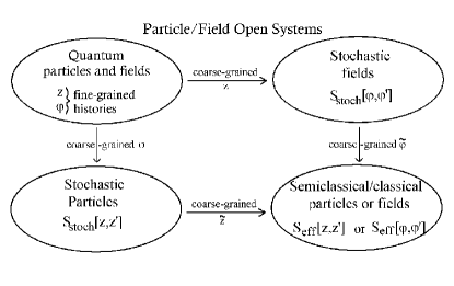
FIG. 1.: A schematic depiction of the relationship between the classical, semiclassical, stochastic, and quantum regimes.

FIG. 2.: Example of two oppositely charged particles in a background electric field, whose semiclassical motions $\bar{z}_{e^{\pm}}$ are in causally disjoint regions of spacetime. The radiation force $R_{12}$ vanishes, but the correlation-noise $N_{12}$ does not (for explanation see Sec. 5).

FIG. 3.: The closed-time-path manifold $M_{CTP}$ is composed of two copies of the ordinary spacetime manifold, $M_{1}$ and $M_{2},$ joined at a final-time hypersurface $\Sigma\left(t_{f}\right).$

REFERENCES

- [1] C. Cohen-Tannoudji, Atom-Photon Interactions (Wiley, New York, 1992); P. W. Milonni, Phys. Lett. 82A, 225 (1981).
- [2] W. G. Unruh, Phys. Rev. D 14, 870 (1976).
- [3] J. Schwinger, J. Math. Phys. 2, 407 (1961); L. Keldysh, Zh. Eksp. Teor. Fiz. 47, 1515 (1964), [Engl. tans. Sov. Phys. JEPT 20, 1018 (1965)].
- [4] E. Calzetta and B. L. Hu, Phys. Rev. D 35, 495 (1987).
- [5] E. Calzetta and B. L. Hu, Phys. Rev. D 37, 2878 (1988).
- [6] E. Calzetta and B. L. Hu, in Heat Kernel Techniques and Quantum Gravity, Vol. 4 of Discourses in Mathematics and Its Applications, Winnipeg, 1994, edited by S. Fulling (Texas AM University Press, College Station, TX, 1995), [Report No. hep-th/9501040].
- [7] E. Calzetta and B. L. Hu, Phys. Rev. D 025012 (2000).
- [8] G. N. Plass, Rev. Mod. Phys. 33, 37 (1961); F. Rohrlich, Am. J. Phys. 28, 639 (1969).
- [9] A. Raval, B. L. Hu, and J. R. Anglin, Phys. Rev. D 53, 7003 (1996).
- [10] B. L. Hu, Physica A158, 399 (1989).
- [11] R. P. Feynman and F. Vernon, Ann. Phys. 24, 118 (1963); R. P. Feynman and A. R. Hibbs, Quantum Mechanics and Path Integrals (McGraw-Hill, New York, 1965).
- [12] B. L. Hu, in Relativity and Gravitation: Classical and Quantum, Proceedings of the SILARG VII Symposium, Cocoyoc, Mexico, 1990, edited by J. D’Olivo (World Scientific, Singapore, 1991).
- [13] M. Gell-Mann and J. B. Hartle, Phys. Rev. D 47, 3345 (1993).
- [14] B. L. Hu, in Proc. Second International Workshop on Thermal Fields and their Applications, edited by H. Ezawa and et. al. (North-Holland, Amsterdam, 1991).
- [15] E. Joos and H. Zeh, Z. Phys. B 59, 2237 (1985); W. H. Zurek, Phys. Rev. D 24, 1516 (1981); M. Gell-Mann and J. B. Hartle, in Complexity, Entropy, and the Physics of Information, edited by W. H. Zurek (Addison-Wesley, Reading, 1990).
- [16] B. L. Hu, in Physical Origins of Time Asymmetry, edited by J. Perez-Mercader, J. J. Halliwell, and W. H. Zurek (Cambridge University Press, Cambridge, 1994), Chap. 34.
- [17] F. Dowker and A. Kent, Phys. Rev. Lett. 75, 3038 (1995).
- [18] M. Abraham and R. Becker, Electricity and Magnetism, Blackie, London, (1937); H. A. Lorentz, The Theory of Electrons (Dover Books, New York, 1952), pp. 49,253; P.A.M. Dirac, Proc. R. Soc. London A 167, 148 (1938).
- [19] J. B. Hartle, in Spacetime Quantum Mechanics and the Quantum Mechanics of Spacetime (1992), Les Houches lectures; H. F. Dowker and J. J. Halliwell, Phys. Rev. D 46, 1580 (1992); T. A. Brun, Phys. Rev. D 47, 3383 (1993).
- [20] A. O. Caldeira and A. J. Leggett, Ann. Phys. (N.Y.) 149, 374 (1983), and 153, 445(E) (1984); A. J. Leggett et al., Rev. Mod. Phys. 59, 1 (1987); A. O. Caldeira and A. J. Leggett, Physica A 121, 587 (1983); V. Hakim and V. Ambegaokar, Phys. Rev. A 32, 423 (1985); H. Grabert, P. Schramm, and G.-L. Ingold, Phys. Rev. Lett. 58, 1285 (1987).A. O. Caldeira and A. J. Leggett, Physica 121A, 587 (1988); B. L. Hu, J. P. Paz, and Y. Zhang, Phys. Rev. D 45, 2843 (1992).
- [21] B. L. Hu, J. P. Paz, and Y. Zhang, Phys. Rev. D 47, 1576 (1993).
- [22] F. Haake and R. Reibold, Phys. Rev. A 32, 2462 (1985); V. Hakim and V. Ambegaokar, Phys. Rev. A 32, 423 (1985).
- [23] P.R. Johnson and B. L. Hu, Stochastic Theory of Relativistic Particles Moving in a Quantum Field III. Electromagnetic Abraham-Lorentz-Dirac-Langevin Equation, Preprint (2000). A brief summary may be found in, P.R. Johnson and B. L. Hu, Worldline Influence Functional: Abraham-Lorentz-Dirac-Langevin Equation from QED, to appear in the proceedings of the second conference on Quantum Aspects of Beam Physics, edited by Pisin Chen, World Scientific, Singapore (2001), quant-ph/0012135.
- [24] E. Calzetta, S. Habib, and B. L. Hu, Phys. Rev. D 37, 2901 (1988); S. Habib and R. Laflamme, Phys. Rev. D 42, 4056 (1990).
- [25] W. H. Zurek, Phys. Rev. D 24, 1516 (1981); E. Joos and H. D. Zeh, Z. Phys. B 59, 223 (1985); W. G. Unruh and W. H. Zurek, Phys. Rev. D 40, 1071 (1989); A. O. Caldeira and A. J. Leggett, Phys. Rev. A 31, 1059 (1985).
- [26] G. W. Ford, J. T. Lewis, and R. F. O’Connell, Phys. Rev. Lett. 55, 2273 (1985); G. W. Ford, J. T. Lewis, and R. F. O’Connell, Phys. Rev. A 37, 4419 (1988).
- [27] G. W. Ford and R. F. O’Connell, Phys. Lett. A 157, 217 (1991).
- [28] G. W. Ford and R. F. O’Connell, Phys. Rev. A 57, 3112 (1998).
- [29] P. R. Johnson and B. L. Hu, Stochastic Theory of Relativistic Particles Moving in a Quantum Field: II. Scalar Abraham-Lorentz-Dirac-Langevin Equation, Radiation Reaction and Vacuum Fluctuations, quant-ph/0101001.
- [30] P. Barone and A. O. Caldeira, Phys. Rev. A 43, 57 (1991).
- [31] L. D. Romero and J. P. Paz, [preprint: quant-ph/9612036] (1996).
- [32] L. Diósi, Found. Phys. 20, 63 (1990).
- [33] L. H. Ford, Phys. Rev. D 47, 5571 (1993); L. H. Ford, Phys. Rev. A 56, 1812 (1997).
- [34] B. L. Hu and A. Matacz, Phys. Rev. D 49, 6612 (1994).
- [35] C. M. Smith and A. O. Caldeira, Phys. Rev. A 36, 3509 (1987); U. Weiss, Quantum Dissipative Systems, Vol. 2 of Series in Modern Condensed Matter Physics (World Scientific Publishing Co., Singapore, 1993); H. Kleinert, Path Integrals in Quantum Mechanics, Statistics and Polymer Physics (World Scientific, London, 1995).
- [36] P. R. Johnson and B. L. Hu, Worldline Influence Functional, Preprint (2000).
- [37] B. L. Hu and A. Matacz, Phys. Rev. D 51, 1577 (1995).
- [38] D. J. O’Conner, C. R. Stephens and B. L. Hu, Ann. Phys. (NY) 190, 310 (1987).
- [39] J. B. Hartle and S. H. Hawking, Phys. Rev. D 13, 2188 (1976).
- [40] I.H. Duru and N. Unal, Phys. Rev. D 34, 956 (1986).
- [41] R. Jordan, Phys. Rev. D 33, 444 (1986); B. S. DeWitt, in Quantum Concepts in Space and Time, edited by R. Penrose and C. Isham (Clarendon Press, Oxford, United Kingdom, 1986).
- [42] R. Kubo, Lectures in Theoretical Physics (Interscience, New York, 1959), Vol. 1, pp. 120–203; R. Kubo, Rep. Progr. Phys. (London) 29, 255 (1966).
- [43] P. R. Johnson, Ph.D. thesis, Appendix D, University of Maryland, College Park, 1999.
- [44] P. Bakshi and K. Mahanthappa, J. Math. Phys. 4, 1 (1963); K. Chou, Z. Su, B. Hao, and L. Yu, Phys. Rep 118, 1 (1985).
- [45] E. Calzetta and B. L. Hu, Phys. Rev. D 55, 3536 (1997); C. Kiefer, T. Padmanabhan, and T. Singh, Class. Quantum. Grav. 8, L185 (1991).
- [46] S. A. Ramsey, Ph.D. thesis, University of Maryland, College Park, 1997.
- [47] J. Schwinger, Phys. Rev. 82, 664 (1951); J. B. Hartle and S. H. Hawking, Phys. Rev. 13, 2188 (1976); C. Schubert, Acta. Phys. Pol. B 27, 3965, (1996).
- [48] B. L. Hu, G. Kang, and A. Matacz, Int. J. Mod. Phys A 9, 991 (1995).
- [49] R. Jackiw, Phys. Rev. D 9, 1686 (1974).
- [50] A. Raval, Ph.D. thesis, University of Maryland, College Park, 1996.