Continuously induced coherence without induced emission

Abstract

The coherence properties of two downconversion processes continuously coupled via idler beams are analyzed. We find that the amount of which-way information about a signal photon carried by idler beams periodically attains its maximum and minimum in the course of evolution. In correspondence with the famous experiments by Mandel’s group on the induced coherence without induced emission the coherence of signal beams is governed by that information. The ideal which-way measurement is constructed.

I Introduction

In famous experiments by Zou et al. and Wang et al. [1] it has been shown that the coherence of signal photons originating in two downconversion processes can be induced by making them indistinguishable. This has been accomplished by aligning the idler beam of the first process with the idler beam of the other, preventing the possibility to tell the signal photons originating in different crystals from each other based on the observation performed on the idler beams. Aligning the idler beams in this experiment in fact amounts to introducing a discrete (temporally localized) coupling of the two processes – the output of the first one being the input of the other. However, a discrete coupling is not the only possibility here. It is well known that many interesting dynamical and quantum-statistical phenomena arise as well from the continuous coupling of two or more optical processes [2]. A natural question arises whether also the interplay between quantum indistinguishability and coherence is reflected in the dynamics of two downconvertors experiencing continuous rather than discrete coupling. Such scheme would be a generalization of the original experimental setup of Zou et al. [1] which might exhibit richer phenomena. For example, one could imagine that the which-way information carried by the output idler beams of continuously coupled downconvertors could somehow depend on the length of the interaction region.

The analysis will be done in two steps. First, the coherence properties of two continuously coupled downconversion processes will be discussed for a particular choice of the relevant parameters. Then the setup will be replaced by two simpler devices – one resembling the experiment of Zou et al. [1] and the other being the two-photon interferometer of Ou et al. [3] – performing the same input-output transformations, which are more convenient for a general analysis in terms of which-way information.

II Induced coherence without induced emission

The setup of the thought experiment which will be discussed in the following is shown in Fig. 1. Two spontaneous downconvertors fed by strong coherent sources generate four downconverted modes, hereafter denoted $s_{1}$, $i_{1}$, $s_{2}$, $i_{2}$; $s$ and $i$ stands for “signal” and “idler”, respectively. Rather than cascading the downconvertors and aligning the idler beams as was proposed and realized by Zou et al. [1] we let the idler beams interact continuously. The conceptually simplest interaction between two modes is a linear energy exchange, which can be easily realized e.g. by means of evanescent waves [4]. At the output, the signal beams are superimposed at beamsplitter BS and then detected by detector $D$. The resulting interference pattern is scanned by varying the signal path difference.

The experimental setup in Fig. 1 (without beamsplitter BS) can be thought of as a single device described by the effective interaction momentum operator

$$\hat{G}=\hbar(\Gamma_{1}\hat{A}_{s_{1}}^{{\dagger}}\hat{A}_{i_{1}}^{{\dagger}}+\Gamma_{2}\hat{A}_{s_{2}}^{{\dagger}}\hat{A}_{i_{2}}^{{\dagger}}+\kappa\hat{A}_{i_{1}}\hat{A}_{i_{2}}^{{\dagger}}+{\rm h.c.}).$$ (1)

Here $\hat{A}_{k}$ is the annihilation operator of mode $k$, $\Gamma_{1}$ and $\Gamma_{2}$ are the effective strengths of the corresponding downconversion processes [5] and $\kappa$ is the strength of the linear interaction acting between modes $i_{1}$ and $i_{2}$. The unitary evolution operator generated by $\hat{G}$ reads $\hat{U}=\exp[i\hat{G}z/\hbar]$ and the spatial evolution of field operators is governed by the Heisenberg equations of motion

$$\frac{d\hat{A}_{s_{1}}}{dz}=i\Gamma_{1}\hat{A}_{i_{1}}^{{\dagger}}, \frac{d\hat{A}_{i_{1}}}{dz}=i\Gamma_{1}\hat{A}_{s_{1}}^{{\dagger}}+i\kappa^{\ast}\hat{A}_{i_{2}},$$ (2)

$$\frac{d\hat{A}_{s_{2}}}{dz}=i\Gamma_{2}\hat{A}_{i_{2}}^{{\dagger}}, \frac{d\hat{A}_{i_{2}}}{dz}=i\Gamma_{2}\hat{A}_{s_{2}}^{{\dagger}}+i\kappa^{\ast}\hat{A}_{i_{1}},$$ (3)

The device can operate in two very different regimes:

$$|\kappa|<|\Gamma_{1}|+|\Gamma_{2}| \mbox{above threshold},$$ (4)

$$|\kappa|>|\Gamma_{1}|+|\Gamma_{2}| \mbox{below threshold}.$$ (5)

Above the threshold the intensity of downconverted light grows exponentially with increasing interaction length $L$, whereas below the threshold all modes exhibit oscillations. We will mainly be interested in the coherence of the signal beams. We define the (normalized) mutual coherence of signal beams $\gamma$ through the relation

$$i\gamma\equiv\frac{\langle\hat{A}^{{\dagger}}_{s_{1}}\hat{A}_{s_{2}}\rangle}{\sqrt{\langle\hat{A}^{{\dagger}}_{s_{1}}\hat{A}_{s_{1}}\rangle\langle\hat{A}^{{\dagger}}_{s_{2}}\hat{A}_{s_{2}}\rangle}},$$ (6)

where the imaginary unit $i$ has been factored out in order to make $\gamma$ a real quantity. In principle there are two ways how the signal beams originating in two spontaneous downconvertors can become coherent. Either the coherence can be induced by the emission of signal photons stimulated by idler photons traversing from one medium to the other one, or, as was shown in [1], it can originate in the principal indistinguishability of signal photons. In experiments of Zou et al. the former (classical) cause of coherence was eliminated simply by keeping the low rate of generation of downconverted photon pairs. This can be easily imitated with our setup in Fig. 1. We have already mentioned that below threshold the intensities of all the four downconverted modes oscillate. It can be shown that the amplitude of the oscillations decreases with increasing strength $\kappa$ of the linear interaction [6]. This is caused by the effective phase mismatch introduced by the continuos interaction (see also the discussion in section IV). We note that such an inhibition of downconversion process by coupling it to another mode or process can alternatively be interpreted as the quantum Zeno effect [7, 8], the linear coupling being a sort of continuous measurement [9, 6]. Hence for sufficiently strong coupling strength $\kappa$, the intensities of all the involved modes keep low, and spontaneous emission dominates in the course of evolution.

A typical behavior of the mutual coherence function (6) well below threshold is shown in Fig. 2 (solid line). A characteristic resonant feature can be seen in Fig. 2 repeating regularly. The coherence of the signal modes periodically attains its maximum allowed values $\pm 1$ and hence the signal modes become fully coherent every now and then. We remind the reader that this coherence is not induced by a stimulated emission because the rate of the emissions stimulated by the exchanged idler photons remains very small compared to the rate of spontaneous emissions. This is due to the small mean number of photons present in the system (see Fig. 2, dotted line). Analogously to Zou et al. [1] we claim that for the corresponding interaction lengths the state of the output light is such that no matter what measurement is performed on the output idler modes, no information about the mode in which the signal photon has left the coupled downconvertors is gained; the probability of having more than one output signal photon being very small. Similarly it is tempting to state that roots of $\gamma$ imply the presence of a perfect which-way information about the signal photon in the idler modes for these interaction lengths. This would correspond to preventing the first idler beam from reaching the second crystal in the experiment by Zou et al. [1].

III Substituting schemes

A Modified setup of Zou et al.

Although it is possible to obtain analytical solutions of the system (2), they are awkward and not suitable for physical discussion. We will adopt a different strategy. With the assumption that the strengths $\Gamma_{1},\Gamma_{2}$ and $\kappa$ are real (without loss of generality), the momentum operator (1) can be written as a linear combination

$$\hat{G^{\prime}}=\hbar(\Gamma_{1}\hat{X}_{1}+\Gamma_{2}\hat{X}_{2}+\kappa\hat{X}_{3}),$$ (7)

of Hermitian generators

$$\hat{X}_{1} = \hat{A}_{s_{1}}\hat{A}_{i_{1}}+\hat{A}_{s_{1}}^{{\dagger}}\hat{A}_{i_{1}}^{{\dagger}},\quad\hat{X}_{2}=\hat{A}_{s_{2}}\hat{A}_{i_{2}}+\hat{A}_{s_{2}}^{{\dagger}}\hat{A}_{i_{2}}^{{\dagger}}$$ (9)

$$\hat{X}_{3}=\hat{A}_{i_{1}}\hat{A}_{i_{2}}^{{\dagger}}+\hat{A}_{i_{1}}^{{\dagger}}\hat{A}_{i_{2}}.$$

These, together with other three Hermitian generators,

$$\hat{X}_{4} = i(\hat{A}_{s_{1}}\hat{A}_{i_{2}}-\hat{A}_{s_{1}}^{{\dagger}}\hat{A}_{i_{2}}^{{\dagger}}),\enspace\hat{X}_{5}=i(\hat{A}_{i_{1}}\hat{A}_{s_{2}}-\hat{A}_{i_{1}}^{{\dagger}}\hat{A}_{s_{2}}^{{\dagger}})$$ (11)

$$\hat{X}_{6}=\hat{A}_{s_{1}}\hat{A}_{s_{2}}^{{\dagger}}+\hat{A}_{s_{1}}^{{\dagger}}\hat{A}_{s_{2}},$$

comprise a closed six dimensional algebra

$$[\hat{X}_{i},\hat{X}_{j}]=iC_{ij}^{k}\hat{X}_{k},\quad i,j,k=1,..,6.$$ (12)

The real structure coefficients $C_{ij}^{k}$ need not be specified here; note only that $[\hat{X}_{1},\hat{X}_{2}]=[\hat{X}_{3},\hat{X}_{6}]=[\hat{X}_{4},\hat{X}_{5}]=0$. Closeness of the algebra (12) guarantees the possibility to decompose the evolution operator of the system as follows

$$e^{\frac{i}{\hbar}\hat{G}z} = e^{ig_{5}(z)\hat{X}_{5}}e^{ig_{4}(z)\hat{X}_{4}}e^{ig_{1}(z)\hat{X}_{1}}e^{ig_{2}(z)\hat{X}_{2}}$$ (14)

$$\times e^{ig_{3}(z)\hat{X}_{3}}e^{ig_{6}(z)\hat{X}_{6}}.$$

Physically, this corresponds to replacing the discussed experimental setup with a sequence of simpler devices like downconvertors ($\hat{X}_{1}$, $\hat{X}_{2}$, $\hat{X}_{4}$, $\hat{X}_{5}$), and beamsplitters ($\hat{X}_{3}$, $\hat{X}_{6}$) generating the same output fields [10]. To a given interaction length $L$ of the original device (1) there corresponds a substituting scheme (14) with a particular choice of the coupling parameters, $g_{i}=g_{i}(L)$. The reasons for substituting the original device are twofold. First, for the given values of the parameters $g_{i}$ the input-output transformation provided by the substituting scheme is relatively simple, thus suitable for physical discussion. Moreover, well below threshold, where all the output intensities are low, the parameters $g_{1}$, $g_{2}$, $g_{4}$, and $g_{5}$ of the downconvertors of the corresponding substituting scheme are expected to be small. Then one can solve for the input-output transformation to only a low order in those four parameters resulting in further simplifications. In this way the long-time dynamics of the original device (Fig. 1) is mapped into the short-time dynamics of the substituting scheme.

Since we are only interested in the spontaneous process where all the modes of the original device start from vacuum the presence of beamsplitters $\hat{X}_{3}$ and $\hat{X}_{6}$ in the substituting scheme is irrelevant [their exponential operators act on vacuum]. This is why the particular ordering in (14) has been chosen. The remaining four downconvertors, see Fig. 3, constitute the sought substituting scheme which, for input vacuum states, is equivalent to the original setup (Fig. 1). Here the links between the experiment on the induced emission [1] and our continuously coupled device start to appear. Two simultaneous experimental arrangements of Zou et al. can be recognized in Fig. 3; one being formed by downconvertors $1$ and $5$, the other being formed by the remaining two. This similarity will help us to explain the induced coherence observed in Fig. 2.

In order to keep algebra simple we will assume that at most one downconverted pair of photons is present in the substituting scheme. This is usually a good approximation under standard experimental conditions. This also corresponds to the situation when the original device operates well below threshold, see Fig. 2. Low mean number of output signal photons implies small magnitudes of nonlinearities $|g_{i}|$, as can be seen from the following inequality,

$$\langle\hat{n}_{s_{1}}\rangle+\langle\hat{n}_{s_{2}}\rangle \geq \sinh^{2}g_{1}+\sinh^{2}g_{2}+\sinh^{2}g_{4}$$ (16)

$$+\sinh^{2}g_{5},$$

which immediately yields an upper bound on $|g_{i}|$,

$$|g_{i}|\leq\sinh^{-1}(\sqrt{\langle\hat{n}_{s_{1}}\rangle+\langle\hat{n}_{s_{2}}\rangle}).$$ (17)

The evolution operator of the first pair of downconvertors in Fig. 3 to the first order in the nonlinear coupling parameters reads

$$U_{1}=1+ig_{1}\hat{A}^{{\dagger}}_{s_{1}}\hat{A}^{{\dagger}}_{i_{1}}+ig_{2}\hat{A}^{{\dagger}}_{s_{2}}\hat{A}^{{\dagger}}_{i_{2}}.$$ (18)

Similarly, the evolution of the second pair of downconvertors is governed by the operator

$$U_{2}=1+g_{4}\hat{A}^{{\dagger}}_{s_{1}}\hat{A}^{{\dagger}}_{i_{2}}+g_{5}\hat{A}^{{\dagger}}_{s_{2}}\hat{A}^{{\dagger}}_{i_{1}}.$$ (19)

Note that annihilation operators do not contribute to Eqs. (18) and (19) because we assume that at most one pair of photons is created in the substituting scheme.

The input vacuum state develops into the output state

$$|\Psi\rangle \approx (1-|{\rm vac}\rangle\langle{\rm vac}|)U_{2}U_{1}|{\rm vac}\rangle\approx g_{4}|1001\rangle+g_{5}|0110\rangle$$ (21)

$$+ig_{1}|1100\rangle+ig_{2}|0011\rangle,$$

where the redundant vacuum component has been projected out and only terms to the first order in the nonlinear coupling parameters have been kept. We have introduced a short-hand notation $|n_{1}n_{2}n_{3}n_{4}\rangle\equiv|n_{1}\rangle_{s_{1}}|n_{2}\rangle_{i_{1}}|n_{3}\rangle_{s_{2}}|n_{4}\rangle_{i_{2}}$. Here and in the following we omit unimportant normalization factors. The mutual coherence of the signal beams is, according to Eq. (6), given by the transition probability amplitude between the states

$$\hat{A}_{s_{2}}|\Psi\rangle = g_{5}|0100\rangle+ig_{2}|0001\rangle,$$ (22)

$$\hat{A}_{s_{1}}|\Psi\rangle = ig_{1}|0100\rangle+g_{4}|0001\rangle.$$ (23)

It is convenient to define two vectors whose components are proportional to the nonlinear coupling parameters of the four downconvertors,

$${\bf u}=\left(\begin{array}[]{c}g_{1}\\ g_{4}\\ 0\end{array}\right),\qquad{\bf v}=\left(\begin{array}[]{c}g_{5}\\ -g_{2}\\ 0\end{array}\right).$$ (24)

In terms of vectors ${\bf u}$ and ${\bf v}$, the normalized mutual coherence of signal beams reads

$$|\gamma|^{2}=\frac{|{\bf u}\cdot{\bf v}|^{2}}{u^{2}v^{2}}=\frac{(g_{1}g_{5}-g_{2}g_{4})^{2}}{(g_{1}^{2}+g_{4}^{2})(g_{2}^{2}+g_{5}^{2})}.$$ (25)

The calculation of the mutual coherence of signal beams thus has been reduced to considering the mutual geometry of the vectors ${\bf u}$ and ${\bf v}$. If the parameters of the substituting scheme are such that the vectors are orthogonal, the mutual coherence $\gamma$ vanishes and the signal beams do not interfere. In the opposite extreme case when the vectors ${\bf u}$ and ${\bf v}$ are almost collinear, the mutual coherence attains its maximum magnitude and the signal beams become first-order coherent. An example of the latter situation is the experiment of Zou et al. [1], which is a special case of the setup in Fig. 3 with $g_{1}=g_{5}=0$ or $g_{2}=g_{4}=0$.

In the following we will show that the mutual coherence of signal beams strongly depends on the amount of the which-way information about them that is carried by the idler beams. Before any measurement on the system is attempted, the only which-way information about the signal photon that is available arises from different intensities of signal beams. This information will be called prior which-way information. Provided the idler beams carry information about the signal photon, the prior which-way information can be updated by performing a suitable measurement on them.

First let us discuss the incoherent case. When the vectors ${\bf u}$ and ${\bf v}$ are orthogonal, the output state $|\Psi\rangle$ can be rewritten as follows,

$$|\Psi\rangle=\frac{g_{2}}{g_{1}}|\varphi_{1}\rangle_{i}|01\rangle_{s}+|\varphi_{2}\rangle_{i}|10\rangle_{s},\quad({\bf u}\perp{\bf v})$$ (26)

where the states $|\varphi_{1}\rangle$ and $|\varphi_{2}\rangle$ of the idler beams,

$$|\varphi_{1}\rangle = g_{4}|10\rangle_{i}+ig_{1}|01\rangle_{i},$$ (27)

$$|\varphi_{2}\rangle = ig_{1}|10\rangle_{i}+g_{4}|01\rangle_{i},$$ (28)

are orthogonal. This means that there is a measurement on the idler beams yielding a perfect which-way information about the signal photon, for instance, the measurement having the spectral decomposition

$$\hat{S}=|\varphi_{1}\rangle\langle\varphi_{1}|-|\varphi_{2}\rangle\langle\varphi_{2}|.$$ (29)

If the outcome corresponding to $|\varphi_{1}\rangle$ is detected the signal photon is projected to mode $s_{2}$. If, on the other hand, $|\varphi_{2}\rangle$ is detected, the signal photon is projected to mode $s_{1}$. Perfect knowledge of the signal photon’s path precludes the interference. Provided the parameters of the substituting scheme are such that the vectors ${\bf u}$ and ${\bf v}$ are not completely orthogonal, the decomposition (26) with orthogonal states of the idler beams is not possible; the knowledge of the signal photon’s path is then only partial. Nevertheless, one can still think of the measuring apparatus (29) as of the ideal which-way apparatus – ideal in the sense that it gives perfect which-way knowledge in the limit ${\bf u}\cdot{\bf v}\rightarrow 0$. Eigenvectors of $\hat{S}$ can be used to decompose the output state $|\Psi\rangle$ in the spirit of (26),

$$|\Psi\rangle = |{\bf u}\times{\bf v}|\,|\varphi_{1}\rangle_{i}|01\rangle_{s}$$ (30)

$$+ |\varphi_{2}\rangle_{i}(-i{\bf u}\cdot{\bf v}|01\rangle_{s}+{\bf u}^{2}|10\rangle_{s}).$$ (31)

Now, the gained amount of information about the signal photon will depend on the outcome of the measurement of $\hat{S}$. If the result $|\varphi_{1}\rangle$ is detected, the signal photon will be localized in the mode $s_{2}$ with certainty, and therefore it will not contribute to the interference pattern. If, however, we end up with the result $|\varphi_{2}\rangle$, the state of the signal photon will become a coherent superposition of states “photon being in mode $s_{1}$” and “photon being in mode $s_{2}$”, and $|\gamma|$ attains the maximum value of one. Since both the outcomes occur in random, the mutual coherence $|\gamma|$ becomes a weighted sum of zero and one. As the angle between the vectors ${\bf u}$ and ${\bf v}$ gets smaller, the probability of the former unambiguous case to happen gets smaller, too. When the vectors become collinear, the output state (21) becomes a factorized state. In this case, the state of the signal field after the measurement will be the pure superposition

$$|\Psi\rangle_{s}=\pm iv|01\rangle_{s}+u|10\rangle_{s},\qquad({\bf u}\,\|\,{\bf v}),$$ (32)

and the mutual coherence will be maximum, in agreement with Eq. (25). Because the diagonal elements of the state (32) in $\{|10\rangle_{s},|01\rangle_{s}\}$ basis are the same as those of the pre-measurement state (21), the posterior which-way information equals the prior which-way information and no additional which-way information is gained by the measurement.

It is interesting to look closely at the measurement $\hat{S}$ and its relation to the optimum which-way measurement in the experiment of Zou et al. which is nothing else than the counting of idler photons in modes $i_{1}$ and $i_{2}$. Eigenvectors of $\hat{S}$ (27) can be parameterized by an angle $\phi$,

$$|\varphi_{1}\rangle=\sin\phi|10\rangle_{i}+i\cos\phi|01\rangle_{i},$$ (33)

$$|\varphi_{2}\rangle=i\cos\phi|10\rangle_{i}+\sin\phi|01\rangle_{i},$$ (34)

$$\sin\phi=\frac{g_{4}}{\sqrt{g_{1}^{2}+g_{4}^{2}}}.$$ (35)

Hence the measurement $\hat{S}$ can be rewritten in terms of the $z$-component of the Stokes operator acting on the two-mode idler field, $\hat{S}_{z}=|01\rangle\langle 01|-|10\rangle\langle 10|$,

$$\hat{S}=e^{-i\hat{\sigma}_{y}\phi}\hat{S}_{z}e^{i\hat{\sigma}_{y}\phi},$$ (36)

where $\hat{\sigma}_{y}$ is Pauli matrix. Notice that on the subspace of the Hilbert space of the idler modes with the total number of idler photons $n_{i_{1}}+n_{i_{2}}=1$ the operator $\hat{S}_{z}$ is just the measurement of the difference of the numbers of photons in modes $i_{2}$ and $i_{1}$, $\hat{S}_{z}=\hat{n}_{i_{2}}-\hat{n}_{i_{1}}$. This is the ideal which-way measurement in the experiments of Zou et al. Here the situation is similar. The ideal which-way detection differs from it only by a rotation given by the coupling parameters of the substituting scheme.

The parameters of the substituting scheme can be found by differentiating both sides of Eq. (14) and rearranging the right-hand side [11]. In this way one obtains a system of nonlinear differential equations for the sought parameters, which can be solved by numerical integration. There is also another approach [10] which makes use of correlation functions and the fact that all the input modes are in the vacuum state. This procedure yields explicit expressions for the unknown parameters $g_{i}$, see Appendix.

The oriented angle between the vectors ${\bf u}$ and ${\bf v}$ characterizing the substituting scheme is displayed in Fig. 4 for the same coupling strengths of the original device as that in Fig. 2. Notice that zeros/maxima of the signal mutual coherence in Fig. 2 indeed coincide with the interaction lengths for which the vectors ${\bf u}$ and ${\bf v}$ become orthogonal/parallel, in agreement with Eq. (25). One can also check that all the coupling parameters of the active elements are small; in this case it holds that $|g_{1,2,4,5}|\leq 0.2$. Since the probability of having more than one photon pair in the substituting scheme scales as $\sum_{i}g_{i}^{4}$, the approximations (18) and (19) are fully justified well below threshold. This proves our claim that also in the case of continuously coupled downconvertors the coherence of signal beams is governed by the principal indistinguishability of signal photons. Our device can thus be regarded as an interesting generalization of the experimental setup of Zou et al. where the distinguishability of signal photons can be controlled by the length of the device itself rather than by using auxiliary optical elements.

B Setup of Ou et al.

An alternative representation of two continuously coupled downconvertors is possible. It has been shown in [12] that any four-mode unitary transformation leaving the set of Gaussian states invariant can be realized by using only four single-mode squeezers placed in between two four-port linear interferometers. In our case we can further simplify such scheme if we use two-mode squeezers (nondegenerate downconvertors) instead of single-mode squeezers. The continuously coupled downconvertors can be replaced with a sequence of two beamsplitters followed by two downconvertors and another two beamsplitters. Since we consider spontaneous process, the first pair of beamsplitters can be omitted, see Fig. 5. Notice that actually this is the same arrangement as the well-known two-photon interferometer of Ou et al. [3]. Its four relevant parameters, the nonlinear coupling parameters $g_{1}$ and $g_{2}$ of the two downconvertors, and the mixing angles $\phi_{s}$, $\phi_{i}$ of the two beamsplitters are determined by the coupling strengths $\Gamma_{1}$, $\Gamma_{2}$, $\kappa$, and the interaction length $L$ of the original continuously coupled device.

The mutual coherence of signal beams can now be expressed as

$$\gamma=\frac{\langle\hat{n}_{s_{1}}\rangle-\langle\hat{n}_{s_{2}}\rangle}{\sqrt{4\langle\hat{N}_{s_{1}}\rangle\langle\hat{N}_{s_{2}}\rangle}}\sin(2\phi_{s}),$$ (37)

where

$$\langle\hat{N}_{s_{1}}\rangle = \langle\hat{n}_{s_{1}}\rangle\cos^{2}\phi_{s}+\langle\hat{n}_{s_{2}}\rangle\sin^{2}\phi_{s},$$ (38)

$$\langle\hat{N}_{s_{2}}\rangle = \langle\hat{n}_{s_{1}}\rangle\sin^{2}\phi_{s}+\langle\hat{n}_{s_{2}}\rangle\cos^{2}\phi_{s},$$ (39)

and

$$\langle\hat{n}_{s_{j}}\rangle=\sinh^{2}g_{j}$$ (40)

are mean numbers of photons in signal modes at the output of the two downconvertors. The degree of coherence $\gamma$ depends on the mixing angle $\phi_{s}$ of the signal beamsplitter. However, more important is the dependence on the difference of the mean numbers of photons $\langle\hat{n}_{s_{j}}\rangle$. If $g_{1}=g_{2}$, then $\langle\hat{n}_{s_{1}}\rangle=\langle\hat{n}_{s_{2}}\rangle$ and $\gamma=0$. On the other hand, if $g_{1}=0$ or $g_{2}=0$ then $|\gamma|=1$ irrespective of $\phi_{s}$ and the two output signal modes are fully coherent. If the two continuously coupled downconvertors effectively behave like a single downconvertor followed by beamsplitters, then the two output signal modes stem from a single mode in chaotic state mixed with vacuum at a beamsplitter. This leads to the full coherence of the two output signal modes. On the other hand, if the device effectively behaves like two identical downconvertors then both signal modes mixed at BS_s are in chaotic state with the same mean numbers of photons $\langle\hat{n}_{s_{1}}\rangle=\langle\hat{n}_{s_{2}}\rangle$ and no coherence can be observed at the output. When the interaction length $L$ is varied one can continuously move from the regime where one downconvertor is dominant to the regime where both downconvertors have comparable output. These transitions result in sharp peaks observed in Fig. 2. A typical behavior of parameters $g_{1}$ and $g_{2}$ is shown in Fig. 6. Notice that interaction lengths for which one of the parameters is zero or $|g_{1}|=|g_{2}|$ correspond to full or no coherence in Fig. 2.

The analysis of the coherence properties of continuously coupled downconvertors in terms of which-way information presented in the previous subsection can equivalently be done using the present scheme. Since the analysis would lead to the same interpretation as in previous subsection we do not repeat it here. We just note that it follows from Eq. (40) that the parameters $g_{1}$ and $g_{2}$ of the present substituting scheme are small well below the threshold where the output intensity is low, see also Fig. 6.

Having seen that one device – two continuously coupled downconvertors – can be replaced with two different schemes resembling two famous experiments one may ask whether the experimental arrangements themselves are in some sense equivalent. The affirmative answer of course stems from the fact that both the experiments [1] and [3] utilize the same optical elements whose action falls to the same group of transformations. Just for completeness let us show how the two-photon interferometer (Fig. 5) can be used to analyze the experiment on the induced coherence without induced emission [1]. The setup consists of two downconvertors with parameters $r_{1}$ and $r_{2}$. The idler mode coming from the first crystal is partially injected in the second one. This is realized, e.g. by placing a beamsplitter with mixing angle $\psi$ in between them. The input-output transformation of this device reads [13]

$$\hat{A}_{s_{1},\rm out} = \hat{A}_{s_{1}}\cosh r_{1}+i\hat{A}_{i_{1}}^{\dagger}\sinh r_{1},$$ (41)

$$\hat{A}_{s_{2},\rm out} = -i\hat{A}_{s_{1}}\sinh r_{1}\sin\psi\sinh r_{2}+\hat{A}_{s_{2}}\cosh r_{2}$$ (43)

$$+\hat{A}_{i_{1}}^{\dagger}\cosh r_{1}\sin\psi\sinh r_{2}+i\hat{A}_{i_{2}}^{\dagger}\cos\psi\sinh r_{2},$$

$$\hat{A}_{i_{1},\rm out} = i\hat{A}_{s_{1}}^{\dagger}\sinh r_{1}\cos\psi$$ (45)

$$+\hat{A}_{i_{1}}\cosh r_{1}\cos\psi+i\hat{A}_{i_{2}}\sin\psi,$$

$$\hat{A}_{i_{2},\rm out} = -\hat{A}_{s_{1}}^{\dagger}\sinh r_{1}\sin\psi\cosh r_{2}+i\hat{A}_{s_{2}}^{\dagger}\sinh r_{2}$$ (47)

$$+i\hat{A}_{i_{1}}\cosh r_{1}\sin\psi\cosh r_{2}+\hat{A}_{i_{2}}\cos\psi\cosh r_{2}.$$

In the original setup of Zou et al. the mutual coherence of the signal beams was controlled by the value of mixing angle $\psi$. When the idler beams were perfectly superposed, $\psi=\pi/2$, the signal beams were fully coherent, $|\gamma|=1$, because the idler photons did not contain any which-way information. In the opposite extreme $\psi=0$, the signal modes were completely incoherent, $\gamma=0$, because the idler photons in principle could allow one to determine whether the signal photon had come from the first or the second downconvertor.

Let us now show how this dependence of $\gamma$ on $\psi$ is reflected in the substituting scheme shown in Fig. 5. In Fig. 7 we plot $\gamma$ and $g_{1}$, $g_{2}$ as functions of the mixing angle $\psi$. As could be expected, $\gamma$ increases with $\psi$ from $0$ at $\psi=0$ to $1$ at $\psi=\pi/2$. Also the squeezing constant $g_{1}$ increases with $\psi$, while $g_{2}$ decreases and reaches $0$ at $\psi=\pi/2$. The coherence $\gamma$ increases with growing ratio $g_{1}/g_{2}$ in agreement with Eq. (37). If the idler modes of the two downconvertors are perfectly aligned, then the whole setup is equivalent to a single downconvertor followed by a beamsplitter. Since there is only one source of signal photons in this case, the output signal beams are fully coherent.

IV Discussion and conclusions

We have found that idler beams of two continuously coupled downconvertors become periodically strongly correlated (uncorrelated) with signals in the course of evolution. This is reflected in the entangled (disentangled) nature of the signal-idler field (26) and resembles the interaction of a quantum system (signal modes) with a quantum meter (idler modes). One may loosly say that the signal modes are periodically “observed” by the idler modes. Yet one has to realize that no bona fide measurement is being performed in this way. An essential part of any such measurement – the reading of the quantum meter by a classical apparatus – is missing here. The signal field is not projected but continues the unitary evolution. Nevertheless, the entanglement of signal and idler fields, which is responsible for destroying the signal coherence is enough to disturb the phase relations between interacting modes and slow down the downconversion process [8]. As the coupling of idler modes becomes stronger the frequency of “observations” of the signal field by the idler one increases. In the limit of very large $\kappa$ the two downconversion processes become completely frozen and no photon pairs are being created anymore. This effect, usually called the quantum Zeno effect [7], provides an alternative explanation of why two strongly coupled downcorvertors operate below threshold. Similar situation in another experimental setup has been analyzed in [6]. This effect has been interpreted as the quantum Zeno effect caused by a continuous observation of one mode of light by another one. It is well known that frequently repeated measurements and continuous observation (or interactions) can hinder evolution of a quantum system in a similar way [14]. Some quantitative statements relating the frequency of discrete measurements to the strength of continuous interactions having the same effect can even be found in the literature [15]. The experimental arrangement discussed in this paper is an interesting example of a system where such discrete disturbances naturally arise from a continuous interaction between its constituent parts.

Parameters of the substituting schemes

This derivation closely follows the general procedure of Ref. [10], Sec. IIC. In the Heisenberg picture, the vector of operators

$${\bf\hat{A}}=\left(\begin{array}[]{c}\hat{A}_{s_{1}}\\ \hat{A}_{s_{2}}\\ \hat{A}_{i_{1}}^{\dagger}\\ \hat{A}_{i_{2}}^{\dagger}\end{array}\right)$$ (49)

transforms according to

$${\bf\hat{A}}_{\rm out}={\bf M}{\bf\hat{A}}_{\rm in},$$ (50)

where ${\bf M}=\exp(i{\bf H}L)$ and

$${\bf H}=\left(\begin{array}[]{cccc}0&0&\Gamma_{1}&0\\ 0&0&0&\Gamma_{2}\\ -\Gamma_{1}&0&0&-\kappa\\ 0&-\Gamma_{2}&-\kappa&0\end{array}\right).$$ (51)

In order to find analytical expressions for the parameters of the substituting schemes, we consider output state generated from the vacuum and propagate this state backward through the schemes. At each step, some correlations between the four modes vanish, which provides us with equations for the unknown parameters. Let us begin with the scheme shown in Fig. 3. When we propagate the output modes in front of the second pair of downconvertors, we get

$\displaystyle{\bf\hat{A}}_{\rm c}={\bf M}_{45}{\bf\hat{A}}_{\rm out},$

where

$${\bf M}_{45}=\left(\begin{array}[]{cccc}\cosh g_{4}&0&0&-\sinh g_{4}\\ 0&\cosh g_{5}&-\sinh g_{5}&0\\ 0&-\sinh g_{5}&\cosh g_{5}&0\\ -\sinh g_{4}&0&0&\cosh g_{4}\end{array}\right).$$ (52)

The modes $s_{1,c}$ and $i_{1,c}$ are not correlated with $s_{2,c}$ and $i_{2,c}$. In particular,

$$\langle\Delta\hat{A}_{s_{1},\rm c}\Delta\hat{A}_{i_{2},\rm c}\rangle=0,\qquad\langle\Delta\hat{A}_{s_{2},\rm c}\Delta\hat{A}_{i_{1},\rm c}\rangle=0.$$ (53)

We can solve these two equations for the parameters $g_{4}$ and $g_{5}$,

$$\tanh(2g_{4})=\frac{2D_{s_{1}i_{2},\rm out}}{B_{s_{1},\rm out}+B_{i_{2},\rm out}+1},$$ (54)

$$\tanh(2g_{5})=\frac{2D_{s_{2}i_{1},\rm out}}{B_{s_{2},\rm out}+B_{i_{1},\rm out}+1}.$$ (55)

where

$$D_{jk,\rm out} = \langle\Delta\hat{A}_{j,\rm out}\Delta\hat{A}_{k,\rm out}\rangle,$$ (56)

$$B_{j,\rm out} = \langle\Delta\hat{A}_{j,\rm out}^{\dagger}\Delta\hat{A}_{j,\rm out}\rangle.$$ (57)

Since all the input modes are in vacuum state it is easy to express the correlations (57) in terms of the elements of matrix $\bf M$ [10]. We find,

$$D_{s_{1}i_{1},\rm out} = M_{11}M_{31}^{\ast}+M_{12}M_{32}^{\ast},$$ (58)

$$D_{s_{1}i_{2},\rm out} = M_{11}M_{41}^{\ast}+M_{12}M_{42}^{\ast},$$ (59)

$$D_{s_{2}i_{1},\rm out} = M_{21}M_{31}^{\ast}+M_{22}M_{32}^{\ast},$$ (60)

$$D_{s_{2}i_{2},\rm out} = M_{21}M_{41}^{\ast}+M_{22}M_{42}^{\ast},$$ (61)

$$B_{s_{1},\rm out} = |M_{13}|^{2}+|M_{14}|^{2},$$ (62)

$$B_{s_{2},\rm out} = |M_{23}|^{2}+|M_{24}|^{2},$$ (63)

$$B_{i_{1},\rm out} = |M_{31}|^{2}+|M_{32}|^{2},$$ (64)

$$B_{i_{2},\rm out} = |M_{41}|^{2}+|M_{42}|^{2}.$$ (65)

In the next step we propagate ${\bf\hat{A}}_{\rm c}$ back in front of the first pair of downconvertors, ${\bf\hat{A}}_{\rm in}={\bf M}_{12}{\bf\hat{A}}_{\rm c}$,

$${\bf M}_{12}=\left(\begin{array}[]{cccc}\cosh g_{1}&0&-i\sinh g_{1}&0\\ 0&\cosh g_{2}&0&-i\sinh g_{2}\\ i\sinh g_{1}&0&\cosh g_{1}&0\\ 0&i\sinh g_{2}&0&\cosh g_{2}\end{array}\right).$$ (66)

Since the input modes are in vacuum states, all correlations should vanish. In particular, we have

$$\langle\Delta\hat{A}_{s_{1},\rm in}\Delta\hat{A}_{i_{1},\rm in}\rangle=0,\qquad\langle\Delta\hat{A}_{s_{2},\rm in}\Delta\hat{A}_{i_{2},\rm in}\rangle=0.$$ (67)

Upon solving the Eqs. (67) for the parameters $g_{1}$ and $g_{2}$, we get

$$\tanh(2g_{1})=\frac{-2iD_{s_{1}i_{1},\rm c}}{B_{s_{1},\rm c}+B_{i_{1},\rm c}+1},$$ (68)

$$\tanh(2g_{2})=\frac{-2iD_{s_{2}i_{2},\rm c}}{B_{s_{2},\rm c}+B_{i_{2},\rm c}+1}.$$ (69)

The correlations $D_{jk,\rm c}$ and $B_{j,\rm c}$ of operators $\hat{A}_{j,\rm c}$ can be expressed in terms of the elements of the matrix ${\bf M}_{\rm c}={\bf M}_{45}{\bf M}$. One can directly use Eq. (65) where $\bf M$ is replaced with ${\bf M}_{\rm c}$. We note that $D_{s_{1}i_{1},\rm c}$ and $D_{s_{2}i_{2},\rm c}$ are purely imaginary hence the right-hand sides of Eq. (69) are real.

The calculation of the parameters of the substituting scheme shown in Fig. 5 proceeds along similar lines. We propagate the output modes in front of the beamsplitters, ${\bf\hat{A}}_{\rm c}={\bf M}_{\phi}{\bf M}{\bf\hat{A}}_{\rm in}$, where

$${\bf M}_{\phi}=\left(\begin{array}[]{cccc}\cos\phi_{s}&-i\sin\phi_{s}&0&0\\ -i\sin\phi_{s}&\cos\phi_{s}&0&0\\ 0&0&\cos\phi_{i}&i\sin\phi_{i}\\ 0&0&i\sin\phi_{i}&\cos\phi_{i}\end{array}\right).$$ (70)

The conditions (53) provide system of two coupled equations for $\tan\phi_{s}$ and $\tan\phi_{i}$ whose solution reads

$$\tan\phi_{s} = \frac{D_{s_{1}i_{2},\rm out}-iD_{s_{1}i_{1},\rm out}\tan\phi_{i}}{D_{s_{2}i_{1},\rm out}\tan\phi_{i}+iD_{s_{2}i_{2},\rm out}},$$ (71)

$$\tan\phi_{i} = \frac{1}{2}(-p\pm\sqrt{p^{2}+4}),$$ (72)

where

$$p=i\frac{D_{s_{1}i_{1},\rm out}^{2}+D_{s_{1}i_{2},\rm out}^{2}-D_{s_{2}i_{1},\rm out}^{2}-D_{s_{2}i_{2},\rm out}^{2}}{D_{s_{1}i_{1},\rm out}D_{s_{1}i_{2},\rm out}-D_{s_{2}i_{1},\rm out}D_{s_{2}i_{2},\rm out}}.$$ (73)

When we know $\phi_{s,i}$ we calculate the matrix ${\bf M}_{\rm c}={\bf M}_{\phi}{\bf M}$ and determine the parameters $g_{1}$ and $g_{2}$ from Eq. (69).

The above formulas also enable us to find the parameters of the interferometer of Ou et al. [3] which is equivalent to the particular experimental setup of Zou et al. [1]. The elements of the appropriate matrix $\bf M$ can be read off the formulas (LABEL:mandelio) and then we can directly use the Eqs. (69) and (72).

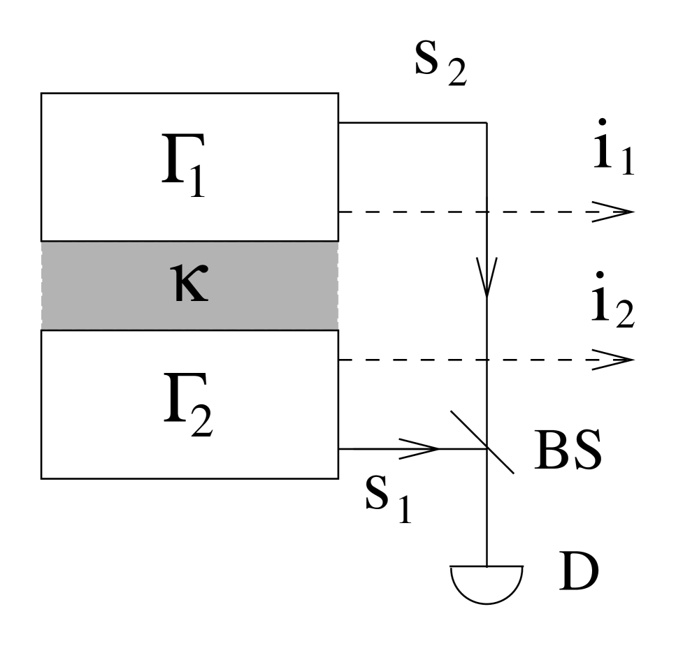
FIG. 1.: Experimental arrangement; gray color indicates the linear interaction region; BS – beamsplitter, D – detector.

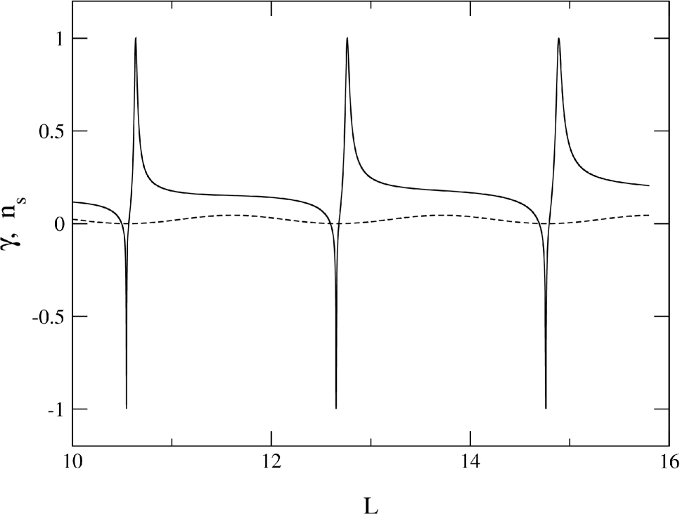
FIG. 2.: Mutual coherence of signal beams (solid line); mean total number of signal photons for the same interaction length $L$ (dotted line); $\kappa=3$, $\Gamma_{1}=0.1$, $\Gamma_{2}=0.3$.

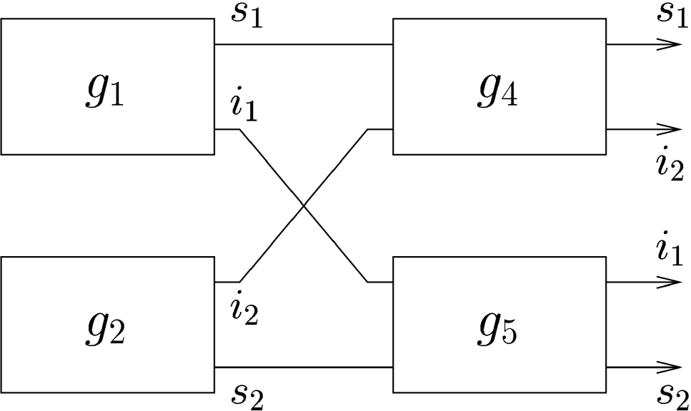
FIG. 3.: Substituting scheme for the two continuously coupled downconvertors shown in Fig. 1. Notice that the continuous interaction of three modes is replaced by a sequence of simpler devices at the expense of doubling the number of active elements.

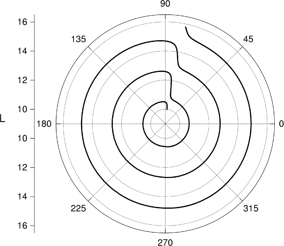
FIG. 4.: Mutual orientation of vectors ${\bf u}$ and ${\bf v}$ characterizing the substituting scheme of Fig. 3 which can substitute the continuously coupled device with $\kappa=3$, $\Gamma_{1}=0.1$, and $\Gamma_{2}=0.3$ (compare to Fig. 2).

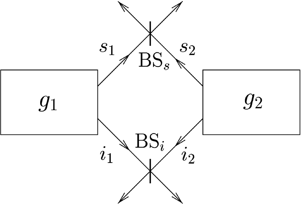
FIG. 5.: Substituting scheme for two continuously coupled downconvertors which is equivalent to the interferometer of Ou et al. Provided that all the input modes are in vacuum state, two downconvertors and two beamsplitters are enough to replace the original continuously coupled device.

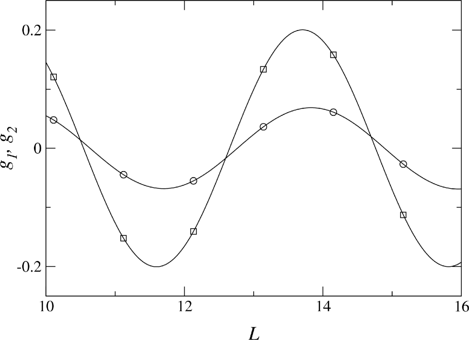
FIG. 6.: Parameters characterizing the substituting scheme (two-photon interferometer of Ou et al.) for two continuously coupled downconvertors. The coupling strengths of the original device are the same as in Figs. 2 and 4; $g_{1}$ (circles), $g_{2}$ (squares).

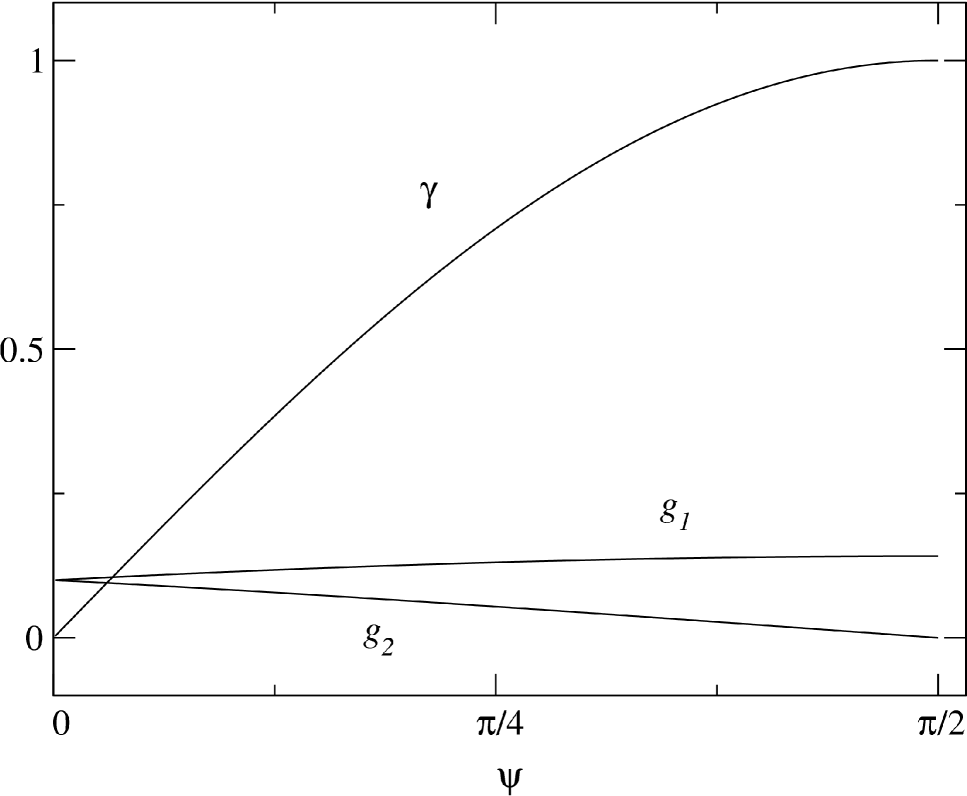
FIG. 7.: The two-photon interferometer of Ou et al. (Fig. 5) can simulate the experimental setup of Zou et al. (two downconvertors with aligned idler beams). The parameters characterizing the substituting scheme are shown as functions of the mixing angle of the beamsplitter controlling the alignment of idler beams in the experiment of Zou et al. ($\psi=\pi/2$ means perfect alignment); $r_{1}=r_{2}=0.1$.

REFERENCES

- [1] X. Y. Zou, L. J. Wang and L. Mandel, Phys. Rev. Lett. 67, 318 (1991); L. J. Wang, X. Y. Zou and L. Mandel, Phys. Rev. A 44, 4614 (1991).
- [2] G. Assanto , A. Laureti-Palma, C. Sibilia and M. Bertolotti, Opt. Commun. 110, 599 (1994); J. Janszky, C. Sibilia, M. Bertolotti, P. Adam and A. Petak, Quantum Semiclass. Opt. 7, 509 (1995); J. Peřina Jr. and J. Peřina in Progress in Optics, Vol. 41, edited by E. Wolf (Elsevier, Amsterdam, 2000).
- [3] Z. Y. Ou, L. J. Wang, X. Y. Zou, and L. Mandel, Phys. Rev. A 41, R566 (1990).
- [4] M. L. Stich and M. Bass, Laser Handbook (North–Holland, Amsterdam, 1985), Chapter 4; A. Yariv and P. Yeh, Optical Waves in Crystals (J. Wiley, New–York, 1984);
- [5] C. K. Hong and L. Mandel, Phys. Rev. A 31, 2409 (1985).
- [6] J. Řeháček, J. Peřina, P. Facchi, S. Pascazio, and L. Mišta Jr., Phys. Rev. A 62, 013804 (2001).
- [7] B. Misra and E. C. G. Sudarshan, J. Math. Phys. 18, 756 (1977); D. Home and M. A. B. Whitaker, Ann. Phys. 258, 237 (1997); P. Facchi and S. Pascazio in Progress in Optics, Vol. 41, edited by E. Wolf (Elsevier, Amsterdam, 2000).
- [8] A. Luis and J. Peřina, Phys. Rev. Lett. 76, 4340 (1996); A. Luis and L. L. Sánchez–Soto, Phys. Rev. A 57, 781 (1998).
- [9] E. Mihokova, S. Pascazio and L. S. Schulman, Phys. Rev. A56, 25 (1997).
- [10] J. Fiurášek and J. Peřina, Phys. Rev. A 62, 033808 (2000).
- [11] J. Wei and E. Norman, J. Math. Phys. 4, 575 (1963).
- [12] S. L. Braunstein, arXiv: quant-ph/9904002.
- [13] J. Řeháček and J. Peřina, Opt. Commun. 132, 549 (1996).
- [14] A. Peres, Am. J. Phys. 48, 931 (1980); K. Kraus, Found. Phys. 11, 547 (1981); P. Facchi and S. Pascazio, Phys. Rev. A 62, 023804 (2000).
- [15] L. S. Schulman, Phys. Rev. A57, 1059 (1998).