Quantum error-correcting codes associated with graphs

Abstract

We present a construction scheme for quantum error correcting codes. The basic ingredients are a graph and a finite abelian group, from which the code can explicitly be obtained. We prove necessary and sufficient conditions for the graph such that the resulting code corrects a certain number of errors. This allows a simple verification of the 1-error correcting property of fivefold codes in any dimension. As new examples we construct a large class of codes saturating the singleton bound, as well as a tenfold code detecting 3 errors.

I Introduction

From the beginning of Quantum Information Theory it was recognized that error correcting codes play a crucial role. On the one hand it was clear that without error correction decoherence effects could easily annihilate the gain in computing time promised by the new fast quantum algorithms. On the other hand, the no-cloning theorem [1] seemed to forbid at least the most naive approach to classical error correction for noisy channels, e.g., sending each bit three times and taking a majority vote at the output of the channel. Clearly, this simple scheme reduces classical errors with small probability of order $\varepsilon$ to order $\varepsilon^{2}$. The cloning required for sending ”the same bit” three times rules out direct quantum analogues of this scheme. It was therefore an important step to realize [2] that quantum mechanics had other, more subtle ways of “distributing” quantum information over several channels to stabilize against errors. One problem with the known schemes of quantum error correction (e.g. [3, 4]), however, is that they tend to be subtle indeed, and the verification of their error correcting capabilities often requires a lengthy computation. It is therefore desirable to find new, perhaps simpler ways of constructing error correcting codes, on which more direct intuitions might be built.

In this paper we propose a new scheme for constructing quantum error correcting codes, which has some of these advantages. The ingredients of our construction are a graph and a finite abelian group. The order of the group determines the type of systems for which errors are corrected so that, e.g., the two-element group corresponds to the qubit case (Compare [5, 6, 7, 8] for other constructions of non-binary codes). The number of vertices of the graph determines how many input systems are coded into how many output systems. From the edges of the graph one can then read off an explicit expression for the code. However, not every graph corresponds to a good code, and we will discuss the condition for the code to correct a certain number of errors. In the simplest case, the fivefold code [9, 10, 11] (for qubits as well as higher dimensional systems), it can be verified in a few lines that any two errors are corrected. We also give an example of a more complex tenfold code detecting 3 errors.

As we are going to discuss in a following paper in more detail, it turns out that the codes which can be achieved by our method are stabilizer codes. There are various efficient methods for constructing stabilizer codes [3, 4, 12, 13, 14, 15, 16]. However, we think that, compared to previous stabilizer constructions, our technique has some interesting new features.

• Often the condition for error correction can be proved for many groups simultaneously, so that one gets code families for systems of variable sizes.

• The geometric intuitions about graphs may become helpful for finding new constructions.

• Our codes have the property that in their natural basis all matrix elements of the coding operator have the same modulus (Hadamard form). This is prima facie opposite to the usual goal of getting as few non-zero matrix elements as possible. However, the latter can be achieved for our codes by a discrete Fourier transform applied to some channels. Moreover, the Hadamard form appears to be an interesting normal form for the codes which can be written in both ways.

• For some codes it is possible to exchange some input vertices with some output vertices, while retaining the error correction property. This kind of symmetry is much harder to see in the usual stabilizer constructions, and may prove to be helpful in coding problems with additional inputs and outputs, such as the internal state of the codig device in convolutional codes.

The paper is organized as follows: We begin by describing the general construction of the coding operator within Section II. In Section III we recapitulate the Knill-Laflamme condition for error correction and adapt it to our particular type of codes, resulting in a necessary and sufficient condition for a graph to generate a quantum error detecting code. The remaining sections contain examples of codes constructed in this way. In Section IV we show that it becomes simple indeed to verify the fivefold quantum codes. In Section V we demonstrate that for a given number $e$ of errors and number $k$ of inputs, there is a graph generating an infinite code family using $4e+k$ output systems, i.e., a family of codes saturating the singleton bound. Finally, in Section VI we construct a code with 1 input and 10 outputs, detecting 3 errors for arbitrary system size.

II Basic Construction

Every code we construct is completely determined by the follow ingredients:

• An undirected graph $\Gamma$ with two kinds of vertices.
  We distinguish the set $X$ of input vertices and the set $Y$ of output vertices. The links of the graph are given by the coincidence matrix of the graph, which we will denote by $\Gamma$ for short. Its matrix element $\Gamma({z_{1},z_{2}})$ is $1$ iff the vertices $z_{1},z_{2}\in(X\cup Y)$ are linked, and $0$ otherwise. More generally, we allow weighted graphs, whose incidence matrices have arbitrary integer entries, apart from the constraints $\Gamma({z_{1},z_{2}})=\Gamma({z_{2},z_{1}})$ and $\Gamma({z,z})=0$.

• A finite abelian group $G$ with a non-degenerate symmetric bicharacter.

By definition, a bicharacter is a function $\chi:G\times G\to{\mathbb{C}}$ such that $\chi(g+h,g^{\prime})=\chi(g,g^{\prime})\chi(h,g^{\prime})$ and a similar condition holds for the second argument, which is also implied by the assumed symmetry $\chi(g,g^{\prime})=\chi(g^{\prime},g)$. We also assume non-degeneracy in the sense that

$$\sum_{g}\chi(g,g^{\prime})=|G|\ \delta(g^{\prime})\equiv\left\{\begin{array}[]{rl}|G|&\text{for\ }g^{\prime}=0\\ 0&\text{for\ }g^{\prime}\neq 0\\ \end{array}\right.$$ (1)

Note that since every $g\in G$ has finite order, $\chi(g,g^{\prime})$ is always a root of unity, and $\overline{\chi(g,g^{\prime})}=\chi(-g,g^{\prime})$. For $G={\mathbb{Z}}_{p}$, the cyclic group of order $p$, the standard bicharacter is given by

$$\chi(g,h)=\exp\Bigl{(}\frac{2\pi i}{p}\;gh\Bigr{)}\;,$$ (2)

where $g,h$ are integers representing their class modulo $p$. Since every finite abelian group is a direct product of cyclic groups, this also shows the existence of bicharacters for any such group.

The input and output systems of the code are labeled by $X$ and $Y$. They are all of the same type, i.e., they are described by the same Hilbert space ${\cal H}=L^{2}(G)$. This is the space of all functions $\psi:G\to{\mathbb{C}}$ with scalar product $\langle\phi,\psi\rangle=|G|^{-1}\sum_{g}\overline{\phi}(g)\psi(g)$. For compactness of notation we write such normalized sums as integrals. Hence the scalar product becomes $\int{\rm d}g\ \overline{\phi}(g)\psi(g)$. The combined input system is thus described in the $|X|$-fold tensor product ${\cal H}^{\otimes X}=L^{2}(G^{X})$. Vectors in this space are functions of $|X|$ variables, one variable $g_{z}$ for every $z\in X$. The entire collection of variables will be denoted by $g^{X}$. The error correcting code will be an isometry

$${\bf v}_{\Gamma} : L^{2}(G^{X})\to L^{2}(G^{Y})$$ (3)

$$\bigl{(}{\bf v}_{\Gamma}\psi\bigr{)}(g^{Y}) = \int{\rm d}g^{X}\ {\bf v}_{\Gamma}[g^{X\cup Y}]\ \psi(g^{X})\;,$$ (4)

where ${\bf v}_{\Gamma}$ under the integral denotes the integral kernel of the operator ${\bf v}_{\Gamma}$. This kernel depends on both input and output variables, which are combined into a collection of variables $g_{z}$, one for each vertex $z\in X\cup Y$ of the graph. The core of our construction is an explicit expression for this integral kernel: apart from an overall normalization factor, it will simply be a product of phases, with each factor corresponding to a link of the graph:

$${\bf v}_{\Gamma}[g^{X\cup Y}]=|G|^{|X|/2}\ \prod_{\{z,z^{\prime}\}}\chi(g_{z},g_{z^{\prime}})^{\Gamma(z,z^{\prime})}\;,$$ (5)

where the product is over all $2$ element subsets ${\{z,z^{\prime}\}}\subset(X\cup Y)$. Thus for an ordinary graph (${\Gamma(z,z^{\prime})}=0,1$), this is the product of all $\chi(g_{z},g_{z^{\prime}})$, for which $z$ and $z^{\prime}$ are linked. The remarkable property of such codes is that apart from the normalization factor the kernel is everywhere of modulus $1$. When $G={\mathbb{Z}}_{p}$ is cyclic, and $\chi$ is given by Equation (2), we can write the phase in more compact form as

$${\bf v}_{\Gamma}[g^{X\cup Y}]=|G|^{|X|/2}\ \exp\Bigl{(}\frac{\pi i}{p}\;g^{X\cup Y}\cdot\Gamma\cdot g^{X\cup Y}\Bigr{)}\;,$$ (6)

where “$\cdot$” denotes the product of integer valued matrices and vectors. Note that every term in the sum $g^{X\cup Y}\cdot\Gamma\cdot g^{X\cup Y}$ occurs twice, which we compensated by a factor $1/2$.

This completes the construction of the operator ${\bf v}$ from the defining ingredients listed at the beginning of this section. Of course, in general this will not be an error correcting code nor even an isometry. The conditions for this will be studied in the following section.

III The condition for error correction

A general characterization of quantum error-correcting codes has first been worked out by E. Knill and R. Laflamme [17]. We briefly review here the main aspects, and adapt the condition the particular case of codes constructed as in the previous section. In this theory a quantum code is an isometry ${\bf v}:{\cal H}\to{\cal K}$ from the “input Hilbert space” ${\cal H}$ to the “output Hilbert space” ${\cal K}$. Thus an input density operator is transformed by coding into ${\bf v}\rho{\bf v}^{*}$, which is a density operator on ${\cal K}$. The output of the coding is then passed through a noisy channel. The noise is described by a certain class of errors, which are represented by a linear subspace ${\cal E}$ of operators on ${\cal K}$. The channel is thus represented by a completely positive linear map of the form

$${\bf T}(\rho)=\sum_{\alpha}F_{\alpha}\rho F_{\alpha}^{*}\;,$$ (7)

where $F_{\alpha}\in{\cal E}$. and are chosen such that the output is always normalized. The isometry ${\bf v}$ is said to be an error correcting code for ${\cal E}$, if there is a completely positive “recovery operator” ${\bf R}$ such that

$${\bf R}\bigr{(}{\bf T}({\bf v}\rho{\bf v}^{*})\bigr{)} = \rho$$ (8)

for all density operators on ${\cal H}$. By the theory of Knill and Laflamme [17] this is equivalent to the factorization condition

$$\ \langle{\bf v}\psi_{1},F_{\alpha}^{*}F_{\beta}{\bf v}\psi_{2}\rangle = \omega(F_{\alpha}^{*}F_{\beta})\ \langle\psi_{1},\psi_{2}\rangle$$ (9)

where $\omega(F_{\alpha},F_{\beta})$ is a factor independent of the arbitrary vectors $\psi_{1},\psi_{2}$. As in much of the literature on codes we will consider here a specific type of errors, namely errors happening only on a small number of outputs of the code. Thus the tensor product structure ${\cal H}^{\otimes Y}=L^{2}(G^{Y})$ of the output space becomes important. Let ${\mathfrak{A}}(E)$ denote the set of all operators on $L^{2}(G^{Y})$, which are localized in $E\subset Y$, i.e., which are the tensor product of an arbitrary operator on ${\cal H}^{\otimes E}$ with the identity on ${\cal H}^{\otimes Y\setminus E}$. We say that a code corrects $e$ errors, if $F_{\alpha},F_{\beta}$ in (9) may be chosen arbitrarily in the linear span of $\bigcup_{|E|\leq e}{\mathfrak{A}}(E)$. Note that the operators $F_{\alpha}^{*}F_{\beta}$ appearing in the scalar product (9) can then be localized on arbitrary sets of $2e$ elements and any operator with such localization may be written as a linear combination of such $F_{\alpha}^{*}F_{\beta}$. It is therefore convenient to introduce the following terminology: we say that the code ${\bf v}$ detects the error configuration $E\subset Y$, if

$$\ \langle{\bf v}\psi_{1},F{\bf v}\psi_{2}\rangle=\omega(F)\ \langle\psi_{1},\psi_{2}\rangle\;,$$ (10)

for all $F\in{\mathfrak{A}}(E)$. Then a code corrects $e$ errors, iff it detects all error configurations $E\subset Y$ with $|E|\leq 2e$.

We will now adapt these conditions to operators ${\bf v}_{\Gamma}$ of the special form (3). Consider a fixed error configuration $E\subset Y$, and let $I=Y\setminus E$. Then if $F$ is an operator $F$ on ${\cal H}^{\otimes E}$, with integral kernel $F[g^{E},h^{E}]$, the integral kernel of ${\bf v}^{*}F{\bf v}$ is

$${\bf v}_{\Gamma}^{*}F{\bf v}_{\Gamma}[g^{X},h^{X}] = \int{\rm d}g^{E}{\rm d}g^{I}{\rm d}h^{E}\ \overline{{\bf v}_{\Gamma}[g^{X},g^{E},g^{I}]}$$ (11)

$$\times F[g^{E},h^{E}]{\bf v}_{\Gamma}[h^{X},h^{E},g^{I}]\;.$$ (12)

This must be a multiple of the identity for every choice of $F$. Choosing, in particular, a rank one operator $F=|g^{E}\rangle\langle h^{E}|$ we find that error detection for the configuration $E$ is equivalent to the property that the correlation function

$${\bf w}_{[\Gamma,E]}[g^{X\cup E},h^{X\cup E}] := \int{\rm d}g^{I}\ \overline{{\bf v}_{\Gamma}[g^{X},g^{E},g^{I}]}$$ (13)

$$\times {\bf v}_{\Gamma}[h^{X},h^{E},g^{I}]$$ (14)

factorizes in the following manner

$${\bf w}_{[\Gamma,E]}[g^{X\cup E},h^{X\cup E}]=C(g^{E},h^{E})\ \delta(g^{X}-h^{X})\;,$$ (15)

where $\delta(g^{X})$ is defined to be $1$ if $g_{x}=0$ for all $x\in X$, and zero otherwise, and $C(g^{E},h^{E})$ is a factor independent of the input variables $g^{X},h^{X}$.

For two subsets $K,L$ of $X\cup Y$ we denote by $\Gamma^{K}_{L}$ the group homomorphism from $G^{L}$ to $G^{K}$ which can be derived from the corresponding submatrix of the incidence matrix $\Gamma$ by the prescription

$$\Gamma^{K}_{L}g^{L}:=\biggl{(}\sum_{l\in L}\Gamma(k,l)g_{l}\biggr{)}_{k\in K}\ \$$ (16)

and the following condition is necessary and sufficient for quantum error detection:

Theorem III.1

Given a finite abelian group $G$ and a weighted graph $\Gamma$ as in the basic construction. Then an error configuration $E\subset Y$ is detected by the quantum code ${\bf v}_{\Gamma}$ iff the system of equations

$$\Gamma^{I}_{X\cup E}d^{X\cup E}=0$$ (17)

with $I=Y\setminus E$ implies that

$$d^{X}=0\ \mbox{ and }\ \Gamma^{X}_{E}d^{E}=0\;.$$ (18)

The proof of Theorem III.1 is given in Appendix A and, in view of this result, we discuss some examples.

IV Example: The Fivefold Way

The first example of an optimal quantum error correcting code correcting all one bit errors was the famous five qubit code by [10]. The original code is not easy to verify, so it is gratifying to see that our construction produces such a code, which can be verified in a few lines. Moreover, our construction works simultaneously for all groups $G$, and is hence not restricted to qubits. Fivefold codes for higher dimensional systems have been constructed before [11], and if we believe a recent result by Rains [18], the qubit code is essentially unique anyway. Hence this section has mainly illustrative character.

Consider the graph in Figure 1 where the central vertex ”0” is the input vertex, and the remaining five are the output vertices.

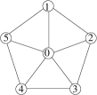
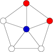
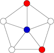
FIG. 1.: The left figure shows a graph for a fivefold code, where the central vertex is the input vertex. The two figures on the right side are the relevant 2-error configurations.

We will verify the condition of Theorem III.1 in a particularly strong form. Namely we will show that, for every 2-element error configuration $E$,

$$\Gamma^{I}_{X\cup E}d^{X\cup E}=0\qquad\text{implies}\qquad d^{X\cup E}=0\;.$$ (19)

The error configuration is a 2-element subset of the output vertices $1,...,4$, and for the purpose of verifying criterion (19) the input vertex 0 plays exactly the same role as an error. It is clear by symmetry that only the two configurations for $X\cup E$ shown by filled dots in Figure 1 need to be considered. Now the condition $\Gamma^{I}_{X\cup E}d^{X\cup E}=0$ is a set of equations, one for each “integration vertex” $y\in I$: For each vertex $y$ we have to sum the $d_{x}$ for all vertices of $x\in X\cup E$ connected to $y$, and equate to zero. (In a weighted graph, we would have to sum with coefficients given by the matrix $\Gamma$). The following is a table of equations arising in this way for the first error configuration, $X\cup E=\{0,1,2\}$:

Vertex $y$	Equation
3	$d_{0}+d_{2}=0$
4	$d_{0}=0$
5	$d_{0}+d_{1}=0$

Clearly, this implies $d_{0}=d_{1}=d_{2}=0$ in any abelian group. Similarly, for the second error configuration $X\cup E=\{0,1,3\}$we get the equations

Vertex $y$	Equation
2	$d_{0}+d_{1}+d_{3}=0$
4	$d_{0}+d_{3}=0$
5	$d_{0}+d_{1}=0$

which once again implies $d_{0}=d_{1}=d_{2}=0$. This concludes the verification that the code associated with the graph in Figure 1, and an arbitrary finite abelian group $G$, detects any two errors, hence corrects one error.

In fact, we proved a little bit more than that. The essential part of the proof was to look at certain $3\times 3$-submatrices of the $6\times 6$-matrix $\Gamma$, namely those corresponding to an off-diagonal block in the partition of the vertices $\{0,1,\ldots,5\}$ into two disjoint subsets $X\cup E$ and $I$, and to show that each such submatrix is non-singular. Regarded in this way, it becomes irrelevant to which of the two sets in the partition the input vertex “$0$” belongs, so we showed that any vertex, even a peripheral one, may be taken as input vertex, and we still get a 1-error correcting code.

This may seem like a rather strong property of the graph we chose. However, there is (exactly) one other graph with six vertices, which produces in the same way a 1-error correcting code for arbitrary choice of input vertex and abelian group $G$. This is shown in Figure2.

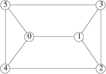
FIG. 2.: An alternative graph for a fivefold code which corrects one error.

V Codes saturating the singleton bound

In this Section we briefly discuss one natural generalization of the idea emerging in the previous section. For definiteness, let us fix $G$ as a cyclic group of prime order $d$, so ${\mathbb{Z}}_{d}$ is a field, and choose an integer $m$. We then ask for symmetric $2m\times 2m$-matrices $\Gamma$ with integer entries (or, equivalently, entries in ${\mathbb{Z}}_{d}$) with the following property: for any $m$-element subset $I\subset\{1,\ldots,2m\}$ the $m\times m$-submatrix $\Gamma_{ij}$ with $i\in I,j\notin I$ is invertible in the field ${\mathbb{Z}}_{d}$. For the purpose of this section, let us call such a matrix strongly error correcting for the prime number $d$.

What codes can we get from such matrices? Just as in the previous section, let us specify any set $X$ of $k<m$ vertices as input vertices, and call the remaining $n=(2m-k)$ ones output vertices. Then for any configuration of $e=m-k$ errors, the set $X\cup E$ and its complement $I$ will have exactly $m$ elements. By assumption, the strong form of the error correcting condition (19) is satisfied, hence the code detects $e$ errors. These parameters satisfy

$$n=2e+k\;,$$ (20)

i.e., the general inequality $n\leq 2e+k$, known as the singleton bound [17] is satisfied with equality for any such code.

How can one get strongly error correcting matrices $\Gamma$ in a practical way? Here is a procedure, we found easy to work with for small $m$, using a symbolic algebra program. First, we introduce variables for each matrix element $\Gamma_{ij}$ with $i>j$, and compute the determinants of all off-diagonal $m\times m$-submatrices as symbolic expressions in these variables. As we go along fixing integer values for these $\Gamma_{ij}$, the determinant expressions become simpler, and in some cases factorize. Each of these factors has to be kept non-zero by the next choice of a $\Gamma_{ij}$-value. Finally, we end up with an integer matrix, whose off-diagonal $m\times m$-submatrices all have non-zero integer determinant. Then, for any prime $d$, which does not divide any of these integers, we have solved the problem.

It is natural to begin this process by setting as many weights as possible equal to zero. It is easy to see that Theorem III.1 does not allow too many $\Gamma(k,l)=0$ because an entire row of zeros in the matrix $\Gamma^{I}_{X\cup E}$ leaves one of the difference variables unconstrained. Similarly, in the condition for strong error correction it is clear that no off-diagonal submatrix should have a row of zeros, i.e., each one of the $2m$ vertices must be connected to at least $m$ other vertices. The graph in Figure 3 is as sparse as possible under these constraints ($m=4$), and was the starting point for a search for non-zero weights, as described above, resulting in the matrix

$$\Gamma=\left(\begin{array}[]{cccccccc}0&0&1&0&1&1&1&0\\ 0&0&0&1&1&1&0&1\\ 1&0&0&0&2&0&-1&1\\ 0&1&0&0&0&1&2&-2\\ 1&1&2&0&0&0&-2&0\\ 1&1&0&1&0&0&0&-1\\ 1&0&-1&2&-2&0&0&0\\ 0&1&1&-2&0&-1&0&0\end{array}\right)\ \ .$$ (21)

This matrix can either be used to get codes detecting three errors on an arbitrarily chosen single input vertex, or as a code detecting two errors (or correcting 1) on two arbitrarily chosen inputs. The set of determinants is $\{-11,-8,-5,-4,-2,-1,1,2,4,5,8,9\}$, so this will work for any prime $d$ not in in the set $\{2,3,5,11\}$. By fixing the choice of the input vertices, we may restrict to a smaller set of partitions (the input vertices always belong to the same set), hence we get fewer constraints. For example, the code with input vertices $\{1,2\}$ has no relevant subdeterminant containing a factor $3$, so the resulting code corrects one error on arbitrary pairs of $3$-level systems.

Within the above example, the number of matrix elements set to zero is maximal, namely $\nu_{i}=4$ for each row $i=1,\cdots,8$. Looking at the corresponding graph, $\nu_{i}=4$ is just the number of lines meeting a particular vertex as one can see from Figure 3.

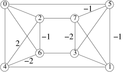
FIG. 3.: Graphical representation of the weighted graph in Equation (19). Edges without label have weight $1$.

Strongly error correcting matrices exist in any dimension, so the code parameters saturating the singleton bound (20) can be chosen arbitrarily, if the dimension $d$ of the one-site system is taken to avoid a certain finite set of primes (Compare also [5]). The argument is quite simple: consider the $m\times m$- subdeterminants of symmetric $2m\times 2m$-matrices as a family of polynomials $f_{\alpha}$, $\alpha=1,\cdots,{2n\choose n}$ in ${2n\choose 2}$ variables. None of these vanishes identically and since ${\mathbb{Z}}$ is an integral domain, which in contrast is wrong for finite fields, the product polynomial $\prod_{\alpha}f_{\alpha}\not=0$ is non zero [19, p. 106]. This implies that there exists an integer tuple $\Gamma$ of arguments that $\prod_{\alpha}f_{\alpha}(\Gamma)\not=0$. Thus we have shown the following statement:

Proposition V.1

For each number $e$ of errors, there exists a prime $d$ and a weighted graph $\Gamma$ such that the quantum code, associated with the weighted graph $\Gamma$, is a quantum error correcting code, which encodes $k$ $d$-level systems into $4e+k$ $p$-level systems, and which corrects $e$ errors.

VI A 10-fold quantum error-detecting code

In this section we present more complex example for a graph, which yields for every finite abelian group $G$ a 10-bit code, detecting 3 errors is given by Figure 4. At the first look, this graph looks rather complicated, but it can be described in a simple fashion, by looking at the graph for the fivefold code in Figure 1.

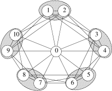
FIG. 4.: The graph for a tenfold code.

Namely, the graph, given by Figure 4, can be obtained as follows: The output vertices $\{1,2,3,4,5\}$ of the graph in Figure 1 are replaced by pairs: $1\mapsto\{1,2\}$, $2\mapsto\{3,4\}$, …, $5\mapsto\{9,10\}$. Each output vertex is connected with the following vertices: The central input vertex $0$, the vertex belonging the same pair, and all output vertices belonging to neighbored pairs.

The symmetry of this graph can efficiently be used to check that each error configuration with 3 errors can be detected. As it is depicted by Figure 5, there are only four 3-error configurations to distinguish:

• All errors occur within different pairs and all these pairs are neighbored (first graph in Figure 5).

• All errors occur within different pairs and only two of these pairs are neighbored (second graph in Figure 5).

• One pair is totally affected by errors and the remaining error occurs within a pair which is not neighbored (third graph in Figure 5).

• One pair is totally affected by errors and the remaining error occurs within a neighbored pair (4th graph in Figure 5).

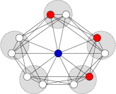
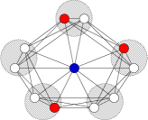
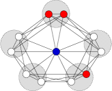
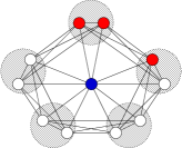
FIG. 5.: A complete family of inequivalent error configurations for the graph in Fig. 3.

Proposition VI.1

For each finite abelian group $G$, the quantum code, which is associated with the graph given by Figure 5, is a quantum error-detecting code, encoding 1 input system into 10 output systems and detecting 3 errors.

Proof: Suppose that each error occurs in different pairs and all these pairs are neighbored (first graph in Figure 5), e.g. the error configuration $\{1,3,5\}$. Then we proceed as in the example for the fivefold code to obtain the system of equation (17):

Vertices $y$	Equation
2	$d_{0}+d_{1}+d_{3}=0$
4	$d_{0}+d_{1}+d_{3}+d_{5}=0$
6	$d_{0}+d_{3}+d_{5}=0$
7 and 8	$d_{0}+d_{5}=0$
9 and 10	$d_{0}+d_{1}=0$

and we conclude that $d_{0}=0$ and $d_{1}+d_{3}+d_{5}=0$ are true. Thus the equations (18) are fulfilled and the corresponding error configuration is detected.

Analogously, one checks that each error configuration, where each error occurs in a different pair and only two of these pairs are neighbored (second graph in Figure 5) is also detected.

We now consider an error configuration, where one pair $\{1,2\}$ is totally corrupted and the remaining error vertex, e.g. $5$, is contained within a non-neighbored pair (third graph in Figure 5). We obtain for the system of equations (17):

Vertices $y$	Equation
3 and 4	$d_{0}+d_{1}+d_{2}+d_{5}=0$
6, 7 and 8	$d_{0}+d_{5}=0$
9 and 10	$d_{0}+d_{1}+d_{2}=0$
7 and 8	$d_{0}+d_{5}=0$

and we conclude again that $d_{0}=0$ and $d_{1}+d_{2}+d_{5}=0$ is true. The equations (18) are fulfilled which implies that the corresponding error configuration is also detected.

Finally, it is a bit more straightforward as in the previous case to show that an error configuration, where two errors occur within one pair and the remaining error within a neighbored pair (4th graph in Figure 5) is detected. $\square$

VII Conclusion and outlook

In this paper we had to limit the exploration of our construction scheme to a few examples. A more systematic investigation is, of course, under way. Some of the issues in this investigation are the following.

• We already mentioned that all codes constructed from graphs are stabilizer codes. This is verified by explicitly constructing a group of unitaries, composed out of shifts and multiplication by characters, leaving all vectors in the code space invariant. The converse of this statement is not so clear, i.e., how to embed the usual stabilizer code constructions into our scheme, and to characterize the subset of codes for which this is possible.

• We have seen in Sec. IV that different graphs generate 5-qubit codes, although such codes are presumably unique up to local transformations. It would be helpful to characterize the local unitary transformations taking one graph code into another, and to study the relationships between the resulting graphs. The Rains invariants [20, 21, 22] for graph codes can be computed relatively easily, and should help to decide such isomorphism issues.

• From Sec. V it is clear that the singleton bound becomes easier and easier to satisfy as the dimension $d$ of the single system Hilbert space increases. This suggests the search for bounds describing the resource limitations in coding more adequately, perhaps by taking into account more detailed features of the error syndromes than just the maximal number of errors. Our construction could be helpful for developing and testing such bounds.

• Non-stabilizer quantum codes can be constructed from families of stabilizer codes by taking their union [23], where one has to require that the protected subspaces, corresponding to the codes within the family, are mutually orthogonal and that this property remains valid after error operations. Examples of such non-stabilizer codes are given in [24, 25]. In view of our construction scheme, it would be desirable to find sufficient conditions for a family of graphs such that the union of their corresponding graph codes yields a (possibly more efficient) non-stabilizer code.

Acknowledgment:

We would like to thank Mary Beth Ruskai for helpful discussions and for supporting this investigation with many ideas. Funding by the European Union project EQUIP (contract IST-1999-11053) is gratefully acknowledged.

A

Proof of Theorem III.1: We first compute the function ${\bf w}_{[\Gamma,E]}$, defined by (13). It is convenient to introduce for two subsets $K,K^{\prime}$ of $X\cup Y$ the expression

$$\chi^{\Gamma}(g^{K},g^{K^{\prime}}):=\prod_{\{k,k^{\prime}\}:k\in K,k^{\prime}\in K^{\prime}}\chi(g_{k},g_{k^{\prime}})^{\Gamma(k,k^{\prime})}$$ (A1)

where the product is taken over all two elementary sets with one element taken from $K$ and the other taken from $K^{\prime}$. Hence the factor for $\{k,k^{\prime}\}=\{k^{\prime},k\}$ only occurs once within the product. Now we write the integrand in (13) as a product of two terms

$$\hskip-25.0pt\overline{{\bf v}_{\Gamma}[g^{X},g^{E},g^{I}]}{\bf v}_{\Gamma}[h^{X},h^{E},g^{I}]$$ (A2)

$$= |G|^{|X|}{\chi^{\Gamma}(h^{X\cup E},h^{X\cup E})\over\chi^{\Gamma}(g^{X\cup E},g^{X\cup E})}{\chi^{\Gamma}(h^{X\cup E},g^{I})\over\chi^{\Gamma}(g^{X\cup E},g^{I})}\ \ .$$ (A3)

Here only the last factor on the right hand side depends on the integration variables $g^{I}$ associated with the set $I=Y\setminus E$. In order to carry out the integral over one variable $g_{i}$, $i\in I$, we select the $g_{i}$ dependent part out of $\chi^{\Gamma}(h^{X\cup E},g^{I})$, which is

$$\prod_{\{z,i\}:z\in X\cup E}\chi(h_{z},g_{i})^{\Gamma(z,i)}\ \ .$$ (A4)

Analogously the $g_{i}$ dependent part of $\chi^{\Gamma}(g^{X\cup E},g^{I})$ is the same expression with $h$ replaced by $g$. Thus the $g_{i}$ dependent part of (A2) is

$$\prod_{\{z,i\}:z\in X\cup E}\chi(g_{z},g_{i})^{-\Gamma(z,i)}\chi(h_{z},g_{i})^{\Gamma(z,i)}\ \ .$$ (A5)

Using the character property of $\chi(\cdot,g_{i})$ we can simplify this to a single factor of the form $\chi(k,g_{i})$. Explicitly,

$$k=\sum_{j\in X\cup E}\Gamma_{ij}(h_{j}-g_{j})\;,$$ (A6)

and this sum contains none of the variables associated with $I$, because $I\cap(X\cup E)=\emptyset$. The integral over $g_{i}$ then gives $\delta(k)$, and we find

$$\hskip-15.0pt{\bf w}_{[\Gamma,E]}[g^{X\cup E},h^{X\cup E}]$$ (A7)

$$= |G|^{|X|}{\chi^{\Gamma}(h^{X\cup E},h^{X\cup E})\over\chi^{\Gamma}(g^{X\cup E},g^{X\cup E})}\ \delta(\Gamma^{I}_{X\cup E}(h^{X\cup E}-g^{X\cup E}))\ \ .$$ (A8)

Our task is to establish the necessary and sufficient conditions for this to be of the form

$$C(g^{E},h^{E})\ \delta(h^{X}-g^{X})\;,$$ (A9)

required by Eq.(15).

Now the expression (A7) has the required property of vanishing except for $g^{X}=h^{X}$ if and only if this is already implied by the vanishing of the $\delta$-function in (A7), i.e., if and only $d^{X}\neq 0$ implies $\Gamma^{I}_{X\cup E}(d^{X\cup E})\neq 0$. This is the first part of the condition in Theorem III.1.

From now on we assume, as we may, that $\Gamma^{I}_{X\cup E}(d^{X\cup E})=0$ implies $d^{X}=0$. Then the dependence of (A7) on the input variables $g^{X}$ and $h^{X}$ can be simplified. The $\delta$-function can be written as

$$\hskip-30.0pt\delta\bigl{(}\Gamma^{I}_{X\cup E}(h^{X\cup E}-g^{X\cup E})\bigr{)}$$ (A10)

$$= \delta\bigl{(}\Gamma^{I}_{E}(h^{E}-g^{E})\bigr{)}\ \delta(h^{X}-g^{X})\;,$$ (A11)

because the two expressions are equal for $h^{X}=g^{X}$, and for $h^{X}\neq g^{X}$ they both vanish by assumption.

To simplify the bicharacter quotient in (A7), we use Eq. (A1) to write

$$\hskip-30.0pt\chi^{\Gamma}(h^{X\cup E},h^{X\cup E})$$ (A12)

$$= \chi^{\Gamma}(h^{X},h^{X})\chi^{\Gamma}(h^{E},h^{X})\chi^{\Gamma}(h^{E},h^{E})\;.$$ (A13)

With a similar decomposition of $\chi^{\Gamma}(g^{X\cup E},g^{X\cup E})$ we use the condition that, wherever the $\delta$-function in (A7) is non-zero, we have $g^{X}=h^{X}$. Hence the $X-X$ factors cancel, and we can write the quotient of the $X-E$-terms as

$${\chi^{\Gamma}(h^{E},h^{X})\over\chi^{\Gamma}(g^{E},h^{X})}=\prod_{j\in X}\chi\bigl{(}\sum_{i\in E}\Gamma_{ji}(h_{i}-g_{i}),h_{j}\Bigr{)}.$$ (A14)

For (A7) to be of the desired form (A9) with $C(g^{E},h^{E})$ independent of the $X$-variables, this expression must be independent of all $h_{j},j\in X$, whenever $\delta\bigl{(}\Gamma^{I}_{E}(h^{E}-g^{E})\bigr{)}\neq 0$. But (A14) is independent of $h_{j}$ if and only if $\sum_{i}\Gamma_{ji}(h_{i}-g_{i})=0$. Hence we must have that $\Gamma^{I}_{E}(h^{E}-g^{E})=0$ implies $\Gamma^{X}_{E}(h^{E}-g^{E})=0$. This is the second condition from Theorem III.1, which we have thus shown to be necessary. Conversely, it is sufficient to ensure that (A14) is equal to $1$, and (A7) has the desired form (A9) with

$$C(g^{E},h^{E}):=|G|^{|X|}{\chi^{\Gamma}(h^{E},h^{E})\over\chi^{\Gamma}(g^{E},g^{E})}\ \delta(\Gamma^{I}_{E}(h^{E}-g^{E})).$$ (A15)

This concludes the proof.

REFERENCES

- [1] Wootters, W. K. and Zurek, W. H.: A single quantum cannot be cloned. Nature 299, 802-803, (1982)
- [2] Calderbank, A.R. and Shor P. W.: Good quantum error-correcting codes exists. Phys. Rev. A 54, 1098, (1996)
- [3] Calderbank, A.R., Rains, E.M., Shor, P.W., and Sloane, N.J.A.: Quantum error correction and orthogonal geometry. Phys. Rev. Lett. 78, (1997), 405-408
- [4] Calderbank, A.R., Rains, E.M., Shor, P.W., and Sloane, N.J.A.: Quantum error correction via codes over GF(4). IEEE Transactions on Information Theory, quant-ph/9608006
- [5] Knill, E.: Non-binary unitary error bases and quantum codes Los Alamos National Laboratory Report LAUR-96-2717, (1996)
- [6] Rains, E.M.: Nonbinary quantum codes. quant-ph/9703048
- [7] Matsumoto, R. and Uyematsu, T.: Constructing quantum error correcting codes for -state systems from classical error correcting codes. IEICE Transactions on Fundamentals of Electronics, Communications and Computer Sciences, vol. E83-A, no.10, Oct 2000
- [8] Ashikhmin, A. and Knill, E.: Nonbinary quantum stabilizer codes. quant-ph/0005008
- [9] Bennet, C.H., DiVincenzo, D.P., Smolin, J.A., and Wootters, W.K.: Mixed state entanglement and quantum error correction. Phys. Rev. A 54, 3824, (1996)
- [10] Laflamme, R., Miquil, C., Paz, J.-P., Zurek, W.H.: Perfect quantum error correction code Phys. Rev. Lett. 77, 198, (1996)
- [11] Chau, H.F.: Five quantum register error correcting code for higher spin systems. quant-ph/9702033
- [12] Gottesman, D.: Class of quantum error-correcting codes saturating the quantum Hamming bound. Phys. Rev. A 54, 1862, (1996)
- [13] Gottesman, D.: Stabilizer codes and quantum error correction. PhD thesis (1997)
- [14] Grassl, M. and Beth, T.: Quantum BCH codes Proceedings X. International Symposium on Theoretical Electrical Engineering, Magdeburg 1999
- [15] Grassl, M. and Beth, T.: Cyclic quantum error-correcting codes quant-ph/9910061
- [16] Grassl, M., Geiselmann, W., and Beth, T.: Quantum Reed-Solomon codes In Proceedings AAECC-13, 1999
- [17] Knill, E. and Laflamme, R.: Theory of quantum error-correcting codes. Phys. Rev. A 55, 900, (1997)
- [18] Rains, E.M.: Quantum codes of minimum distance two. quant-ph/9704043
- [19] Jacobson, N.: Lectures in abstract algebra. Vol I. Basic concepts, Springer, New York, Heidelberg, Berlin, (1964)
- [20] Rains, E.M.: Quantum weight enumerators. quant-ph/9612015
- [21] Rains, E.M.: Quantum shadow enumerators. quant-ph/9611001
- [22] Rains, E.M.: Polynomial invariants of quantum codes. quant-ph/9704042
- [23] Grassl, M. and Beth, T.: A note on non-additive quantum codes quant-ph/9703016
- [24] Rains, E.M., Hardin, R.H., Shor, P.W., and Sloane, N.J.A.: A non-additive quantum code. quant-ph/9703002
- [25] Ruskai, M.B.: Pauli exchange and quantum error correction. quant-ph/0006008