Finding cliques by quantum adiabatic evolution

Abstract

Quantum adiabatic evolution provides a general technique for the solution of combinatorial search problems on quantum computers. We present the results of a numerical study of a particular application of quantum adiabatic evolution, the problem of finding the largest clique in a random graph. An $n$-vertex random graph has each edge included with probability $1\over 2$, and a clique is a completely connected subgraph. There is no known classical algorithm that finds the largest clique in a random graph with high probability and runs in a time polynomial in $n$. For the small graphs we are able to investigate ($n\leq 18$), the quantum algorithm appears to require only a quadratic run time.

MIT-CTP #3067

I Introduction

Quantum computation has been shown to have advantages in solving some problems that require searching through a large space, but the exact nature of this advantage remains an important open question. In this paper, we explore quantum adiabatic evolution, a general technique for solving such problems. Specifically, we consider the application of quantum adiabatic evolution to the problem of finding the largest clique in a random graph.

Quantum adiabatic evolution provides a natural framework for solving combinatorial search problems on quantum computers [1, 2]. The Hamiltonian which governs the evolution of the quantum system interpolates smoothly between an initial Hamiltonian whose ground state is easy to construct and a final Hamiltonian whose ground state encodes the desired solution. The evolution of the quantum state proceeds in continuous time according to the Schrödinger equation, starting in the ground state of the initial Hamiltonian. If the Hamiltonian varies slowly enough, the evolution will closely track the instantaneous ground state and end in a state close to the desired, final ground state. Any problem which can be recast as the minimization of an energy function (which can then be converted into a quantum Hamiltonian) can potentially be solved in this way. The key question is how much time is required for the evolution to produce a final state that gives a reasonable probability of finding the solution.

Previous work along these lines has focused on satisfiability problems, in which the goal is to find an assignment of Boolean variables that makes a certain logical expression over those variables true. Early work demonstrated that certain easy problems could in fact be solved efficiently by adiabatic evolution [1]. More general problems have been treated numerically, and studies of a set of Exact Cover instances designed to be hard have shown polynomial behavior out to instances containing as many as twenty bits [3, 4]. However, for satisfiability problems like Exact Cover or 3-SAT, there are many ways to generate random instances, and in general the observed performance of an algorithm depends on the exact scheme chosen.

In this paper, we try to extend our understanding of the quantum adiabatic evolution technique by studying its application to the problem of finding the largest clique in a random graph. There is a natural way to generate random graphs, and for this distribution it is generally believed that no polynomial-time classical algorithm will succeed in finding the largest clique with high probability. Thus an efficient quantum algorithm for this problem would be an important step towards revealing the true power of quantum computers. Unfortunately, asymptotic analysis of quantum adiabatic evolution algorithms appears to be difficult.

Here, we present a numerical study of our quantum adiabatic evolution algorithm for finding cliques in graphs. We first review adiabatic evolution in general and discuss the properties of cliques in random graphs. After showing how adiabatic evolution may be used to find cliques in any graph, we present data showing that the median time required by the algorithm to find the largest clique in a random graph apparently grows quadratically for graphs of up to eighteen vertices. We then focus on graphs containing fifteen vertices and show that the algorithm behaves well for the 8000 random graphs we generate. It is possible that these results on small graphs capture the asymptotic behavior of the algorithm, giving some further evidence that quantum computation by adiabatic evolution may be a good technique for solving hard combinatorial search problems.

II Quantum computation by adiabatic evolution

Aside from measurements, a quantum system with the time-dependent Hamiltonian $H(t)$ evolves according to the Schrödinger equation,

$$i{\partial\over\partial t}|\psi(t)\rangle=H(t)|\psi(t)\rangle$$ (1)

(we set $\hbar=1$ throughout). If $H(t)$ varies sufficiently slowly, and if its instantaneous energy levels do not cross as a function of time, then the quantum adiabatic theorem says that the evolution will track the instantaneous eigenstates [5]. More specifically, suppose that we wish to evolve from $t=0$ to $t=T$, the run time, and that we have a one-parameter family of Hamiltonians $\tilde{H}(s)$ that varies smoothly for $0\leq s\leq 1$. We set $H(t)=\tilde{H}(t/T)$ so that the run time $T$ governs how slowly $H$ varies. Let

$$\tilde{H}(s)|j,s\rangle=E_{j}(s)|j,s\rangle$$ (2)

denote the instantaneous eigenstates of $\tilde{H}(s)$ with energy eigenvalues $E_{j}(s)$ arranged in nondecreasing order. Assume that $E_{0}(s)\neq E_{1}(s)$ for all $0\leq s\leq 1$, so that there is always a positive energy gap between the ground and first excited states. Time evolution according to (1), starting in the initial ground state $|\psi(0)\rangle=|0,s=0\rangle$, produces a final state $|\psi(T)\rangle$. The adiabatic theorem says that in the limit $T\to\infty$, $|\psi(T)\rangle$ is the final ground state $|0,s=1\rangle$ (up to a phase).

Now imagine that the solution to an interesting computational problem can be characterizing as minimizing a particular energy function. This means we can construct a Hamiltonian $H_{P}$ (the problem Hamiltonian) which is diagonal in the computational basis and whose ground state encodes the solution to the problem. The quantum adiabatic theorem yields an idea for a way to construct this ground state. Suppose we have another Hamiltonian $H_{B}$ (the beginning Hamiltonian) whose ground state — perhaps a uniform superposition over all possible solutions to the problem — is easy to construct. If we choose the interpolating Hamiltonian

$$\tilde{H}(s)=(1-s)H_{B}+sH_{P}\,,$$ (3)

so that

$$H(t)=\left(1-{t\over T}\right)H_{B}+{t\over T}H_{P}\,,$$ (4)

then evolution from $t=0$ to $t=T$ starting in the ground state of $H_{B}$ will, in the adiabatic limit, produce the ground state of $H_{P}$, thus giving the solution to the problem.

Of course, computation which takes an infinite amount of time is of little practical value. In practice, we would like to find a reasonably small value of $T$ such that the final state gives us a reasonable chance of finding the solution to the problem. This time can be characterized in terms of the spectrum of $\tilde{H}(s)$. Let

$$g=\min_{0\leq s\leq 1}\left(E_{1}(s)-E_{0}(s)\right)$$ (5)

denote the minimum gap over all values of $s$ between the ground state and the first excited state, and let

$${\cal E}=\max_{0\leq s\leq 1}|\langle 1,s|{\partial\tilde{H}\over\partial s}|0,s\rangle|$$ (6)

denote the most rapidly changing matrix element between the ground and first excited state. Then choosing

$$T\gg{{\cal E}\over g^{2}}$$ (7)

suffices to produce a final state arbitrarily close to the desired ground state. In typical problems of interest, $\cal E$ will scale polynomially with the problem size, so the efficiency of the algorithm hinges on whether $g$ is exponentially small or not. Unfortunately, the size of this gap is generally difficult to estimate analytically.

III Large cliques in random graphs

Here, we review some simple graph-theoretic definitions. For our purposes, a graph $G$ is an $n\times n$ binary matrix that describes the connectivity of a set of $n$ vertices labeled by the integers $1$ through $n$. The matrix element $G_{ij}$ is $1$ if vertices $i$ and $j$ are connected by an edge and $0$ if they are not. A random graph is a graph in which each pair of vertices is connected, independently, with probability $1\over 2$. A clique is a subgraph in which every pair of vertices is connected by an edge. In other words, $S\subseteq\{1,\ldots,n\}$ is a clique in $G$ iff $G_{ij}=1$ for all $i,j\in S$, $i\neq j$.

Many interesting properties of random graphs have been discovered since their introduction by Erdös and Réyni [6]. For a survey of such results, see [7], and for a review of algorithms related to random graphs, see [8]. In particular, we are interested in algorithms for finding large cliques in random graphs. Roughly speaking, the largest clique in a random graph with $n$ vertices has about $2\log n$ vertices (all logs are base 2). In fact, given $n$, there is an integer $d(n)\approx 2\log n$ such that the largest clique has size $d(n)$ or $d(n)+1$ with probability tending to 1 as $n\to\infty$ [9].

No polynomial time algorithm is known that will find, with high probability, cliques of size $(1+\epsilon)\log n$ for any $\epsilon>0$. A simple greedy heuristic will only produce cliques of size $1\cdot\log n$ in polynomial time. Jerrum has analyzed in detail a more sophisticated technique based on the Metropolis method, and he shows that it can require super-polynomial time to find cliques larger than $\log n$ [10]. Indeed, it has been conjectured that no efficient algorithm will find large cliques, and this conjecture forms the basis of a proposed cryptographic protocol [11]. Our goal, then, is to investigate the possibility of an efficient quantum algorithm which will find the largest clique in a random graph.

IV Algorithm

We now present an algorithm based on quantum adiabatic evolution for finding cliques in graphs. This algorithm finds cliques of a particular size $k$. Since random graphs asymptotically have a maximal clique with one of two known sizes, it suffices to have a good algorithm for finding cliques of a particular size.

The basis states in our Hilbert space will represent subsets of the set of vertices $\{1,\ldots,n\}$. Let the computational basis state $|z\rangle=|z_{1}\ldots z_{n}\rangle$, where each $z_{i}=0$ or $1$, represent the subset which includes vertex $i$ iff $z_{i}=1$. Since we are only interested in subsets of size $k$, we may restrict ourselves to the $n\choose k$-dimensional subspace spanned by states $|z\rangle$ for which $h(z)=k$, where $h(z)$ denotes the Hamming weight of $z$ (the number of ones that appear in its binary representation $z_{1}\ldots z_{n}$).

Our beginning Hamiltonian is

$$H_{B}=-\sum_{i>j}^{n}S^{ij}\,,$$ (8)

where

$$S^{ij}=\left(\matrix{0&0&0&0\cr 0&0&1&0\cr 0&1&0&0\cr 0&0&0&0}\right)^{ij}$$ (9)

acts on qubits $i$ and $j$ in the basis $\{|00\rangle,|01\rangle,|10\rangle,|11\rangle\}$. Note that $S^{ij}$ generates a swap between the $i$th and $j$th qubits. In the subspace of states of Hamming weight $k$ this Hamiltonian has the ground state

$$|\psi_{0}\rangle={n\choose k}^{-1/2}\sum_{h(z)=k}|z\rangle\,,$$ (10)

a uniform superposition of all states of Hamming weight $k$. This is the initial state for the algorithm. It can be prepared efficiently from the $|0\rangle$ state, as we describe in detail in the following section.

The problem Hamiltonian is diagonal in the computational basis:

$$H_{P}|z\rangle=\sum_{i>j}(1-G_{ij})z_{i}z_{j}|z\rangle\,.$$ (11)

In other words, every pair of vertices that are in the state $|z\rangle$ but are not connected in the graph raises the energy by one unit. Thus the ground state of this Hamiltonian (in the subspace of states of Hamming weight $k$) will be a state with all $k$ vertices connected in the graph, assuming such a state exists.

To summarize the algorithm, we prepare the system in the state given by (10) and evolve according to the Hamiltonian (4), where $H_{B}$ is given by (8) and $H_{P}$ is given by (11). If there is a unique clique of size $k$, adiabatic evolution will yield the corresponding state, which can easily be checked to verify that it is indeed a clique. If there are multiple cliques of size $k$, we will find some superposition of the corresponding states, so that measurement will give each of the various cliques with some probability. Finally, if there is no clique of size $k$, we will instead find some subset of $k$ vertices that maximizes the number of edges.

Our adiabatic algorithm is naturally defined in continuous time. However, since the Hamiltonian is a sum of polynomially many two-qubit operations, the evolution operator can be approximated by a product of two-qubit unitary operators with polynomial overhead [1].

V Preparing the initial state

There are many ways to efficiently prepare the initial state (10). Directly computing the state is possible, but we do not know of any particularly straightforward method. However, it can be easily prepared using projective measurements. Starting in the $n$-qubit state $|0\rangle$, we apply the biased Hadamard transform

$$\left(\matrix{\sqrt{1-{k\over n}}&\sqrt{k\over n}\cr\sqrt{k\over n}&-\sqrt{1-{k\over n}}}\right)^{\otimes n}$$ (12)

and measure the Hamming weight. Note that the Hamming weight can be efficiently measured by performing addition of each of the $n$ qubits into an ancilla of size $\log n$ initialized to the $|0\rangle$ state [12]. Measuring the ancilla in the computational basis then gives a measurement of the Hamming weight. Since both the initial state and the measurement outcome are invariant under interchange of any two qubits, this measurement will produce a uniform superposition of states with Hamming weight given by the measurement outcome.

The state produced by (12) has a binomial distribution of Hamming weights with mean $k$, so the probability of the measurement yielding this mean is

$$p(n,k)={n\choose k}\left({k\over n}\right)^{k}\left(1-{k\over n}\right)^{n-k}\,.$$ (13)

For fixed $n$, this function has a minimum at $k={n\over 2}$, at which point $p(n,n/2)\approx{\sqrt{2\over n\pi}}$. Thus $p(n,k)\gtrsim{\sqrt{2\over n\pi}}$ independent of $k$, and hence the we only need to repeat the procedure polynomially many times to produce a state with Hamming weight $k$.

It is also possible to produce a state arbitrarily close to (10) by adiabatic evolution. No measurements are required, and it is easy to understand how the method works. We take the beginning Hamiltonian

$$H_{B}^{0}={1\over 2}\sum_{i}(1-\sigma_{x}^{i})\,,$$ (14)

where

$$\sigma_{x}^{i}=\left(\matrix{0&1\cr 1&0}\right)^{i}$$ (15)

is the Pauli $x$ operator on the $i$th qubit. This Hamiltonian has the ground state

$$|\psi^{0}_{0}\rangle=2^{-n/2}\sum_{z}|z\rangle\,,$$ (16)

a uniform superposition of computational basis states, which can be easily prepared by Hadamard transformation of the $|0\rangle$ state. We take the problem Hamiltonian defined by

$$H_{P}^{0}|z\rangle=\left(\sum_{i}z_{i}-k\right)^{2}|z\rangle\,.$$ (17)

The ground states of $H_{P}^{0}$ are the states of Hamming weight $k$. By symmetry, the final state achieved by adiabatic evolution will be close to (10).

The Hamiltonian for this problem is particularly simple because it depends only on the total spin in the $x$ and $z$ directions. If we let $S_{a}$ denote the total spin in the $a$ direction (where $a\in\{x,y,z\}$), then we have

$$H_{B}^{0} = {n\over 2}-S_{x}$$ (18)

$$H_{P}^{0} = \left({n\over 2}-S_{z}-k\right)^{2}\,.$$ (19)

The Hamiltonian commutes with $\vec{S}^{2}=\sum_{a}S_{a}^{2}$, and the initial state is symmetric, so we may work in the $(n+1)$-dimensional subspace of symmetric states, those with $\vec{S}^{2}={n\over 2}({n\over 2}+1)$, and choose as basis states the eigenstates $|m\rangle$ of $S_{z}$ satisfying

$$S_{z}|m\rangle=m|m\rangle,\quad m=-{n\over 2},-{n\over 2}+1,\ldots,{n\over 2}\,.$$ (20)

Using the matrix elements

$$\langle m^{\prime}|S_{x}|m\rangle\\ ={1\over 2}\left(\sqrt{{n\over 2}\left({n\over 2}+1\right)-m(m+1)}\,\delta_{m,m^{\prime}-1}+\sqrt{{n\over 2}\left({n\over 2}+1\right)-m^{\prime}(m^{\prime}+1)}\,\delta_{m^{\prime},m-1}\right)\,,$$ (21)

we may easily show numerically that for large $n$, the minimum gap occurs near $s=1$, so that the minimum gap is one independent of $n$. Thus a polynomially large $T$ suffices to produce a state arbitrarily close to (10).

VI Results

To study the behavior of our algorithm for finding a clique of size $k$ in a randomly generated graph, we numerically integrate the Schrödinger equation (1) starting from the initial state (10). We use a fifth-order Runge-Kutta integrator with adaptive step size. Although the quantum system representing an $n$-vertex graph can be thought of as living in a $2^{n}$-dimensional Hilbert space, we are interested only in the subspace of states of Hamming weight $k$, which reduces the problem to an $n\choose k$-dimensional subspace.

For our simulation to run in a reasonable amount of classical computer time, we choose some fixed probability of success as our goal, where “success” means that a measurement of the final state in the computational basis yields a clique of size $k$. We choose a success probability of $1\over 8$, which is significantly higher than $2^{-n}$ for the cases of interest but gives run times that are not too long. For each random graph generated, we determine how long the algorithm must run so that the probability of finding a clique of the desired size upon measurement of the final state is $1\over 8$. Note that any fixed probability (independent of $n$) can be made exponentially close to unity by polynomially many repetitions.

Initially, we consider only the set of random graphs with unique maximal cliques. It seems intuitive that finding the maximal clique should be hardest in this case, a conjecture that is borne out by later results. We concentrate on this more specific set to get tighter statistics and thus a better picture of the behavior of the algorithm at the numbers of bits we are able to investigate.

After generating a random graph with $n$ vertices, we classically determine the size $k$ of the largest clique in the graph. This is easy because $n\leq 18$. Whatever $k$ is, we then attempt to find, by (simulated) quantum adiabatic evolution, a clique of size $k$. In the interest of generating smooth statistics and discovering the true asymptotic performance of the algorithm, we simply average over the different values of $k$ that appear, weighted by their frequency of occurrence.

For each $n$, $7\leq n\leq 18$, we generated 100 random graphs of size $n$ with unique maximal cliques. Fig. 1 shows the median time to achieve a success probability ${1\over 8}\pm{1\over 400}$ of finding the clique of maximal size. The solid line is a fit to a quadratic, $T(n)=0.255\,n^{2}-2.43\,n+8.15$. The good fit to a quadratic suggests that the median run time to get probability $1\over 8$ may be a polynomial function of the graph size.

Although Fig. 1 captures how the algorithm’s performance scales with $n$, and the error bars suggest that the distribution of run times is not too broad, we would like to understand more detailed features of the distribution. We choose to focus on graphs of size $n=15$, as this size is at the edge of our capability to simulate a large number of instances in a reasonable amount of time. At $n=15$, the random graphs with unique maximal cliques are most likely to have a maximal clique size of either $k=5$ or $k=6$, so we consider only these two values. We begin by accurately determining the median run time to get probability $1\over 8$ by generating 1000 instances with unique maximal cliques at each of $k=5$ and $k=6$. We find median run times $T_{5}=30.87$ and $T_{6}=18.56$. The full distributions of run times for these instances are shown in Fig. 2. Note that unique maximal cliques of size $k=6$ are found faster than those of size $k=5$.

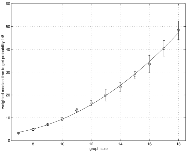
FIG. 1.: Median times to get success probability $1\over 8$ for random graphs with unique maximal cliques. Error bars show the 95% confidence level on the median.

FIG. 2.: Distributions of the run times to get probability $1\over 8$ for 2000 random graphs of size $n=15$ with unique maximal cliques of sizes $k=5$ or $k=6$. Note that the most outlying points are near $T=270$ for $k=5$ and $T=140$ for $k=6$.

To specify a general algorithm for finding cliques in graphs of arbitrary size, we must provide a procedure for choosing the run time $T$ at any value of $n$. We might imagine a procedure wherein we start at some $n$-independent $T$ and repeatedly increase $T$ in some way if the algorithm fails to find a clique. However, if the median time to achieve some fixed probability is truly asymptotically quadratic, and if the distribution about this median is not too broad, a reasonable procedure is to simply choose a run time by extrapolating the fit shown in Fig. 1.

In view of the latter approach, having determined the median run times for $n=15$, we would like to know the distribution of success probabilities at these run times. These distributions are shown in Fig. 3 for $k=5$ and $k=6$, again with 1000 instances at each $k$ and constraining the graphs to have unique maximal cliques. Unsurprisingly, we find median success probabilities near $1\over 8$: $p_{5}=0.120$ and $p_{6}=0.128$. More importantly, the distribution of success probabilities appears to be cut off fairly sharply on the low probability side. Indeed, we find minimum probabilities $p_{5}^{\rm min}=0.031$ and $p_{6}^{\rm min}=0.023$.

FIG. 3.: Distributions of success probabilities at the median run time for 2000 random graphs of size $n=15$ with unique maximal cliques of sizes $k=5$ or $k=6$.

Ultimately, we are interested in the distribution of success probabilities over all random graphs, with or without a unique maximal clique. Fig. 4 shows the distribution of success probabilities without the constraint that the maximal clique is unique, based on 2000 instances at each of $k=5$ and $k=6$. These distributions are shifted towards higher probabilities than in the unique case, with median probabilities $p_{5}^{\prime}=0.232$ and $p_{6}^{\prime}=0.155$, both higher than $1\over 8$. The distributions still fall off sharply on the low probability side. Thus, it is clear that finding non-unique maximal cliques is easier for the quantum algorithm than finding unique ones, and we are justified in having determined the run time using graphs for which the maximal clique is unique.

FIG. 4.: Distribution of success probabilities at the median run time for 4000 random graphs of size $n=15$ with (not necessarily unique) maximal cliques of sizes $k=5$ or $k=6$.

VII Conclusion

We have presented data showing that quantum computation by adiabatic evolution is a reasonable candidate for a fast algorithm to find the largest clique in a random graph. Together with previous studies of the performance of similar methods for solving satisfiability problems, these results suggest that quantum computation by adiabatic evolution may be a useful, general way to attack difficult combinatorial search problems.

REFERENCES

- [1] E. Farhi, J. Goldstone, S. Gutmann, and M. Sipser, Quantum computation by adiabatic evolution, quant-ph/0001106.
- [2] For a related technique, see T. Kadowaki and H. Nishimori, Quantum annealing and the transverse Ising model, cond-mat/9804280; Phys. Rev. E 58, 5355 (1998).
- [3] E. Farhi, J. Goldstone, and S. Gutmann, A numerical study of the performance of a quantum adiabatic evolution algorithm for satisfiability, quant-ph/0007071.
- [4] E. Farhi, J. Goldstone, S. Gutmann, J. Lapan, A. Lundgren, and D. Preda, A quantum adiabatic evolution algorithm applied to an NP-complete problem, to appear.
- [5] A. Messiah, Quantum Mechanics, Vol. II (Wiley, New York, 1976).
- [6] P. Erdös and A. Réyni, On the evolution of random graphs, Publ. Math. Inst. Hung. Acad. Sci. 8, 455 (1964).
- [7] B. Bollobás, Random Graphs (Academic, New York, 1985).
- [8] A. Frieze and C. McDiarmid, Algorithmic theory of random graphs, Random Struct. Alg. 10, 5 (1997).
- [9] D. W. Matula, The employee party problem, Notices Amer. Math. Soc. 19, A-382 (1972).
- [10] M. Jerrum, Large cliques elude the Metropolis process, Random Struct. Alg. 3, 347 (1992).
- [11] A. Juels and M. Peinado, Hiding cliques for cryptographic security, Proc. 9th Annual ACM-SIAM SODA, 678 (1998).
- [12] I. L. Chuang and D. S. Modha, Reversible arithmetic coding for quantum data compression, IEEE Trans. Inf. Theory 46, 1104 (2000).