Decay of an excited atom near an absorbing microsphere

Abstract

Spontaneous decay of an excited atom near a dispersing and absorbing microsphere of given complex permittivity that satisfies the Kramers-Kronig relations is studied, with special emphasis on a Drude-Lorentz permittivity. Both the whispering gallery field resonances below the band gap (for a dielectric sphere) and the surface-guided field resonances inside the gap (for a dielectric or a metallic sphere) are considered. Since the decay rate mimics the spectral density of the sphere-assisted ground-state fluctuation of the radiation field, the strengths and widths of the field resonances essentially determine the feasible enhancement of spontaneous decay. In particular, strong enhancement can be observed for transition frequencies within the interval in which the surface-guided field resonances strongly overlap. When material absorption becomes significant, then the highly structured emission pattern that can be observed when radiative losses dominate reduces to that of a strongly absorbing mirror. Accordingly, nonradiative decay becomes dominant. In particular, if the distance between the atom and the surface of the microsphere is small enough, the decay becomes purely nonradiative.

I Introduction

Light propagating in dielectric spheres can be trapped by repeated total internal reflections. When the round-trip optical paths fit integer numbers of the wavelength, whispering gallery (WG) waves are formed, which combine extreme photonic confinement with very high quality factors. The frequencies and linewidths of WG waves are highly sensitive to strain, temperature, and other parameters of the surrounding environment in general. The unique properties of WG waves are crucial to cavity-QED and various optoelectronics applications [2]. WG waves with $Q$-values larger than $10^{9}$ have been reported for fused-silica microspheres [3, 4, 5] and liquid hydrogen droplets [6], and the ultimate level determined by intrinsic material absorption has been achieved [4].

Since the spontaneous decay of an excited atom depends on both the atom and the ambient medium [7], it can be expected that if an atom is near a dielectric microsphere, its spontaneous decay sensitively responds to the sphere-assisted electromagnetic field structure. In the case of an atom in free space, the well-known continuum of free-space density of modes of radiation is available for an emitted photon. By redistributing the density of possible field excitations in the presence of dielectric bodies, the radiative properties of excited atoms can be controlled. Experimental observations of lifetime modifications of ions or dye molecules embedded in microspheres or droplets [8], cavity QED effects in the coupling of a dilute cesium vapor to the external evanescent field of a WG mode in a fused silica microsphere [9], and detection of individual spatially constrained and oriented molecules on the surfaces of glycerol microdroplets [10] have been reported. In Refs. [11, 12], the decay rate of a two-level atom located in the vicinity of a dielectric sphere was calculated and enhancement factors of hundreds were predicted. The calculations are based on the assumption that there is no material absorption. In practice however, there exists always some material absorption that, even when it is small, can still affect the system in a substantial way. Knowledge of both the radiative losses and the losses due to material absorption is crucial, e.g., in designing ultralow threshold microsphere lasers using cooled atoms or single quantum dots [13].

In the present paper we study the problem of spontaneous decay of an excited atom near an absorbing microsphere of given complex permittivity that satisfies the Kramers-Kronig relations, applying the formalism developed in Refs. [14, 15]. This enables us to take into account both dispersion and absorption in a consistent way, avoiding any restrictive conditions with respect to the frequency domain. In the numerical calculations we assume that the permittivity of the microsphere depends on the frequency according to the Drude-Lorentz model, which covers dielectric and metallic matter.

The paper is organized as follows. In Sec. II the radiation field resonances associated with a microsphere are examined. Equations for determining the positions and widths of both the WG field resonances below a band gap and the surface-guided (SG) field resonances inside a band gap are given. The corresponding quality factors are calculated and the effects of dispersion, absorption, and cavity size are studied. Further, the spatial distribution of the cavity-assisted ground-state fluctuation of the radiation field is studied. In particular, the wings outside the microsphere of the fluctuation of the WG and SG waves are just responsible for exciting such waves in the spontaneous decay of an excited atom that is situated near the surface of the sphere.

In Sec. III the rate of spontaneous decay, the line shift, and the (spatially resolved) intensity of the emitted light are calculated as functions of the atomic transition

FIG. 1.: Real and imaginary parts of the permittivity of a Drude-Lorentz-type dielectric, Eq. (1), for $\omega_{P}$ $\!=$ $\!0.5\,\omega_{T}$ and $\gamma$ $\!=$ $\!10^{-4}\omega_{T}$. The band gap covers the interval from $\omega_{T}$ to $\omega_{L}$ $\!\simeq$ $\!1.12\,\omega_{T}$.

frequency, with special emphasis on the influence of the orientation of the transition dipole moment, the distance between the atom and the microsphere, and the dispersion and absorption outside and inside a band gap. In this context, the ratio of radiative decay to nonradiative decay due to material absorption is analyzed.

In Sec. IV the results derived for the general case of dielectric sphere are applied to a metallic microsphere by appropriately specifying the matter parameters. Typical features are briefly discussed. Finally, some concluding remarks are given in Sec. V.

II Radiation field resonances

Let us consider a dielectric sphere of radius $R$ whose complex permittivity $\epsilon(\omega)$ $\!=$ $\!\epsilon_{R}(\omega)$ $\!+$ $\!i\epsilon_{I}(\omega)$ reads, according to a single-resonance Drude-Lorentz model,

$$\epsilon(\omega)=1+{\omega_{P}^{2}\over\omega_{T}^{2}-\omega^{2}-i\omega\gamma}\,,$$ (1)

where $\omega_{P}$ corresponds to the coupling constant, and $\omega_{T}$ and $\gamma$ are respectively the medium oscillation frequency and the linewidth. An example of the dependence on frequency of the permittivity is shown in Fig. 1. Note that $\epsilon(\omega)$ satisfies the Kramers-Kronig relations. From the permittivity, the complex refractive index can be obtained according to the relations

$$n(\omega)=\sqrt{\epsilon(\omega)}=n_{R}(\omega)+in_{I}(\omega),$$ (2)

$$\displaystyle n_{R(I)}(\omega)=\sqrt{{1\over 2}\left[\sqrt{\epsilon_{R}^{2}(\omega)+\epsilon_{I}^{2}(\omega)}+(-)\,\epsilon_{R}(\omega)\right]}\ .$$ (3)

The dielectric features a band gap between the transverse frequency $\omega_{T}$ and the longitudinal frequency $\omega_{L}$ $\!=$ $\!\sqrt{\omega_{T}^{2}+\omega_{P}^{2}}$. Far from the medium resonances, we typically observe that

$$\epsilon_{I}(\omega)\ll|\epsilon_{R}(\omega)|.$$ (4)

For $\omega$ $\!<$ $\!\omega_{T}$, i.e., outside the band gap, we have

$$\epsilon_{R}(\omega)>1,$$ (5)

$$\displaystyle n_{R}(\omega)\simeq\sqrt{\epsilon_{R}(\omega)}\gg n_{I}(\omega)\simeq{\epsilon_{I}(\omega)\over 2\sqrt{\epsilon_{R}(\omega)}}\,,$$ (6)

and for $\omega_{T}$ $\!<$ $\!\omega$ $\!<\omega_{L}$, i.e., inside the band gap,

$$\epsilon_{R}(\omega)<0,$$ (7)

$$\displaystyle n_{R}(\omega)\simeq{\epsilon_{I}(\omega)\over 2\sqrt{|\epsilon_{R}(\omega)|}}\ll n_{I}(\omega)\simeq\sqrt{|\epsilon_{R}(\omega)|}\,.$$ (8)

Note that $\epsilon_{I}(\omega)$ $\!>$ $\!0$ in any case.

Using the source-quantity representation of the quantized electromagnetic field [15, 16], all the information about the influence of the sphere on the spontaneous decay of an atom is contained in the Green tensor of the classical, phenomenological Maxwell equations, where dispersion and absorption are fully taken into account [14, 15]. In particular, the sphere-assisted (transverse) field resonances that can give rise to an enhancement of the spontaneous decay are determined by the poles of the transverse part of the Green tensor.

From the explicit form of the Green tensor as given in Appendix A, it follows, on setting the denominators in Eqs. (A21) [or (A25)] and (A23) [or (LABEL:A7b)] equal to zero, that the resonances are the complex roots

$$\omega=\Omega-i\delta$$ (9)

of the characteristic equations

$$M(\omega)={H^{\prime}_{l+1/2}(k_{1}R)\over H_{l+1/2}(k_{1}R)}-\sqrt{\epsilon(\omega)}\,{J^{\prime}_{l+1/2}(k_{2}R)\over J_{l+1/2}(k_{2}R)}=0$$ (10)

for TE waves, and

$$M(\omega)={H^{\prime}_{l+1/2}(k_{1}R)\over H_{l+1/2}(k_{1}R)}$$ (12)

$$\hskip 8.61108pt-{1\over\sqrt{\epsilon(\omega)}}{J^{\prime}_{l+1/2}(k_{2}R)\over J_{l+1/2}(k_{2}R)}+{1\over 2k_{1}R}\left[1-{1\over\epsilon(\omega)}\right]=0$$

for TM waves, where $k_{1}$ $\!=$ $\!\omega/c$, $k_{2}$ $\!=$ $\!\sqrt{\epsilon(\omega)}\omega/c$, and $R$ is the microsphere radius [$J_{\nu}(z)$ - Bessel function; $H_{\nu}(z)$ - Hankel function]. In Eq. (9), $\Omega$ and $\delta$, respectively, are the position and the HWHM of a resonance line. Equations (10) and (12) are in agreement with the results of classical Lorenz-Mie scattering theory [2]. Similar equations with real permittivity have also been derived quantum mechanically by expanding the field operators in spherical wave functions [17]. Note that these results cannot be extended to absorbing media by simply replacing the real permittivity by a complex one, but requires a more refined approach to the electromagnetic field quantization in absorbing dielectrics (for details, see [16] and references therein).

The linewidths of the resonances are determined by radiative losses associated with the input-output coupling and losses due to material absorption. For small linewidths, the total width can be regarded as being the sum of a purely radiative term and a purely absorptive term. In that case we may write

$$\delta_{tot}\simeq\delta_{rad}+\delta_{abs},$$ (13)

where $\delta_{rad}$ corresponds to the linewidth obtained when the imaginary part of the permittivity is set equal to zero.

A Resonances below the band gap

We first consider the (transverse) field resonances below the band gap, $\omega$ $\!<$ $\!\omega_{T}$, where WG waves can be observed. These resonances are commonly classified by means of three numbers [2, 3]: the angular momentum number $l$, the azimuthal number $m$, and the number $i$ of radial maxima of the field inside the sphere. In the case of a uniform sphere, the WG waves are ($2l$ $\!+$ $\!1$)-fold degenerate, i.e., the $2l$ $\!+$ $\!1$ azimuthal resonances belong to the same frequency $\Omega_{l,i}$.

When the imaginary part of the refractive index is much smaller than the real part, $n_{I}(\omega)$ $\!\ll$ $\!n_{R}(\omega)$, then the method used in Ref. [18] for solving Eqs. (10) and (12) in the case of constant, real refractive index formally applies also to the case of frequency-dependent, complex refractive index. Interpreting the WG waves as resulting from total internal reflection, it follows that $R{\rm Re}\,k_{2}$ $\gtrsim$ $\!\nu$ $\!\gtrsim$ $\!Rk_{1}$, where $\nu$ $\!=$ $\!l+1/2$, and $\nu$ can be assumed to be large in general. Following Ref. [18], the complex roots $\omega_{l,i}$ of Eqs. (10) and (12) can then formally given by

$$\omega_{l,i}=f_{l,i}[n(\omega_{l,i})]+O(\nu^{-1}),$$ (14)

where

$$f_{l,i}[n(\omega_{l,i})]={c\over Rn(\omega_{l,i})}\Biggl{\{}\nu+2^{-1/3}\alpha_{i}\nu^{1/3}$$ (17)

$$\hskip 8.61108pt-{P\over\left[n(\omega_{l,i})^{2}-1\right]^{1/2}}+{3\over 10}\,2^{-2/3}\alpha_{i}^{2}\nu^{-1/3}$$

$$\hskip 8.61108pt-{2^{-1/3}P\left[n(\omega_{l,i})^{2}-2P^{2}/3\right]\over\left[n(\omega_{l,i})^{2}-1\right]^{3/2}}\,\alpha_{i}\nu^{-2/3}\Biggr{\}},$$

with $P$ $\!=$ $\!n(\omega_{l,i})$ and $P$ $\!=$ $\!1/n(\omega_{l,i})$, respectively, for TE and TM waves, and the $\alpha_{i}$ are the roots of the Airy function Ai$(-z)$. Although Eq. (14) is not yet an explicit expression for the roots as in the case of a nondispersing and nonabsorbing (idealized) medium, it is numerically more tractable than the original equations and offers a first insight into the WG waves.

1 Frequency-independent permittivity

In many cases in practice, it may be a good approximation to ignore the dependence on frequency of the refractive index within a chosen frequency interval. From Eqs. (14) and (17), the positions of the WG waves are then found to be

$$\Omega=f(n_{R})+O\bigg{[}\left(n_{I}\over n_{R}\right)^{2}\bigg{]}\ .$$ (18)

For notational convenience, here and in the following we drop the classification indices. Obviously, the first term in Eq. (18) provides a very good approximation for the positions of the WG waves, provided that the ratio $n_{I}/n_{R}$ is sufficiently small. Note that $n$ $\!\sim$ $\!1.45$ $\!+$ $\!i10^{-11}$ for silica [4] and $n$ $\!\sim$ $\!1.47$ $\!+$ $\!i10^{-7}$ for glycerol [19] in the optical region. In other words, small material absorption does not affect much the positions of the WG waves.

The contribution to the linewidth of the material absorption can be evaluated from Eq. (14) by first order Taylor expansion of $f(n)$ at $n_{R}$,

$$\delta_{abs}\simeq-n_{I}f^{\prime}(n_{R})\ .$$ (19)

To calculate the total line width determined by both radiative and absorption losses, one has to go back to the original equations (10) and (12), since the radiative losses are essentially determined by the (disregarded) term $O(\nu^{-1})$ in Eq. (14). First-order Taylor expansion of $M(\omega)$ around $\Omega$ yields

$$\delta_{tot}\simeq{\rm Im}\left[{M(\Omega)\over M^{\prime}(\Omega)}\right],$$ (20)

where

$$M^{\prime}(\Omega)\simeq\epsilon-1$$ (21)

for TE waves, and

$$M^{\prime}(\Omega)\simeq(\epsilon-1)\left[\left(1+\frac{1}{\epsilon}\right)\left(\frac{c\nu}{R\Omega}\right)^{2}-1\right]$$ (22)

for TM waves. The radiative contribution to the linewidth can then calculated by means of Eq. (13).

From Fig. 2 it is seen that the contribution to the linewidth of the material absorption increase with the imaginary part of the refractive index $n_{I}$ and the radius $R$ of the sphere. It is seen that when the values of $n_{I}$ and $R$ rise above some threshold values, then the absorption losses start to dominate the radiative losses. It is further seen that for chosen $n_{I}$ the threshold value of $R$ decreases with increasing $n_{R}$. For instance, the absorption losses start to dominate the radiative losses if $R$ $\!\gtrsim$ $\!8\lambda$ for $n$ $\!=1.45$ $\!+$ $\!i10^{-9}$ [see Fig. 2(a)], and if $R$ $\!\gtrsim$ $\!1.6\lambda$ for $n$ $\!=$ $\!2.45+i10^{-9}$ [see Fig. 2(b)]. It should be noted, that the approximate results based on Eqs. (19) and (20) are in good agreement with the exact ones (without dispersion).

FIG. 2.: The ratio of the total width $\delta_{tot}$ and the radiative width $\delta_{rad}$ of TM_l,1 WG resonances is shown as a function of the imaginary part $n_{I}$ of the refractive index for two values of the real part $n_{R}$ of the refractive index and various values of $l$. The values $l$ $\!=$ $\!70,\,60,\,50$ correspond to $R/\lambda$ $\!\simeq$ $\!8.4,\,7.3,\,6.2$, respectively, and the values $l$ $\!=$ $\!22,\,20,\,15$ correspond to $R/\lambda$ $\!\simeq$ $\!1.8,\,1.6,\,1.3$, respectively.

Introducing the quality factor $Q$ $\!=$ $\Omega/(2\delta)$, the absorption-assisted part $Q_{abs}$ $\!=$ $\!\Omega/(2\delta_{abs})$ is derived from Eqs. (17)–(19) to be

$$Q_{abs}={n_{R}\over 2n_{I}}+{n_{R}\over 2n_{I}}{(2n_{R}-P)\over(n_{R}^{2}-1)^{3/2}}\,\nu^{-1}+O\bigl{(}\nu^{-5/3}\bigr{)}$$ (23)

[$P$ $\!=$ $\!n_{R}$ $(1/n_{R})$ for TE (TM) waves]. When the absorption losses dominate the radiative ones, it is frequently assumed [4, 20] that the quality factor is simply given by the ratio of the (plane-wave) absorption length and the wavelength, i.e., $Q$ $\!=$ $\!n_{R}/(2n_{I})$, which is just the first term on the right-hand side in Eq. (23). As long as the values of $\nu$ and/or $n_{R}$ are large, which is the case for WG waves, the second term on the right-hand side in Eq. (23) is typically less than a few percent, and the first term is indeed the leading term. Nevertheless, Eq. (23) may become significantly wrong, because dispersion is fully disregarded. Moreover, the radiative losses can dominate material absorption.

2 Frequency-dependent permittivity

In order to obtain the exact quality factor in dependence on the resonance frequency, the permittivity as a function of frequency must be known and the calculations should be based on the original equations (10) and (12). In particular, the quality factor $Q_{rad}$, which accounts for the line broadening associated with the input–output coupling, can be obtained by setting the imaginary part of the permittivity equal to zero, so that $Q$ $\!=$ $\!Q_{rad}$. Recalling Eq. (13), we may write $1/Q$ $\!=$ $1/Q_{tot}$ $\!=$ $\!1/Q_{rad}$ $\!+$ $\!1/Q_{abs}$, from which the quality factor $Q_{abs}$, which accounts for the line broadening due to material absorption, can then be calculated. Typical results obtained for TM WG waves on the basis of the model permittivity in Eq. (1) are shown in Fig. 3.

From Fig. 3(a) it is seen that (for chosen radius of the microsphere) $Q_{abs}$ decreases with increasing frequency (i.e., increasing $n_{I}$ $\!\sim$ $\!\epsilon_{I}$), whereas $Q_{rad}$ increases with increasing frequency (i.e., increasing $n_{R}$ $\!\sim$ $\!\sqrt{\epsilon_{R}}$). Sufficiently below the band gap where $n_{R}$ is small and the radiative losses dominate, $Q_{tot}$ follows $Q_{rad}$. With increasing frequency the absorption losses increase and can eventually dominate the radiative losses, so that now $Q_{tot}$ follows $Q_{abs}$.

In Fig. 3(b), the values of $Q_{abs}$ calculated from the exact equation (12) are compared with the approximate values according to Eq. (23). It is seen that the neglect of dispersion in Eq. (23) leads to some underestimation of the absorption-assisted quality factor. The difference between the exact and the approximate values increase with frequency, because of the increasing dispersion. We have also calculated $Q_{abs}$ from the approximate equation (14) [together with Eq. (17)] and found a good agreement with the exact result.

Figure 3(c) illustrates the influence on the quality factor of the radius of microsphere and the strength of absorption. As expected, for lower frequencies where $Q_{tot}$ follows $Q_{rad}$, the quality is improved if the radius of the sphere is increased. For higher frequencies where $Q_{tot}$ follows $Q_{abs}$, the quality becomes independent of the radius. Note that with increasing radius the (frequency) distance between neighboring resonances decreases.

B Resonances inside the band gap

Let us now look for (transverse) field resonances inside the band gap, which is a strictly forbidden zone for nonabsorbing bulk material. Inside the gap, we may assume that the real part of the refractive index is much smaller than the imaginary part, $n_{R}(\omega)$ $\!\ll$ $\!n_{I}(\omega)$. Using Bessel-function expansion (Appendix B), it can be shown that there are no TE resonances [Eq. (10) has no solutions], and the complex roots of Eq. (12), which determine the TM resonances, can formally be given by

FIG. 3.: Quality factors of TM_l,1 WG field resonances in a dielectric microsphere of radius $R$ and complex permittivity $\epsilon(\omega)$ according to Eq. (1) ($\omega_{P}$ $\!=$ $\!0.5\,\omega_{T}$). (a) Exact values of $Q_{rad}$, $Q_{abs}$, and $Q_{tot}$ for $R$ $\!=$ $\!10\,\lambda_{T}$, $\gamma$ $\!=$ $\!10^{-6}\omega_{T}$, $48$ $\!\leq$ $\!l$ $\!\leq$ $\!78$. (b) Exact values of $Q_{abs}$ (+) and approximate values ($\triangle$) according to Eq. (23) for the same parameters as in (a). (c) Exact values of $Q_{tot}$ for $\gamma/\omega_{T}$ $\!=$ $\!10^{-6}$ ($\circ$) and $\gamma/\omega_{T}$ $\!=$ $\!10^{-4}$ ($\triangle$); (1) $R$ $\!=$ $\!10\,\lambda_{T}$, $48$ $\!\leq$ $\!l$ $\!\leq$ $\!78$; (2) $R$ $\!=$ $\!2\,\lambda_{T}$, $10$ $\!\leq$ $\!l$ $\!\leq$ $\!22$.

$$\omega_{l}={c\over R}\Biggl{[}\nu\sqrt{1\!+\!{1\over\epsilon(\omega_{l})}}+{\epsilon(\omega_{l})^{2}\!+\!\epsilon(\omega_{l})\!+\!1\over 2\epsilon(\omega_{l})\sqrt{-\epsilon(\omega_{l})\!-\!1}}\Biggr{]}+O\bigl{(}\nu^{-1}\bigr{)},$$ (24)

where the condition

FIG. 4.: Quality factors of TM_l SG field resonances in a dielectric microsphere of radius $R$ and complex permittivity $\epsilon(\omega)$ according to Eq. (1) ($\omega_{P}$ $\!=$ $\!0.5\,\omega_{T}$). (a) Exact values of $Q_{rad}$, $Q_{abs}$, and $Q_{tot}$ for $R$ $\!=$ $\!10\,\lambda_{T}$, $\gamma$ $\!=$ $\!10^{-6}\omega_{T}$, $70$ $\!\leq$ $\!l$ $\!\leq$ $\!120$. (b) Exact values of $Q_{abs}$ (+) and approximate values ($\triangle$) according to Eq. (27) for the same parameters as in (a). (c) Exact values of $Q_{tot}$ for $\gamma/\omega_{T}$ $\!=$ $\!10^{-6}$ ($\circ$) and $\gamma/\omega_{T}$ $\!=$ $\!10^{-4}$ ($\triangle$); (1) $R$ $\!=$ $\!10\lambda_{T}$, $70$ $\!\leq$ $\!l$ $\!\leq$ $\!86$; (2) $R$ $\!=$ $\!2\,\lambda_{T}$, $15$ $\!\leq$ $\!l$ $\!\leq$ $\!55$. The gap is from $\omega_{T}$ to $\omega_{L}\simeq 1.12\,\omega_{T}$ [cf. Fig.1]. According to Eq. (26), resonances exist for $\Omega_{l}$ $\!<$ $\!1.0607\,\omega_{T}$.

$$\epsilon_{R}(\omega_{l})<-1$$ (25)

has been required to be satisfied. Note that for the Drude-Lorentz model (1), condition (25) leads to

$$\Omega_{l}={\rm Re}\,\omega_{l}<\sqrt{\omega_{T}^{2}+{\textstyle\frac{1}{2}}\omega_{P}^{2}}\,.$$ (26)

The total linewidth can be determined according to Eq. (20), which is still valid here. If we ignore the dependence on frequency of the permittivity, then the expression on the right-hand side of Eq. (24) can be regarded as a function of the refractive index. The contribution to the linewidth of the material absorption can then be calculated by first-order Taylor expansion at $n_{I}$ of this function in close analogy to Eq. (19) (with the roles of $n_{R}$ and $n_{I}$ being exchanged). In terms of the quality factor $Q_{abs}$ $\!=$ $\!\Omega/(2\delta_{abs})$ the result reads

$$Q_{abs}=\frac{n_{I}(n_{I}^{2}\!-\!1)}{2n_{R}}+O\bigl{(}\nu^{-1}\bigr{)}.$$ (27)

Since now $n_{R}$ is proportional to $\gamma$, $Q_{abs}$ is again proportional to $\gamma^{-1}$.

It is well known that when the condition (25) is satisfied, then surface-guided (SG) waves can be excited – waves that are bound to the interface and whose amplitudes are damped into either of the neighboring media [21]. Typical examples are surface phonon polaritons for dielectrics and surface plasmon polaritons for metals. Obviously, the TM resonances as determined by Eq. (24) correspond to SG waves of a sphere. Note that for the SG waves, in contrast to the WG waves, each angular momentum number $l$ is associated with only one wave.

Examples of the frequencies and quality factors of SG waves are plotted in Fig. 4. From a comparison with Fig. 3 it is seen that the quality factors of the SG waves are comparable with those of the WG waves and also behave in a similar way as the latter. So, the radiative losses are the dominant ones for lower-order resonances, whereas for higher-order resonances the losses essentially arise from material absorption [Figs. 4(a) and (c)], and the radiative losses can be reduced by increasing the radius of the sphere [Fig. 4(c)]. Further, a neglect of dispersion again leads to some overestimation of material absorption [Fig. 4(b)].

C Ground-state fluctuations

When an excited atom is in free space, then its coupling to the vacuum-field fluctuation gives rise to spontaneous decay. In the presence of dielectric bodies, the fluctuation of the electromagnetic field with respect to the ground-state of the combined system that consists of the radiation field and the dielectric matter must be considered. The electric-field correlation in the ground state can be characterized by the correlation function

FIG. 5.: Spatial variation of the ground-state fluctuations $P_{rr}({\bf r},\omega)$ (in arbitrary units) inside a dielectric microsphere of radius $R$ $\!=$ $\!2\,\lambda_{T}$ and complex permittivity $\epsilon(\omega)$ according to Eq. (1) [$\omega_{P}$ $\!=$ $\!0.5\,\omega_{T}$; $\gamma/\omega_{T}$ $\!=$ $\!10^{-4}$ (solid line), $10^{-6}$ (dashed line), and $10^{-8}$ (dotted line)]. (a) $\omega$ $\!=$ $\!0.94042\,\omega_{T}$, TM_16,1 WG field resonance. (b) $\omega$ $\!=$ $\!1.02811\,\omega_{T}$, TM₁₆ SG field resonance. (c) $\omega$ $\!=$ $\!1.05339\,\omega_{T}$, TM₃₀ SG field resonance.

$$\langle 0|\underline{\hat{E}}_{i}({\bf r},\omega)\underline{\hat{E}}^{\dagger}_{j}({\bf r}^{\prime},\omega^{\prime})|0\rangle$$ (29)

$$\hskip 8.61108pt={\hbar\omega^{2}\over\pi\epsilon_{0}c^{2}}{\rm Im}\ G_{ij}({\bf r},{\bf r}^{\prime},\omega)\delta(\omega-\omega^{\prime})\ ,$$

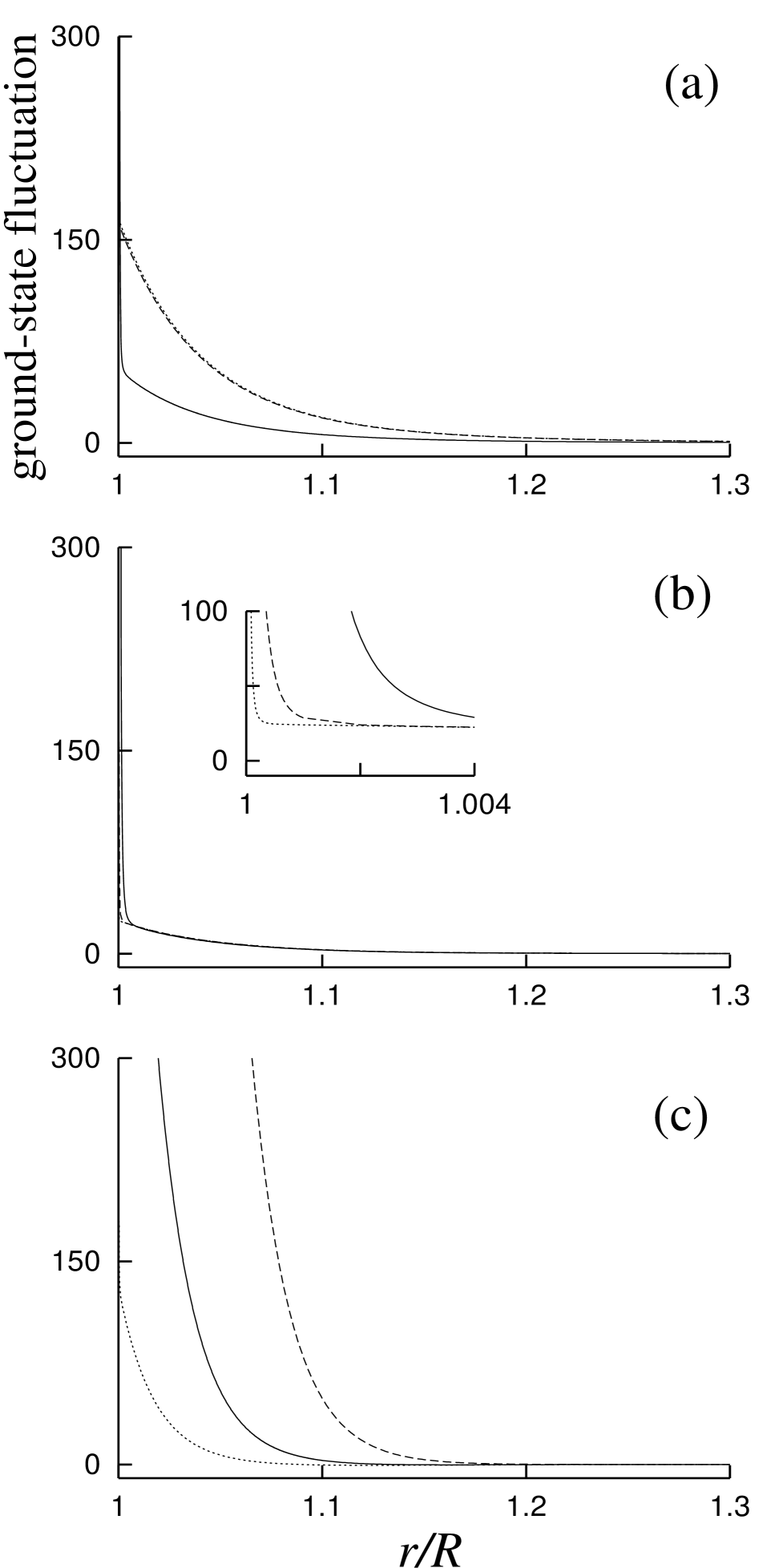
FIG. 6.: The same as in Fig. 5, but for outside the sphere.

where $\underline{\hat{E}}_{i}({\bf r},\omega)$ is the electric-field operator in the frequency domain and $G_{ij}({\bf r},{\bf r}^{\prime},\omega)$ is the classical Green tensor of the dielectric-matter formation of given complex permittivity $\epsilon({\bf r},\omega)$ that satisfies the Kramers-Kronig relations. For equal spatial arguments, the power spectrum of the ground-state fluctuation can be obtained according to the relation

$$\langle 0|\underline{\hat{E}}_{i}({\bf r},\omega)\underline{\hat{E}}^{\dagger}_{j}({\bf r},\omega^{\prime})|0\rangle=P_{ij}({\bf r},\omega)\delta(\omega-\omega^{\prime}),$$ (30)

which together with Eq. (29) reveals that

$$P_{ij}({\bf r},\omega)={\hbar\omega^{2}\over\pi\epsilon_{0}c^{2}}\,{\rm Im}\ G_{ij}({\bf r},{\bf r},\omega).$$ (31)

From the linearity of the Maxwell equations it follows that the Green tensor for a dielectric body can be decomposed as [cf. Eq. (A1)]

$$G_{ij}({\bf r},{\bf r}^{\prime},\omega)=G_{ij}^{0}({\bf r},{\bf r}^{\prime},\omega)+G_{ij}^{R}({\bf r},{\bf r}^{\prime},\omega),$$ (32)

where $G_{ij}^{0}$ is the Green tensor for either the vacuum (outside the body) or the bulk material (inside the body), and the scattering term $G_{ij}^{R}$ ensures the correct boundary conditions (at the surface of discontinuity). Inside the body ${\rm Im}\,G_{ij}^{0}$ becomes singular for ${\bf r}$ $\!\to$ $\!{\bf r}^{\prime}$, and some regularization (e.g., averaging over a small volume) is required. Since we are only interested in the spatial variation of the ground-state fluctuation, we may disregard the (space-independent) contribution that arises from ${\rm Im}\,G_{ij}^{0}$.

The spatial variation of the radial diagonal component $P_{rr}$ inside and outside the microsphere under consideration is illustrated in Figs. 5 and 6, respectively. Note that $P_{rr}$ only refers to the TM field noise [cf. Eqs. (A9) – (A19)]. It is seen that the fluctuation associated with the WG-type field [Figs. 5(a) and 6(a)] essentially concentrates inside the sphere, whereas the fluctuation associated with the SG-type field [Figs. 5(b,c) and 6(b,c)] concentrates in the vicinity of the surface of the sphere. In both cases, a singularity is observed at the surface. In Figs. 5(a) and 6(a), we have restricted our attention to a single-maximum WG field, i.e., $i$ $\!=$ $\!1$. Otherwise $i$ ($>$ $\!1$) maxima would be observed inside the sphere.

The strong enhancement of the fluctuation which leads to the singularity at the surface comes from absorption and gives rise to nonradiative energy transfer from the atom to the medium (see Sec. III B). Clearly, for sufficiently small absorption the divergence becomes meaningless, because the required (small) spatial resolution would be illicit. From Figs. 5(a) and 6(a) it is seen that material absorption reduces the fluctuation of the WG field inside and outside the sphere, and Figs. 5(b,c) and 6(b,c) show that absorption changes the area on either side of the surface over which the SG field fluctuation extends. As expected, the effects are less pronounced for low-order resonances where the radiative losses are the dominant ones [compare Figs. 5(b) and (c) with Figs. 6(b) and (c) respectively].

III Spontaneous decay

A Basic formulae

In the weak-coupling regime, an excited atom near a a dispersing and absorbing body decays exponentially, where the decay rate is given by

$$A={2k_{A}^{2}\mu_{i}\mu_{j}\over\hbar\epsilon_{0}}\,{\rm Im}\,G_{ij}({\bf r}_{A},{\bf r}_{A},\omega_{A}),$$ (33)

($k_{A}$ $\!=$ $\!\omega_{A}/c$; $\textstyle\mu$, atomic transition dipole moment), and the contribution of the body to the shift of the transition frequency reads

$$\delta\omega_{A}={\mu_{i}\mu_{j}\over\pi\hbar\epsilon_{0}}\,{\cal P}\!\int_{0}^{\infty}d\omega\,{\omega^{2}\over c^{2}}\frac{{\rm Im}\,G_{ij}^{R}({\bf r}_{A},{\bf r}_{A},\omega)}{\omega-\omega_{A}}\,,$$ (34)

which can be rewritten, on using the Kramers-Kronig relations, as

$$\delta\omega_{A}={k_{A}^{2}\mu_{i}\mu_{j}\over\hbar\epsilon_{0}}\,\biggl{[}{\rm Re}\,G_{ij}^{R}({\bf r}_{A},{\bf r}_{A},\omega_{A})$$ (36)

$$\hskip 8.61108pt-\,{{\cal P}\over\pi}\!\int_{0}^{\infty}d\omega\,{\omega^{2}\over\omega_{A}^{2}}\frac{{\rm Im}\,G_{ij}^{R}({\bf r}_{A},{\bf r}_{A},\omega)}{\omega+\omega_{A}}\biggr{]}$$

(for details, see [14, 15]). It is not difficult to see that in Eq. (36) the second term, which is not sensitive to the atomic transition frequency, is small compared to the first one and can therefore be neglected. Note that the vacuum Lamb shift (see, e.g., [22]) may be thought of as being already included in the atomic transition frequency.

The intensity of the spontaneously emitted light registered by a pointlike photodetector at position ${\bf r}$ and time $t$ reads [14]

$$I({\bf r},t)=\sum_{i}\biggl{|}{k_{A}^{2}\mu_{j}\over\pi\epsilon_{0}}\int_{0}^{t}dt^{\prime}\Big{[}C_{u}(t^{\prime})$$ (38)

$$\hskip 8.61108pt\times\int_{0}^{\infty}d\omega\,{\rm Im}\,G_{ij}({\bf r},{\bf r}_{A},\omega)e^{-i(\omega-\omega_{A})(t-t^{\prime})}\Big{]}\biggr{|}^{2},$$

where $C_{u}(t)$ is the probability amplitude of finding the atom in the upper state. Note that Eq. (38) is valid for an arbitrary coupling regime. In particular, in the weak coupling regime, where the Markov approximation applies, $C_{u}(t^{\prime})$ can be taken at $t^{\prime}$ $\!=$ $\!t$ and put in front of the time integral in Eq. (38), with $C_{u}(t)$ being simply the exponential

$$C_{u}(t)=e^{\left(-A/2+i\delta\omega_{A}\right)t}\ .$$ (39)

Equation (38) thus simplifies to

$$I({\bf r},t)\simeq|{\bf F}({\bf r},{\bf r}_{A},\omega_{A})|^{2}e^{-At},$$ (40)

where

$$F_{i}({\bf r},{\bf r}_{A},\omega_{A})=-{ik_{A}^{2}\mu_{j}\over\epsilon_{0}}\biggl{[}G_{ij}({\bf r},{\bf r}_{A},\omega_{A})$$ (42)

$$\hskip 8.61108pt-\,{{\cal P}\over\pi}\int_{0}^{\infty}d\omega\,\frac{{\rm Im}\,G_{ij}({\bf r},{\bf r}_{A},\omega)}{\omega+\omega_{A}}\biggr{]}.$$

Since the second term on the right-hand side of Eq. (42) is small compared to the first one, it can be omitted, and the spatial distribution of the emitted light (emission pattern) can be given by, on disregarding transit time delay,

$$|{\bf F}({\bf r},{\bf r}_{A},\omega_{A})|^{2}\simeq\sum_{i}\biggl{|}{k_{A}^{2}\mu_{j}\over\epsilon_{0}}G_{ij}({\bf r},{\bf r}_{A},\omega_{A})\biggr{|}^{2}.$$ (43)

Material absorption gives rise to nonradiative decay. Obviously, the rate (33) as the total decay rate describes both radiative decay and nonradiative decay. The fraction of emitted radiation energy can be obtained by integration of $I({\bf r},t)$ with respect to time and integration over the surface of a sphere whose radius is much larger than the extension of the system,

$$W=2c\epsilon_{0}\int_{0}^{\infty}dt\int_{0}^{2\pi}d\phi\int_{0}^{\pi}d\theta\,\rho^{2}\sin\theta\,I({\bf r},t)$$ (44)

($\textstyle\rho$ $\!=$ $\!{\bf r}$ $\!-$ $\!{\bf r}_{A}$). The ratio $W/W_{0}$, where $W_{0}$ $\!=$ $\!\hbar\omega_{A}$ is the emitted energy in free space, then gives us a measure of the emitted energy, and accordingly, $1$ $\!-$ $\!W/W_{0}$ measures the energy absorbed by the body.

B Spontaneous decay rate

Using Eqs. (A1) – (A9) and (A14) – (A19), the decay rate (33) for a (with respect to the microsphere) radially oriented transition dipole moment can be given by

$$A^{\perp}=A_{0}\biggl{\{}1+{\textstyle{3\over 2}}\sum_{l=1}^{\infty}l(l+1)(2l+1)$$ (46)

$$\hskip 8.61108pt\times\;{\rm Re}\,\biggl{[}{\cal B}^{N}_{l}\!(\omega_{A})\biggl{(}{h^{(1)}_{l}({k_{A}r_{A}})\over{k_{A}r_{A}}}\biggr{)}^{2}\biggr{]}\biggr{\}},$$

and for a tangential dipole it reads

$$A^{\parallel}=A_{0}\biggl{\{}1+{\textstyle{3\over 4}}\sum_{l=1}^{\infty}(2l+1)$$ (49)

$$\hskip 8.61108pt\times\;{\rm Re}\,\biggl{[}{\cal B}^{M}_{l}\!(\omega_{A})\left(h^{(1)}_{l}({k_{A}r_{A}})\right)^{2}$$

$$\hskip 8.61108pt+\,{\cal B}^{N}_{l}\!(\omega_{A})\biggl{(}{\bigl{[}{k_{A}r_{A}}h^{(1)}_{l}({k_{A}r_{A}})\bigr{]}^{\prime}\over{k_{A}r_{A}}}\biggr{)}^{2}\biggr{]}\biggr{\}},$$

where the prime indicates the derivative with respect to $k_{A}r_{A}$, and

$$A_{0}={k_{A}^{3}\mu^{2}\over 3\hbar\pi\epsilon_{0}}$$ (50)

is the rate of spontaneous emission in free space. Note that a radially oriented transition dipole moment only couples to TM waves, whereas a tangentially oriented dipole moment couples to both TM and TE waves. Equations (46) and (49) generalize the results obtained for nondispersing and nonabsorbing matter whose resonance frequencies are far from the atomic transition frequencies, i.e., $\epsilon$ $\!=$ $\epsilon_{R}$ $\!>$ $\!1$, [11, 12] to arbitrary Kramers-Kronig consistent matter, without placing restrictions to the transition frequency.

FIG. 7.: Decay rate versus atomic transition frequency for a radially oscillating dipole near a microsphere of radius $R$ $\!=$ $\!2\,\lambda_{T}$ and complex permittivity $\epsilon(\omega)$ according to Eq. (1) ($\omega_{P}$ $\!=$ $\!0.5\,\omega_{T}$, $\gamma/\omega_{T}$ $\!=$ $\!10^{-4}$). (a) $\Delta r$ $\!=$ $\!0.02\,\lambda_{T}$; inset: $\gamma/\omega_{T}$ $\!=$ $\!\!10^{-4}$ (solid line), $10^{-5}$ (dashed line), $10^{-6}$ (dotted line). (b) $\Delta r$ $\!=$ $\!0.1\,\lambda_{T}$.

When the atom is very close to the microsphere, Eqs. (46) and (49) simplify to (see Appendix C)

$$A^{\perp}={3A_{0}\over 4k_{A}^{3}}{\epsilon_{I}(\omega_{A})\over|\epsilon(\omega_{A})+1|^{2}}{1\over(\Delta r)^{3}}+O(1)$$ (51)

and

$$A^{\parallel}={3A_{0}\over 8k_{A}^{3}}{\epsilon_{I}(\omega_{A})\over|\epsilon(\omega_{A})+1|^{2}}\left[{1\over(\Delta r)^{3}}+{1\over 2R^{2}\Delta r}\right]+O(1),$$ (52)

with $\Delta r$ $\!=$ $\!r_{A}$ $\!-$ $\!R$ being the distance between the atom and the surface of the microsphere. The terms $\sim$ $\!(\Delta r)^{-3}$ and $\sim$ $\!(\Delta r)^{-1}$ result from the TM near-field coupling. Since they are proportional to $\epsilon_{I}$, they describe nonradiative decay, i.e., energy transfer from the atom to the medium, and reflect the strong enhancement of the electromagnetic-field fluctuation as $\Delta r$ $\!\to$ $\!0$ (see Sec. II C). In particular, the terms $\sim$ $\!(\Delta r)^{-3}$ in Eqs. (51) and (52) are exactly the same as in the case when the atom is close to a planar interface [23, 24]. Obviously, nonradiative decay does not respond sensitively to the actual radiation-field structure. Since the distance of the atom from the surface of the microsphere must not be smaller than interatomic distances (otherwise the concept of macroscopic electrodynamics fails), the divergence at the surface ($\Delta r$ $\!=$ $\!0$) is not observed.

The dependence of the decay rate (46) on the radiation-field structure, which can be observed for not too small (large) values of $\Delta r$ ($\epsilon_{I}$), is illustrated in Fig. 7 for a radially oriented transition dipole moment. Since the decay rate is proportional to the spectral density of final states, its dependence on the transition frequency mimics the excitation spectrum of the sphere-assisted radiation field. As a result, both the WG and SG field resonances can strongly enhance the spontaneous decay. The enhancement decreases with increasing distance between the atom and the sphere [compare Figs. 7(a) an(b)]. When material absorption increases, then the resonance lines are broadened at the expense of the heights and the enhancement is accordingly reduced [see the inset in Fig. 7(a)].

Figure 7 reveals that the SG field resonances, which are the more intense ones in general, can give rise to a much stronger enhancement of the spontaneous decay than the WG field resonances. In particular, with increasing angular-momentum number the lines of the SG field resonances strongly overlap and huge enhancement factors can be observed for transition frequencies inside the band gap [e.g., factors of the order of magnitude of $10^{4}$ for the parameters chosen in Fig. 7(a)]. When the distance between the atom and the sphere increases, then the atom rapidly decouples from that part of the field. Thus, the huge enhancement of spontaneous decay rapidly reduces and the interval in which inhibition of spontaneous decay is typically observed, extends accordingly [see Fig. 7(b)].

C Lamb shift

Substituting expressions (A9) and (A14) – (A19) into Eq. (36), we find that the shift of the atomic transition frequency, which is caused by the presence of the microsphere, is

$$\delta\omega_{A}^{\perp}=-{3A_{0}\over 4}\sum_{l=1}^{\infty}l(l+1)(2l+1)$$ (54)

$$\hskip 8.61108pt\times\;{\rm Im}\biggl{\{}{\cal B}^{N}_{l}\!(\omega_{A})\biggl{[}{h^{(1)}_{l}({k_{A}r_{A}})\over{k_{A}r_{A}}}\biggr{]}^{2}\biggr{\}}$$

for a radially oriented transition dipole moment, and

$$\delta\omega_{A}^{\parallel}=-{3A_{0}\over 8}\sum_{l=1}^{\infty}(2l+1)$$ (57)

$$\hskip 8.61108pt\times\;{\rm Im}\biggl{\{}{\cal B}^{M}_{l}\!(\omega_{A})\left[h^{(1)}_{l}({k_{A}r_{A}})\right]^{2}$$

$$\hskip 8.61108pt+\,{\cal B}^{N}_{l}\!(\omega_{A})\biggl{[}{\bigl{[}{k_{A}r_{A}}h^{(1)}_{l}({k_{A}r_{A}})\bigr{]}^{\prime}\over{k_{A}r_{A}}}\biggr{]}^{2}\biggr{\}}$$

for a tangentially oscillating dipole. In particular, when the distance between the atom and the sphere is very small, then Eqs. (54) and (57) simplify to [in close analogy to Eqs. (51) and (52)]

$$\delta\omega_{A}^{\perp}=-{3A_{0}\over 16k_{A}^{3}}{|\epsilon(\omega_{A})|^{2}-1\over|\epsilon(\omega_{A})+1|^{2}}{1\over(\Delta r)^{3}}+O(1)$$ (58)

and

$$\delta\omega_{A}^{\parallel}=-{3A_{0}\over 32k_{A}^{3}}{|\epsilon(\omega_{A})|^{2}\!-\!1\over|\epsilon(\omega_{A})\!+\!1|^{2}}\left[{1\over(\Delta r)^{3}}+{1\over 2R^{2}\Delta r}\right]+O(1).$$ (59)

The terms $\sim$ $\!(\Delta r)^{-3}$ and $\sim$ $\!(\Delta r)^{-1}$ again result from the TM near-field coupling, and the leading terms agree with those obtained for a planar interface [24]. Note that in contrast to the decay rate, the Lamb shift diverges for $\Delta r$ $\!\to$ $\!0$ even when $\epsilon_{I}$ $\!=$ $\!0$.

The dependence of the frequency shift (54) on the radiation-field structure for not too small values of $\Delta r$ is illustrated in Fig. 8. It is seen that each field resonance can give rise to a noticeable frequency shift in the very vicinity of the resonance frequency; transition frequencies that are lower (higher) than the resonance frequency are shifted to lower (higher) frequencies. In close analogy to the behavior of the decay rate, the shift is more pronounced for SG field resonances than for WG field resonances and can be huge for large angular momentum numbers when the lines of the SG field resonances strongly overlap.

The behavior of the Lamb shift as shown in Fig. 8(b) can already be seen in the single-resonance limit [25]. If the atomic transition frequency $\omega_{A}$ is close to a resonance frequency $\Omega$ of the microsphere, contribution from other resonances may be ignored in a first approximation. Regarding the resonance line as being a Lorentzian and using contour integration, we obtain from Eq. (34)

$$\delta\omega_{A} \simeq -{A(\Omega)\delta^{2}\over 4\pi}\,{\cal P}\!\!\int_{-\infty}^{\infty}\!\!d\omega\,{1\over\omega\!-\!\omega_{A}}{1\over(\omega\!-\!\Omega)^{2}\!+\!\delta^{2}}$$ (60)

$$= -{A(\Omega)\delta\over 2}{\Delta\over\Delta^{2}+\delta^{2}}\,,$$ (61)

where $A(\Omega)$ is the decay rate as given by Eq. (33) (with $\Omega$ in place of $\omega_{A}$), and $\Delta$ $\!=$ $\!\omega_{A}$ $\!-$ $\!\Omega$. In particular, Eq. (60) indicates that the frequency shift peaks at half maximum on both sides of the resonance line. With increasing material absorption, the linewidth $\delta$ increases while $A(\Omega)$ decreases and thus the absolute values of the frequency shift are reduced, the distance between the maximum and the minimum being somewhat increased. With decreasing distance between the atom and the microsphere near-field effects become important and Eq. (60) fails, as it can be seen from a comparison of Figs. 8(a) and (b).

FIG. 8.: Lamb shift versus atomic transition frequency for a radially oscillating dipole near a microsphere of radius $R$ $\!=$ $\!2\,\lambda_{T}$ and complex permittivity $\epsilon(\omega)$ according to Eq. (1) ($\omega_{P}$ $\!=$ $\!0.5\,\omega_{T}$, $\gamma/\omega_{T}$ $\!=$ $\!10^{-4}$). (a) $\Delta r$ $\!=$ $\!0.02\,\lambda_{T}$. (b) $\Delta r$ $\!=$ $\!0.1\,\lambda_{T}$; inset: $\gamma/\omega_{T}$ $\!=$ $\!\!10^{-4}$ (solid line), $10^{-5}$ (dashed line), $10^{-6}$ (dotted line).

D Emitted-light intensity

1 Spatial distribution

Using Eqs. (A1) – (A19), the function ${\bf F}({\bf r},{\bf r}_{A},\omega_{A})$, Eq. (42), which determines, according to Eq. (40), the spatial distribution of the emitted light, can be given by ($\theta_{A}$ $\!=$ $\!\phi_{A}$ $\!=$ $\!0$, $r_{A}$ $\!\leq$ $\!r$)

$${\bf F}^{\perp}({\bf r},{\bf r}_{A},\omega_{A})={k_{A}^{3}\mu\over 4\pi\epsilon_{0}}\sum_{l=1}^{\infty}(2l+1)$$ (65)

$$\hskip 8.61108pt\times\;{1\over{k_{A}r_{A}}}\left[j_{l}({k_{A}r_{A}})+{\cal B}_{l}^{N}\!(\omega_{A})h_{l}^{(1)}({k_{A}r_{A}})\right]$$

$$\hskip 8.61108pt\times\,\biggl{[}{\bf e}_{r}\,l(l\!+\!1)\,{h_{l}^{(1)}({k_{A}r})\over{k_{A}r}}\,P_{l}(\cos\theta)$$

$$\hskip 17.22217pt-\,{\bf e}_{\theta}\,{[{k_{A}r}\,h_{l}^{(1)}({k_{A}r})]^{\prime}\over{k_{A}r}}\,\sin\theta P_{l}^{\prime}(\cos\theta)\biggr{]}$$

for a radially oriented transition dipole moment, and

$${\bf F}^{\parallel}({\bf r},{\bf r}_{A},\omega_{A})={k_{A}^{3}\mu\over 4\pi\epsilon_{0}}\sum_{l=1}^{\infty}{(2l+1)\over l(l+1)}$$ (71)

$$\times\biggl{\{}{\bf e}_{r}\cos\phi\tilde{\cal B}_{l}^{N}l(l\!+\!1)\,{h_{l}^{(1)}({k_{A}r})\over{k_{A}r}}\,\sin\theta P_{l}^{\prime}(\cos\theta)$$

$$\hskip 8.61108pt+\,{\bf e}_{\theta}\cos\phi\biggl{[}\tilde{\cal B}_{l}^{M}h_{l}^{(1)}({k_{A}r})P_{l}^{\prime}(\cos\theta)$$

$$\hskip 34.44434pt+\,\tilde{\cal B}_{l}^{N}\,{[{k_{A}r}\,h_{l}^{(1)}({k_{A}r})]^{\prime}\over{k_{A}r}}\,\tilde{P}_{l}(\cos\theta)\biggr{]}$$

$$\hskip 8.61108pt-\,{\bf e}_{\phi}\sin\phi\biggl{[}\tilde{\cal B}_{l}^{M}h_{l}^{(1)}({k_{A}r})\tilde{P}_{l}(\cos\theta)$$

$$\hskip 34.44434pt+\,\tilde{\cal B}_{l}^{N}\,{[{k_{A}r}\,h_{l}^{(1)}({k_{A}r})]^{\prime}\over{k_{A}r}}\,P_{l}^{\prime}(\cos\theta)\biggr{]}\biggr{\}}$$

for a tangentially oriented dipole in the $xz$-plane. Here, the abbreviating notations

$$\tilde{\cal B}_{l}^{N}={1\over{k_{A}r_{A}}}\Big{\{}[{k_{A}r_{A}}j_{l}({k_{A}r_{A}})]^{\prime}$$ (73)

$$\hskip 8.61108pt+\,{\cal B}_{l}^{N}\!(\omega_{A})[{k_{A}r_{A}}h_{l}^{(1)}({k_{A}r_{A}})]^{\prime}\Big{\}},$$

$$\tilde{\cal B}_{l}^{M}=j_{l}({k_{A}r_{A}})+{\cal B}_{l}^{M}\!(\omega_{A})h_{l}^{(1)}({k_{A}r_{A}}),$$ (74)

$$\tilde{P}_{l}(\cos\theta)=l(l+1)P_{l}(\cos\theta)-\cos\theta P^{\prime}_{l}(\cos\theta)$$ (75)

have been introduced. Examples of the far-field emission pattern of a radially oriented transition dipole moment, $|{\bf F}^{\perp}({\bf r},{\bf r}_{A},\omega_{A})|^{2}$, and a tangentially oriented transition dipole moment, $|{\bf F}^{\|}({\bf r},{\bf r}_{A},\omega_{A})|^{2}$, are plotted in Figs. 9 and 10 respectively.

Let us first restrict our attention to a radially oriented transition dipole moment. In this case, the far field is essentially determined by $F^{\perp}_{\theta}$, as an inspection of Eq. (65) reveals. When the atomic transition frequency coincides with the frequency of a WG wave of angular momentum number $l$ far from the band gap [Fig. 9(a)], then the corresponding $l$-term in the series (65) obviously yields the leading contribution to the emitted radiation, whose angular distribution is significantly determined by the term $\sim$ $\!\sin\theta\,P^{\prime}_{l}(\cos\theta)$. Since $P_{l}(\cos\theta)$ is a polynomial with $l$ real, single roots in the interval $0$ $\!<$ $\!\theta$ $\!<$ $\!\pi$ [26], $\sin\theta\,P^{\prime}_{l}(\cos\theta)$ must have $l$ extrema within this interval. Thus, the emission pattern has $l$ lobes in, say, the $yz$-plane, i.e., $l$ cone-shaped peaks around the $z$-axis, because of symmetry reasons. The lobes near $\theta$ $\!=$ $\!0$ and $\theta$ $\!=$ $\!\pi$ are the most dominant ones in general, because of [27]

$$-\sin\theta P^{\prime}_{l}(\cos\theta)\sim(\sin\theta)^{-1/2}+O\bigr{(}l^{-1}\bigl{)}$$ (76)

($0$ $\!<$ $\!\theta$ $\!<$ $\!\pi$). Note that the superposition of the leading term with the remaining terms in the series (65) gives rise to some asymmetry with respect to the plane $\theta$ $\!=$ $\!\pi/2$.

FIG. 9.: Polar diagrams of the normalized far-field emission pattern $|{\bf F}^{\perp}({\bf r},{\bf r}_{A},\omega_{A})|^{2}/(k_{A}^{3}\mu/4\pi\epsilon_{0})^{2}$ of a radially oscillating dipole near a microsphere of radius $R$ $\!=$ $\!2\,\lambda_{T}$ and complex permittivity $\epsilon(\omega)$ according to Eq. (1) ($\omega_{P}$ $\!=$ $\!0.5\,\omega_{T}$, $\gamma/\omega_{T}$ $\!=$ $\!10^{-4}$, $\Delta r$ $\!=$ $\!0.02\,\lambda_{T}$, $r$ $\!=$ $\!20\lambda_{T}$). $\omega_{A}/\omega_{T}\!=\!$ (a) 0.94042, (b) 0.999, (c) 1.02811, and (d) 1.06.

FIG. 10.: The same as in Fig. 9, but for a tangentially oscillating dipole.

When the atomic transition frequency approaches the band gap (but is still outside it), a strikingly different behavior is observed [Fig. 9(b)]. The emission pattern changes to a two-lobe structure similar to that observed in free space, but bent away from the microsphere surface, the emission intensity being very small. Since near the band gap absorption losses dominate, a photon that is resonantly emitted is almost certainly absorbed and does not contribute to the far field in general. If the photon is emitted in a lower-order WG wave where radiative losses dominate, it has a bigger chance to escape. The superposition of all these weak (off-resonant) contributions just form the two-lobe emission pattern observed, as it can also be seen by careful inspection of the series (65).

When the atomic transition frequency is inside the band gap and coincides with the frequency of a SG wave of low order such that the radiative losses dominate, then the emission pattern resembles that observed for resonant interaction with a low-order WG wave [compare Figs. 9(a) and (c)]. With increasing transition frequency the absorption losses become substantial and eventually change the emission pattern in a quite similar way as do below the band gap [compare Figs. 9(b) and (d)]. Obviously, the respective explanations are similar in the two cases.

For a tangentially oriented transition dipole moment the situation is not lucid in general. Let us therefore restrict our attention to the far field in the $xz$-plane, i.e., $\phi$ $\!=$ $\!0$ in Eq. (71). In this case, the main contribution to the far field comes from $F^{\parallel}_{\theta}$. The interpretation of the plots in Fig. 10 is quite similar to that of the plots in Fig. 9. In particular, when the atomic transition frequency coincides with a WG field resonance that mainly suffers from radiative losses, then the $l$ term in the series (71) that corresponds to the order of the WG wave is the leading one, and the main contribution to it stems from the term $\sim$ $\!l(l$ $\!+$ $\!1)P_{l}(\cos\theta)$. It gives rise to $l$ $\!-$ $\!1$ lobes in the interval $0$ $\!<$ $\!\theta$ $\!<$ $\!\pi$, and two lobes at $\theta$ $\!=$ $\!0$ and $\theta$ $\!=$ $\!\pi$, which are the most pronounced ones [Fig. 10(a)]. These maxima are approximately located at the positions of the minima of the far field of the radially oscillating dipole. Hence, if the transition dipole moment has a radial and a tangential component, a smoothed superimposed field is observed.

2 Radiative versus nonradiative decay

Since both the imaginary part of vacuum Green tensor $G_{ij}^{0}$ and the scattering term $G_{ij}^{R}$ are transverse, the decay rate (33) results from the coupling of the atom to the transverse part of the electromagnetic field. Nevertheless, the decay of the excited atomic state must not necessarily be accompanied by the emission of a real photon, but instead a matter quantum can be created, because of material absorption. To compare the two decay channels, we have calculated, according to Eq. (44), the fraction $W/W_{0}$ of the atomic (transition) energy that is irradiated. Using Eqs. (40), (44), and (65), we derive, on recalling the relations (A30) and (A31), for a radially oriented transition dipole moment

FIG. 11.: The fraction of emitted radiation energy, Eq. (78), as a function of the atomic transition frequency for $\gamma/\omega_{T}$ and $\Delta r/\lambda_{T}$ equal to (a) $10^{-4}$ and $0.02$, (b) $10^{-6}$ and $0.02$, (c) $10^{-4}$ and $0.1$, and (d) $10^{-6}$ and $0.1$, respectively. The other parameters are the same as in Fig. 9.

$${W\over W_{0}}={3A_{0}\over 2A^{\perp}}\sum_{l=1}^{\infty}l(l+1)(2l+1)$$ (78)

$$\hskip 8.61108pt\times\,{1\over({k_{A}r_{A}})^{2}}\left|j_{l}({k_{A}r_{A}})+{\cal B}_{l}^{N}\!(\omega_{A})h_{l}^{(1)}({k_{A}r_{A}})\right|^{2}.$$

Recall that $W/W_{0}$ $\!=$ $\!1$ implies fully radiative decay, while $W/W_{0}$ $\!=$ $\!0$ fully nonradiative one.

The dependence of the ratio $W/W_{0}$ on the atomic transition frequency is illustrated in Fig. 11. The minima at the WG field resonance frequencies indicate that the nonradiative decay is enhanced relative to the radiative one. Obviously, photons at these frequencies are captured inside the microsphere for some time, and hence the probability of photon absorption is increased. For transition frequencies inside the band gap, two regions can be distinguished. In the low-frequency region where low-order SG waves are typically excited radiative decay dominates. Here, the light penetration depth into the sphere is small and the probability of a photon being absorbed is small as well. With increasing atomic transition frequency the penetration depth increases and the chance of a photon to escape drastically diminishes. As a result, nonradiative decay dominates. Clearly, the strength of the effect decreases with decreasing material absorption [compare Figs. 11(a) and (c) with Figs. 11(b) and (d) respectively].

From Figs. 11(a) and (b) two well pronounced minima of the totally emitted light energy, i.e., noticeable maxima of the energy transfer to the matter, are seen for transition frequencies inside the band gap. The first minimum results from the overlapping high-order SG waves that mainly underly absorption losses. The second one is observed at the longitudinal resonance frequency of the medium. It can be attributed to the atomic near-field interaction with the longitudinal component of the medium-assisted electromagnetic field, the strength of the longitudinal field resonance being proportional to $\epsilon_{I}$. Hence, the dip at the longitudinal frequency of the emitted radiation energy reduces with decreasing material absorption [compare Fig. 11(a) with Fig. 11(b)], and it disappears when the atom is moved sufficiently away from the surface [compare Figs. 11(a) and (b) with Figs. 11(c) and (d) respectively].

FIG. 12.: Exact [Eq. (38), solid lines] and approximate [Eq. (40), dashed lines] time evolution of the far-field intensity $I({\bf r},t)/(k_{A}^{3}\mu/4\pi\epsilon_{0})^{2}$ at a fixed point of observation for a radially oscillating transition dipole moment ($A_{0}/\omega_{T}$ $\!=$ $\!10^{-7}$, $R$ $\!=$ $\!2\,\lambda_{T}$, $\Delta r$ $\!=$ $\!0.02\,\lambda_{T}$, $r$ $\!=$ $\!20\,\lambda_{T}$, $\theta$ $\!=$ $\!3$, $\omega_{P}$ $\!=$ $\!0.5\,\omega_{T}$, $\gamma$ $\!=$ $\!10^{-4}\omega_{T}$). (a) $\omega_{A}$ $\!=$ $\!0.91779\,\omega_{T}$ (TM_14,1 WG wave with $Q$ $\!\sim$ $\!10^{3}$). (b) $\omega_{A}$ $\!=$ $\!0.94042\,\omega_{T}$ (TM_16,1 WG wave with $Q$ $\!\sim$ $\!10^{4}$).

3 Temporal evolution

Throughout this paper we have restricted our attention to the weak-coupling regime where the excited atomic state decays exponentially, Eq. (39). When retardation is disregarded, then the intensity of the emitted light (at some chosen space point) simply decreases exponentially, Eq. (40). To study the effect of retardation, we have also performed the frequency integral in the exact equation (38) numerically.

Typical examples of the temporal evolution of the far-field intensity are shown in Fig. 12 for a radially oriented transition dipole moment in the case when the atomic transition frequency coincides with the frequency of a WG wave. Whereas the long-time behavior of the intensity of the emitted light is, with little error, exponential, the short-time behavior (on a time scale given by the atomic decay time) sensitively depends on the quality factor. The observed delay between the upper-state atomic population and the intensity of the emitted light can be quite large for a high-$Q$ microsphere, because the time that a photon spends in the sphere increases with the $Q$ value. Further, in the short-time domain some kink-like fine structure is observed, which obviously reflects the different arrival times associated with multiple reflections.

The results in Fig. 12 refer to a fixed space point. Figure 13 illustrates the transient behavior of the spatial distribution of the emitted light. In particular, it is seen that some time is necessary to build up the sphere-assisted spatial distribution of the emitted light which is typically observed for longer times when the approximation (40) applies.

FIG. 13.: Exact [Eq. (38), solid lines] and approximate [Eq. (40), dashed lines] angular distribution of the far-field intensity $I({\bf r},t)/(k_{A}^{3}\mu/4\pi\epsilon_{0})^{2}$ at different times for a radially oscillating transition dipole moment [for the parameters, see Fig. 12, curves (b)].

IV Metallic microsphere

Setting in Eq. (1) $\omega_{T}$ $\!=$ $\!0$, we obtain (within the Drude-Lorentz model) the permittivity of a metal. Hence, the results derived for the band gap of a dielectric microsphere also applies, for appropriately chosen values of $\omega_{P}$ and $\gamma$, to a metallic sphere. The examples plotted in Figs. 14 and 15 refer to silver ($\omega_{P}$ $\!=$ $\!1.32\times 10^{16}$ s^-1 and $1/\gamma$ $\!=$ $\!1.45\times 10^{-14}$ s [28]).

Figure 14 shows the positions and quality factors of SG field resonances for different microsphere radii. The behavior is quite similar to that observed for a dielectric microsphere [cf. Fig. 4]. The radiative losses decrease with increasing radius of the sphere, while the losses due to material absorption are less sensitive to the microsphere size [compare Figs. 14(a) and (b)]. It is further seen that $Q_{rad}$ increases with the angular momentum number of the SG wave, while $Q_{abs}$ slightly decreases.

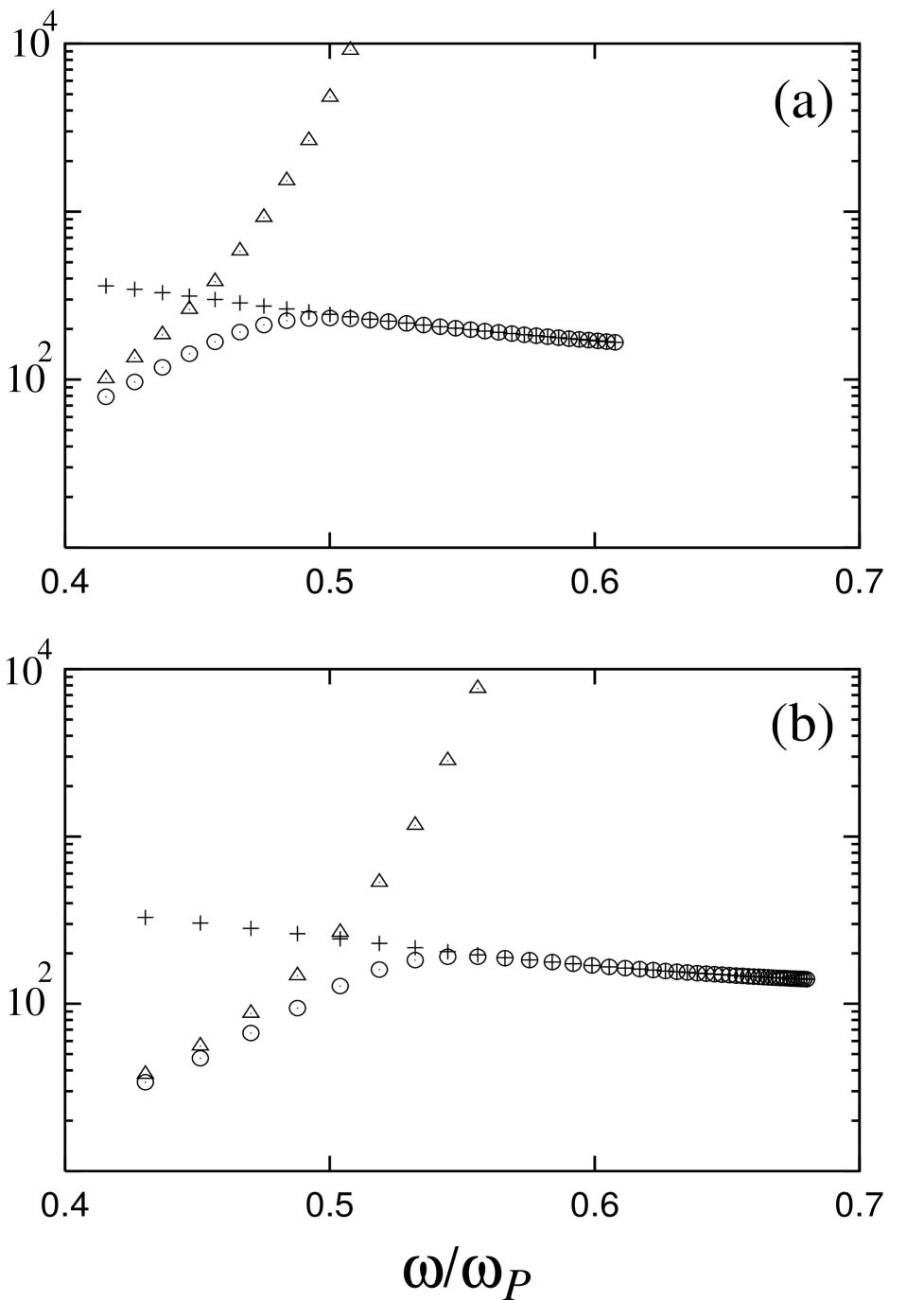
FIG. 14.: Quality factors $Q_{rad}$ ($\triangle$), $Q_{abs}$ (+), and $Q_{tot}$ ($\circ$) of TM_l SG field resonances in a metallic microsphere of complex $\epsilon(\omega)$ [Eq. (1), $\omega_{T}$ $\!=$ $\!0$, $\gamma/\omega_{P}$ $\!=$ $\!0.005$]. (a) $R$ $\!=$ $\!10\,\lambda_{P}$, $30$ $\!\leq$ $\!l$ $\!\leq$ $\!60$. (b) $R$ $\!=$ $\!5\,\lambda_{P}$, $16$ $\!\leq$ $\!l$ $\!\leq$ $\!60$. All resonances obey, in accordance with the condition (26), the relation $\omega/\omega_{P}$ $\!<$ $\!1/\sqrt{2}$ $\!\simeq$ $\!0.71$.

As a result, the radiative losses again dominate for low-order resonances and the absorption losses for high-order ones. Since absorption tends to be larger in metals than in dielectrics, the dominance of material absorption can already set in at lower-order resonances. Note that even for metals the relationship (8) typically still holds, so that Eqs. (24) – (27) apply.

The dependence of the decay rate on the transition frequency of an excited atom placed near a metallic microsphere is illustrated in Fig. 15(a) for a radially oriented transition dipole moment. An example of the emission pattern for the case when the atomic transition frequency coincides with the frequency of a SG wave is shown in Fig. 15(b). When the radius of the microsphere becomes too small, then SG waves cannot be excited. In particular, in [29] it was assumed that $R$ $\!\ll$ $\!\lambda_{P}$, and thus the resonances shown in Figs. 14 and 15(a) could not be found. It is worth noting that, in contrast to dielectric matter, a large absorption in metals can substantially

FIG. 15.: (a) Decay rate of an atom near a a metallic microsphere of complex permittivity $\epsilon(\omega)$ [Eq. (1), $\omega_{T}$ $\!=$ $\!0$, $\gamma/\omega_{P}$ $\!=$ $\!0.005$] as a function of the transition frequency for a radially oriented transition dipole moment ($R$ $\!=$ $\!5\lambda_{P}$, $\Delta r$ $\!=$ $\!0.1\,\lambda_{P}$). (b) Polar diagram of the normalized far-field emission pattern $|{\bf F}^{\perp}({\bf r},{\bf r}_{A},\omega_{A})|^{2}/(k_{A}^{3}\mu/4\pi\epsilon_{0})^{2}$ for $r$ $\!=$ $\!50\,\lambda_{P}$ and $\omega_{A}/\omega_{P}$ $\!=$ $\!0.5026$, the other parameters being the same as in (a).

enhance the near-surface divergence of the decay rate, [Eqs. (51) and (52)], which is in agreement with experimental observations of the fluorescence from a thin layer of optically excited organic-dye molecules that were separated from a planar metal surface by a dielectric layer of known thickness [30].

V Conclusions

We have applied the recently developed formalism [14] to the problem of spontaneous decay of an excited atom near a dispersing and absorbing microsphere. Basing the calculations on a complex permittivity of Drude-Lorentz type, which satisfies the Kramers-Kronig relations, we have been able to study the dependence of the decay rate on the transition frequency for arbitrary frequencies. We have shown that the decay can be substantially enhanced when the transition frequency is tuned to either a WG field resonance below the band gap (for a dielectric sphere) or a SG field resonance inside the band gap (for a dielectric sphere or a metallic sphere).

Whereas for both low-order WG field resonances and low-order SG field resonances radiative losses dominate, high-order field resonances mainly suffer from material absorption. Accordingly, spontaneous decay changes from being mainly radiative to being mainly nonradiative, when the transition frequency (tuned to a field resonance) in the respective frequency interval increases. We have further shown that in the presence of strong material absorption the decay rate drastically raises as the atom approaches the surface of the microsphere, because of near-field assisted energy transfer from the atom to the medium. Thus, the effect is typically observed for metals.

When radiative losses dominate, the emission pattern is highly structured, and a substantial fraction of the light is emitted backward and forward within small polar angles with respect to the tie line between the atom and the center of the sphere. With increasing absorption this directional characteristic is lost. When absorption losses dominate, the (weakened) emission pattern takes a form that is typical of reflection at a mirror.

In the paper we have restricted our attention to the weak-coupling regime, assuming that the excited atomic state decays exponentially. Obviously, when the atomic transition frequency coincides with a resonance frequency of the cavity-assisted field, the strong-coupling regime may be realized. In particular, SG waves seem to be best suited for that regime, because of the noticeable enhancement of spontaneous emission. The calculations could be performed in a similar way as in Ref. [14].

A The Green tensor

The Green tensor of a microsphere of radius $R$ (region 2) embedded in vacuum (region 1) can be decomposed into two parts [31],

$$\mathchoice{{\hbox{\boldmath$\displaystyle G$}}}{{\hbox{\boldmath$\textstyle G$}}}{{\hbox{\boldmath$\scriptstyle G$}}}{{\hbox{\boldmath$\scriptscriptstyle G$}}}({\bf r},{\bf r^{\prime}},\omega)=\mathchoice{{\hbox{\boldmath$\displaystyle G$}}}{{\hbox{\boldmath$\textstyle G$}}}{{\hbox{\boldmath$\scriptstyle G$}}}{{\hbox{\boldmath$\scriptscriptstyle G$}}}^{(s)}({\bf r},{\bf r^{\prime}},\omega)\delta_{fs}+\mathchoice{{\hbox{\boldmath$\displaystyle G$}}}{{\hbox{\boldmath$\textstyle G$}}}{{\hbox{\boldmath$\scriptstyle G$}}}{{\hbox{\boldmath$\scriptscriptstyle G$}}}^{(fs)}({\bf r},{\bf r^{\prime}},\omega),$$ (A1)

where $\mathchoice{{\hbox{\boldmath$\displaystyle G$}}}{{\hbox{\boldmath$\textstyle G$}}}{{\hbox{\boldmath$\scriptstyle G$}}}{{\hbox{\boldmath$\scriptscriptstyle G$}}}^{(s)}({\bf r},{\bf r^{\prime}},\omega)$ represents the contribution of the direct waves from the source in an unbounded space, and $\mathchoice{{\hbox{\boldmath$\displaystyle G$}}}{{\hbox{\boldmath$\textstyle G$}}}{{\hbox{\boldmath$\scriptstyle G$}}}{{\hbox{\boldmath$\scriptscriptstyle G$}}}^{(fs)}({\bf r},{\bf r^{\prime}},\omega)$ is the scattering part that describes the contribution of the multiple reflection ($f$ $\!=$ $\!s$) and transmission ($f$ $\!\neq$ $\!s$) waves ($f$ and $s$, respectively, refer to the regions where are the field and source points ${\bf r}$ and ${\bf r}^{\prime}$). In particular, $\mathchoice{{\hbox{\boldmath$\displaystyle G$}}}{{\hbox{\boldmath$\textstyle G$}}}{{\hbox{\boldmath$\scriptstyle G$}}}{{\hbox{\boldmath$\scriptscriptstyle G$}}}^{(s)}$, $\mathchoice{{\hbox{\boldmath$\displaystyle G$}}}{{\hbox{\boldmath$\textstyle G$}}}{{\hbox{\boldmath$\scriptstyle G$}}}{{\hbox{\boldmath$\scriptscriptstyle G$}}}^{(11)}$, and $\mathchoice{{\hbox{\boldmath$\displaystyle G$}}}{{\hbox{\boldmath$\textstyle G$}}}{{\hbox{\boldmath$\scriptstyle G$}}}{{\hbox{\boldmath$\scriptscriptstyle G$}}}^{(22)}$ can be given by [31]

$$\mathchoice{{\hbox{\boldmath$\displaystyle G$}}}{{\hbox{\boldmath$\textstyle G$}}}{{\hbox{\boldmath$\scriptstyle G$}}}{{\hbox{\boldmath$\scriptscriptstyle G$}}}^{(s)}({\bf r},{\bf r}^{\prime},\omega)={{\bf e}_{r}{\bf e}_{r}\over k_{s}^{2}}\delta(r-r^{\prime})$$ (A5)

$$\hskip 8.61108pt+{ik_{s}\over 4\pi}\sum_{e\atop o}\sum_{l=1}^{\infty}\sum_{m=0}^{l}{2l+1\over l(l+1)}{(l-m)!\over(l+m)!}\,(2\!-\!\delta_{0m})$$

$$\hskip 8.61108pt\times\left[{\bf M}^{(1)}_{{e\atop o}lm}({\bf r},k_{s}){\bf M}_{{e\atop o}lm}({\bf r}^{\prime},k_{s})\right.$$

$$\hskip 17.22217pt\left.+\,{\bf N}^{(1)}_{{e\atop o}lm}({\bf r},k_{s}){\bf N}_{{e\atop o}lm}({\bf r}^{\prime},k_{s})\right]$$

if $r$ $\!\geq$ $\!r^{\prime}$, and $\mathchoice{{\hbox{\boldmath$\displaystyle G$}}}{{\hbox{\boldmath$\textstyle G$}}}{{\hbox{\boldmath$\scriptstyle G$}}}{{\hbox{\boldmath$\scriptscriptstyle G$}}}^{(s)}({\bf r},{\bf r}^{\prime},\omega)$ $\!=$ $\!\mathchoice{{\hbox{\boldmath$\displaystyle G$}}}{{\hbox{\boldmath$\textstyle G$}}}{{\hbox{\boldmath$\scriptstyle G$}}}{{\hbox{\boldmath$\scriptscriptstyle G$}}}^{(s)}({\bf r}^{\prime},{\bf r},\omega)$ if $r$ $\!<$ $\!r^{\prime}$,

$$\mathchoice{{\hbox{\boldmath$\displaystyle G$}}}{{\hbox{\boldmath$\textstyle G$}}}{{\hbox{\boldmath$\scriptstyle G$}}}{{\hbox{\boldmath$\scriptscriptstyle G$}}}^{(11)}({\bf r},{\bf r^{\prime}},\omega)$$ (A9)

$$\hskip 8.61108pt={ik_{1}\over 4\pi}\sum_{e\atop o}\sum_{l=1}^{\infty}\sum_{m=0}^{l}{2l+1\over l(l+1)}{(l-m)!\over(l+m)!}\,(2\!-\!\delta_{0m})$$

$$\hskip 8.61108pt\times\Bigl{[}{\cal B}^{M}_{l}(\omega){\bf M}^{(1)}_{{e\atop o}lm}({\bf r},k_{1}){\bf M}^{(1)}_{{e\atop o}lm}({\bf r}^{\prime},k_{1})$$

$$\hskip 8.61108pt+\;{\cal B}^{N}_{l}(\omega){\bf N}^{(1)}_{{e\atop o}lm}({\bf r},k_{1}){\bf N}^{(1)}_{{e\atop o}lm}({\bf r}^{\prime},k_{1})\Bigr{]}$$

($r,r^{\prime}$ $\!>$ $\!R$),

$$\mathchoice{{\hbox{\boldmath$\displaystyle G$}}}{{\hbox{\boldmath$\textstyle G$}}}{{\hbox{\boldmath$\scriptstyle G$}}}{{\hbox{\boldmath$\scriptscriptstyle G$}}}^{(22)}({\bf r},{\bf r^{\prime}},\omega)$$ (A13)

$$\hskip 8.61108pt={ik_{2}\over 4\pi}\sum_{e\atop o}\sum_{l=1}^{\infty}\sum_{m=0}^{l}{2l+1\over l(l+1)}{(l-m)!\over(l+m)!}\,(2\!-\!\delta_{0m})$$

$$\hskip 8.61108pt\times\Bigl{[}{\cal C}^{M}_{l}(\omega){\bf M}_{{e\atop o}lm}({\bf r},k_{2}){\bf M}_{{e\atop o}lm}({\bf r}^{\prime},k_{2})$$

$$\hskip 8.61108pt+\;{\cal C}^{N}_{l}(\omega){\bf N}_{{e\atop o}lm}({\bf r},k_{2}){\bf N}_{{e\atop o}lm}({\bf r}^{\prime},k_{2})\Bigr{]}$$

($r,r^{\prime}$ $\!<$ $\!R$), where

$$k_{1}={\omega\over c},\qquad k_{2}=\sqrt{\epsilon(\omega)}\,{\omega\over c}\,.$$ (A14)

${\bf M}$ and ${\bf N}$ represent TE and TM waves, respectively,

$${\bf M}_{{e\atop o}lm}({\bf r},k)=\mp{m\over\sin\theta}j_{l}(kr)P_{l}^{m}(\cos\theta){\sin\choose\cos}(m\phi){\bf e}_{\theta}$$ (A16)

$$\hskip 51.6665pt-\,j_{l}(kr)\frac{dP_{l}^{m}(\cos\theta)}{d\theta}{\cos\choose\sin}(m\phi){\bf e}_{\phi}\,,$$

$${\bf N}_{{e\atop o}lm}({\bf r},k)={l(l\!+\!1)\over kr}j_{l}(kr)P_{l}^{m}(\cos\theta){\cos\choose\sin}(m\phi){\bf e}_{r}$$ (A19)

$$\hskip 51.6665pt+\,{1\over kr}\frac{d[rj_{l}(kr)]}{dr}\Biggl{[}\frac{dP_{l}^{m}(\cos\theta)}{d\theta}{\cos\choose\sin}(m\phi){\bf e}_{\theta}$$

$$\hskip 51.6665pt\mp\,{m\over\sin\theta}P_{l}^{m}(\cos\theta){\sin\choose\cos}(m\phi){\bf e}_{\phi}\Biggr{]},$$

with $j_{l}(x)$ and $P_{l}^{m}(x)$ being respectively the spherical Bessel function of the first kind and the associated Legendre function. The superscript ${(1)}$ in Eqs. (A5) and (A9) indicates that in Eqs. (A16) and (A19) the spherical Bessel function $j_{l}(x)$ has to be replaced by the first-type spherical Hankel function $h^{(1)}_{l}(x)$. The coefficients ${\cal B}^{M,N}_{l}$ and ${\cal C}^{M,N}_{l}$ in Eqs. (A9) and (A9) are defined by

$${\cal B}^{M}_{l}(\omega)$$ (A21)

$$\hskip 8.61108pt=-\frac{\bigl{[}z_{2}j_{l}(z_{2})\bigr{]}^{\prime}j_{l}(z_{1})-\bigl{[}z_{1}j_{l}(z_{1})\bigr{]}^{\prime}j_{l}(z_{2})}{\bigl{[}z_{2}j_{l}(z_{2})\bigr{]}^{\prime}h_{l}^{(1)}(z_{1})-j_{l}(z_{2})\bigl{[}z_{1}h_{l}^{(1)}(z_{1})\bigr{]}^{\prime}}\,,$$

$${\cal B}^{N}_{l}(\omega)$$ (A23)

$$\hskip 8.61108pt=-\frac{\epsilon(\omega)j_{l}(z_{2})\bigl{[}z_{1}j_{l}(z_{1})\bigr{]}^{\prime}-j_{l}(z_{1})\bigl{[}z_{2}j_{l}(z_{2})\bigr{]}^{\prime}}{\epsilon(\omega)j_{l}(z_{2})\bigl{[}z_{1}h_{l}^{(1)}(z_{1})\bigr{]}^{\prime}-\bigl{[}z_{2}j_{l}(z_{2})\bigr{]}^{\prime}h_{l}^{(1)}(z_{1})}\,,$$

$${\cal C}^{M}_{l}(\omega)$$ (A25)

$$\hskip 4.30554pt=-\frac{\bigl{[}z_{2}h_{l}^{(1)}(z_{2})\bigr{]}^{\prime}h_{l}^{(1)}(z_{1})-\bigl{[}z_{1}h_{l}^{(1)}(z_{1})\bigr{]}^{\prime}h_{l}^{(1)}(z_{2})}{\bigl{[}z_{2}j_{l}(z_{2})\bigr{]}^{\prime}h_{l}^{(1)}(z_{1})-j_{l}(z_{2})\bigl{[}z_{1}h_{l}^{(1)}(z_{1})\bigr{]}^{\prime}}\,,$$

$${\cal C}^{N}_{l}(\omega)$$ (A27)

$$=-\frac{\epsilon(\omega)h_{l}^{(1)}(z_{2})\bigl{[}z_{1}h_{l}^{(1)}(z_{1})\bigr{]}^{\prime}-h_{l}^{(1)}(z_{1})\bigl{[}z_{2}h_{l}^{(1)}(z_{2})\bigr{]}^{\prime}}{\epsilon(\omega)j_{l}(z_{2})\bigl{[}z_{1}h_{l}^{(1)}(z_{1})\bigr{]}^{\prime}-\bigl{[}z_{2}j_{l}(z_{2})\bigr{]}^{\prime}h_{l}^{(1)}(z_{1})}\,,$$

where

$$z_{i}=k_{i}R\ .$$ (A29)

Note that the relations

$$\int_{-1}^{1}dx\,P^{n}_{l}(x)P^{n}_{m}(x)=\frac{(l+n)!}{(l-n)!(l+1/2)}\,\delta_{lm}$$ (A30)

and

$$h^{(1)}_{l}(z)\rightarrow z^{-1}\exp\!\left[i(z\!-\!l\pi/2\!-\!\pi/4)\right]\quad{\rm if}\quad|z|\rightarrow\infty$$ (A31)

are valid [27].

B SG field resonances

For large value of $\nu$ $\!=$ $\!l+1/2$ the following asymptotic expansions are valid [27]:

$$J_{\nu}(nx)\sim{\exp[\nu(\tanh\alpha\!-\!\alpha)]\over\sqrt{2\pi\nu\tanh\alpha}}\left[1\!+\!\sum_{k=1}^{\infty}{u_{k}(\coth\alpha)\over\nu^{k}}\right]\!,$$ (B1)

$$Y_{\nu}(x)\sim-{\exp[\nu(\beta\!-\!\tanh\beta)]\over\sqrt{{1\over 2}\pi\nu\tanh\beta}}$$ (B3)

$$\hskip 43.05542pt\times\,\left[1+\sum_{k=1}^{\infty}(-1)^{k}{u_{k}(\coth\beta)\over\nu^{k}}\right]\!,$$

$$J^{\prime}_{\nu}(nx)\sim\sqrt{{\sinh 2\alpha\over 4\pi\nu}}\,\exp[\nu(\tanh\alpha-\alpha)]$$ (B5)

$$\hskip 43.05542pt\times\,\left[1+\sum_{k=1}^{\infty}{v_{k}(\coth\alpha)\over\nu^{k}}\right]\!,$$

$$Y^{\prime}_{\nu}(x)\sim\sqrt{{\sinh 2\beta\over\pi\nu}}e^{\nu(\beta-\tanh\beta)}$$ (B7)

$$\hskip 43.05542pt\times\,\left[1+\sum_{k=1}^{\infty}(-1)^{k}{v_{k}(\coth\beta)\over\nu^{k}}\right]\!,$$

[$Y_{\nu}(x)$ - Neumann function], where

$$\displaystyle x={\omega\over c}R,$$ (B8)

$$\displaystyle\cosh\alpha={\nu\over nx},\quad\cosh\beta={\nu\over x}\,,$$ (B9)

and $u_{k}$ and $v_{k}$ are given in Ref. [27]. To find the leading terms in Eqs. (10) and (12), we thus may write

$${J^{\prime}_{\nu}(nx)\over J_{\nu}(nx)}\sim|\sinh\alpha|,$$ (B10)

and

$${H^{\prime}_{\nu}(x)\over H_{\nu}(x)}\sim{Y^{\prime}_{\nu}(x)\over Y_{\nu}(x)}\sim-|\sinh\beta|$$ (B11)

to obtain,

$$\sqrt{\nu^{2}-x^{2}}+\sqrt{\nu^{2}-\epsilon x^{2}}=0$$ (B12)

for TE waves, and

$$\epsilon\sqrt{\nu^{2}-x^{2}}+\sqrt{\nu^{2}-\epsilon x^{2}}=0$$ (B13)

for TM waves. Here we have used relationships (B9), and we have assumed that $x$ scales as $\nu$ to discard the last term in Eq. (12).

Obviously, Eq. (B12) for TE waves has no solution, except for the trivial case of $\epsilon$ $\!=$ $1$. Equation (B13) for TM waves can be rewritten as

$$x=\nu\sqrt{1+\epsilon^{-1}}\,,$$ (B14)

which just implies condition (25). The higher-order corrections can be obtained by writing

$$x=\nu\sqrt{1+\epsilon^{-1}}\left[1+\sum_{k=1}^{\infty}{c_{k}\over\nu^{k}}\right],$$ (B15)

expanding all the quantities in Eq. (12) in powers of $\nu^{-1}$ and identifying the corresponding terms.

C Near-surface limit

Using the asymptotic Bessel-function expansion [27]

$$J_{\nu}(z)\sim{1\over\sqrt{2\pi\nu}}\left(ez\over 2\nu\right)^{\nu}\!,\quad Y_{\nu}(z)\sim-{2\over\sqrt{\pi\nu}}\left(ez\over 2\nu\right)^{-\nu}\!,$$ (C1)

($|\nu|$ $\!\gg$ $\!1$), the coefficient ${\cal B}^{N}_{l}(\omega_{A})$, Eq. (A23), can be given in the form of

$${\cal B}^{N}_{l}(\omega_{A})\left[h^{(1)}_{l}({k_{A}r_{A}})\over{k_{A}r_{A}}\right]^{2}$$ (C3)

$$\hskip 8.61108pt\sim{1\over i({k_{A}r_{A}})^{3}(2l+1)}{\epsilon(\omega_{A})-1\over\epsilon(\omega_{A})+1}\left(R\over r_{A}\right)^{2l+1}.$$

When the atom is located very close to the surface of the microsphere, i.e., $r_{A}$ $\!\gtrsim$ $\!R$, then from Eq. (C3) it follows that the series in Eq. (46) converges very slowly. Hence, it is a good approximation to apply equation (C3) to the terms with small $l$ as well. In this way, we derive

$$\sum_{l=1}^{\infty}l(l+1)(2l+1){\cal B}^{N}_{l}(\omega_{A})\left[h^{(1)}_{l}({k_{A}r_{A}})\over{k_{A}r_{A}}\right]^{2}$$ (C5)

$$\hskip 64.58313pt\sim\,{1\over 4i}{\epsilon(\omega_{A})-1\over\epsilon(\omega_{A})+1}{1\over(\Delta r)^{3}}\,.$$

Substitution of this expression into Eq. (46) then yields the leading term in Eq. (51). The leading term in Eq. (52) can be derived in a similar fashion.

REFERENCES

• [1] on leave from the Institute of Physics, National Center for Sciences and Technology, 1 Mac Dinh Chi Street, District 1, Ho Chi Minh city, Vietnam.
• [2] Optical Processes in Microcavities, edited by R. K. Chang and A. J. Campillo (World Scientific, Singapore, 1996).
• [3] L. Collot, V. Lefèvre-Seguin, M. Brune, J. M. Raimond and S. Haroche, Euro. Phys. Lett. 23, 327 (1993).
• [4] M. L. Gorodetsky, A. A. Savchenkov, and V. S. Ilchenko, Opt. Lett. 21, 453 (1996).
• [5] D. W. Vernooy, V. S. Ilchenko, H. Mabuchi, E. W. Streed, and H. J. Kimble, Opt. Lett. 23, 247 (1998).
• [6] S. Uetake, M. Katsuragawa, M. Suzuki, and K. Hakuta, Phys. Rev. 61, 011803 (1999).
• [7] E. M. Purcell, Phys. Rev. 69, 681 (1946).
• [8] H-B. Lin, J. D. Eversole, C. D. Merritt, and A. J. Campillo, Phys. Rev. A 45, 6756 (1992). H. Fujiwara, K. Sasaki, and H. Masuhara, J. Appl. Phys. 85, 2052 (1999); H. Yukawa, S. Arnold, and K. Miyano, Phys. Rev. A 60, 2491 (1999).
• [9] D. W. Vernooy, A. Furusawa, N. Ph. Georgiades, V. S. Ilchenko, and H. J. Kimble, Phys. Rev. A 57, R2293 (1998).
• [10] M. D. Barnes, C-Y. Kung, W. B. Whitten, J. M. Ramsey, S. Arnold, and S. Holler, Phys. Rev. Lett. 76, 3931 (1996); N. Lermer, M. D. Barnes, C-Y. Kung, W. B. Whitten, J. M. Ramsey, and S. C. Hill, Opt. Lett. 23, 951 (1998).
• [11] H. Chew, J. Chem. Phys. 87, 1355 (1987).
• [12] V. V. Klimov, M. Ducloy, and V. S. Letokhov, J. Mod. Opt. 43, 2251 (1996).
• [13] M. Pelton and Y. Yamamoto, Phys. Rev. A 59, 2418 (1999); O. Benson and Y. Yamamoto, ibid. 59, 4756 (1999).
• [14] S. Scheel, L. Knöll, and D.-G. Welsch, Phys. Rev. A 60, 4094 (1999); Ho Trung Dung, L. Knöll, and D.-G. Welsch, ibid. 62, 053804 (2000).
• [15] L. Knöll, S. Scheel, and D.-G. Welsch, in Coherence and Statistics of Photons and Atoms, edited by J. Perina (John Wiley & Son, New York, to be published), e-print quant-ph/0006121.
• [16] Ho Trung Dung, L. Knöll, and D.-G. Welsch, Phys. Rev. A 57, 3931 (1998); S. Scheel, L. Knöll, and D.-G. Welsch, ibid. 58, 700 (1998).
• [17] V. V. Klimov, M. Ducloy, and V. S. Letokhov, Phys. Rev. A, 59, 2996 (1999).
• [18] S. Schiller and R. L. Byer, Opt. Lett. 16, 1138 (1991); C. C. Lam, P. T. Leung, and K. Young, J. Opt. Soc. Am. B 9, 1585 (1992).
• [19] S. Arnold and L. M. Folan, Opt. Lett. 14, 387 (1989).
• [20] P. Chýlek, H-B. Lin, J. D. Eversole, and A. J. Campillo, Opt. Lett. 16, 1723 (1991).
• [21] H. Raether, Surface Plasmons on Smooth and Rough Surfaces and on Gratings (Springer-Verlag, Berlin, 1988).
• [22] P. W. Milonni, The Quantum Vacuum: An Introduction to Quantum Electrodynamics (Academic, San Diego, 1994).
• [23] M. S. Yeung and T. K. Gustafson, Phys. Rev. A 54, 5227 (1996).
• [24] S. Scheel, L. Knöll, and D.-G. Welsch, Acta Phys. Slov. 49, 585 (1999).
• [25] S. C. Ching, H. M. Lai, and K. Young, J. Opt. Soc. Am. B 4, 2004 (1987).
• [26] Higher Transcendental Functions, edited by A. Erdélyi (McGraw-Hill, New York, 1953).
• [27] Handbook of Mathematical Functions, edited by A. Abramovitz and I. A. Stegun (Dover, New York, 1973).
• [28] D. J. Nash and J. R. Sambles, J. Mod. Opt. 43, 81 (1996).
• [29] R. Ruppin, J. Chem. Phys. 76, 1681 (1982).
• [30] K. H. Drexhage, Progress in Optics XII, edited by E. Wolf (North-Holland, Amsterdam, 1974), p. 165.
• [31] L. W. Li, P. S. Kooi, M. S. Leong, and T. S. Yeo, IEEE Trans. Microwave Theory Tech. 42, 2302 (1994).