Separability properties of tripartite states with $\rm U\!\otimes\!U\!\otimes\!U$-symmetry

Abstract

We study separability properties in a $5$-dimensional set of states of quantum systems composed of three subsystems of equal but arbitrary finite Hilbert space dimension. These are the states, which can be written as linear combinations of permutation operators, or, equivalently, commute with unitaries of the form $U\otimes U\otimes U$. We compute explicitly the following subsets and their extreme points: (1) triseparable states, which are convex combinations of triple tensor products, (2) biseparable states, which are separable for a twofold partition of the system, and (3) states with positive partial transpose with respect to such a partition. Tripartite entanglement is investigated in terms of the relative entropy of tripartite entanglement and of the trace norm.

I Introduction

One of the difficulties in the theory of entanglement is that state spaces are usually fairly high dimensional convex sets. Therefore, to explore in detail the potential of entangled states one often has to rely on lower dimensional “laboratories”. An example of this was the role played by a one-dimensional family of bipartite states [1], which has come to be known as “Werner states”. In this paper we present a similar laboratory, designed for the study of entanglement between three subsystems. The basic idea is rather similar to [1], and we believe this set shares many of the virtues with its bipartite counterpart. Firstly, the states have an explicit parameterization as linear combinations of permutation operators. This is helpful for explicit computations. Secondly, there is a “twirl” operation which brings an arbitrary tripartite state to this special subset. This proved to be very helpful for the discussion of entanglement distillation of bipartite entanglement: the first useful distillation procedures worked by starting with Werner states, applying a suitable distillation operation, and then the twirl projection to come back to the simple and well understood subset, thus allowing iteration [2, 3]. Geometrically this means that the subset we investigate is both a section of the state space by a plane and the image of the state space under a projection. The basic technique for getting such subsets is averaging over a symmetry group of the entire state space. Such an averaging projection preserves separability if it is an average only over local (factorizing) unitaries. Of course, special subgroups might turn out to be useful. For example, in a recent paper [4] a class of tripartite ($n=3$) states was studied for dimension $d=2,$ which is invariant under unitaries of the group of order 24 generated by $\sigma_{1}^{\otimes 3},$ $\sigma_{3}\otimes{\openone}\otimes\sigma_{3},$ ${\openone}\otimes\sigma_{3}\otimes\sigma_{3}$ and $\exp(i\pi\sigma_{3}/3)^{\otimes 3}.$

The third useful property of the states we study is that they can be defined for systems of arbitrary finite Hilbert space dimension $d$, leading to the same $5$-dimensional convex set for every $d$. (This generalizes to an $(n!-1)$-dimensional set for $n$-partite systems). Surprisingly, it turns out that the separability sets we investigate are also independent of dimension.

We now describe the natural entanglement (or separability) properties we will chart for these special states. Our classification is similar to the one used in [4], but differs in that we do not artificially make the classes disjoint.

Of course, we can split the system into just two subsystems and apply the usual separability/entanglement distinctions. A split $1|23$ then corresponds to the grouping of the Hilbert space ${\cal H}_{1}\otimes{\cal H}_{2}\otimes{\cal H}_{3}$ into ${\cal H}_{1}\otimes({\cal H}_{2}\otimes{\cal H}_{3})$. We call a density operator $\rho$ on this Hilbert space $1|23$-separable, or just biseparable if the partition is clear from the context, if we can write

$$\rho=\sum_{\alpha}\lambda_{\alpha}\ \rho^{(1)}_{\alpha}\otimes\rho^{(23)}_{\alpha},$$ (1)

with $\lambda_{\alpha}\geq 0$ and density operators $\rho^{(23)}_{\alpha}$ on ${\cal H}_{2}\otimes{\cal H}_{3}$. We will denote the set of such $\rho$ by ${\cal B}_{1}$. This set will be computed in Section V. Furthermore, as it is a necessary condition for biseparability (cf. Peres [5]), we are going to look at those states $\rho$ having a positive partial transpose with regard to such a split, denoted by $\rho\in{\cal P}_{1}$. Recall that the partial transpose $A\mapsto A^{T_{1}}$ of operators on ${\cal H}_{1}\otimes{\cal H}_{2}$ is defined by

$$(\sum_{\alpha}A_{\alpha}\otimes B_{\alpha})^{T_{1}}=\sum_{\alpha}A_{\alpha}^{T}\otimes B_{\alpha},$$ (2)

where $A^{T}$ on the right hand side is the ordinary transposition of matrices with respect to a fixed basis. It is clear that ${\cal B}_{1}\subset{\cal P}_{1}$ holds, but as we will show in Section VI by computing ${\cal P}_{1}$, this inclusion is strict except for $d=2$.

As a genuinely “tripartite” notion of separability, we consider states, called triseparable (or “three-way classically correlated”), which can be decomposed as

$$\rho=\sum_{\alpha}\lambda_{\alpha}\ \rho^{(1)}_{\alpha}\otimes\rho^{(2)}_{\alpha}\otimes\rho^{(3)}_{\alpha},$$ (3)

where $\lambda_{\alpha}\geq 0$, and the $\rho^{(i)}_{\alpha}$ are density operators on the respective Hilbert spaces. The set of such density operators will be denoted by ${\cal T}$. Of course, we may also consider states which are biseparable for all three partitions. It is known [6] that this does not imply triseparability, i.e. ${\cal T}\subsetneqq({\cal B}_{1}\cap{\cal B}_{2}\cap{\cal B}_{3})$. Further examples will be found below.

Since in this paper we will only be interested in a five dimensional set ${\cal W}$ of symmetric states (see the next section), we will from now on use the symbols ${\cal T},{\cal B}_{1}$ and ${\cal P}_{1}$ only for the corresponding subsets of ${\cal W}$.

II Definition and Main Results

A $U\otimes U\otimes U$-invariant states: ${\cal W}$

Throughout we consider states on a Hilbert space of the form ${\cal H}\otimes{\cal H}\otimes{\cal H}$, where ${\cal H}$ is a Hilbert space of finite dimension $d$. The group of permutations on $3$ elements acts on this space by unitary operators $V_{\pi}$, defined by

$$V_{\pi}\ \phi_{1}\otimes\phi_{2}\otimes\phi_{3}=\phi_{\pi^{-1}1}\otimes\phi_{\pi^{-1}2}\otimes\phi_{\pi^{-1}3}.$$

For the six permutations $\pi$ we use cycle notation, so that $V_{(12)}$ is the permutation operator of the first two factors, and $V_{(123)}$ is the cyclic permutation taking $1$ to $2$. We denote by “$dU$” the normalized Haar measure on the unitary group of ${\cal H}$, and define on the space of operators the operator

$${\bf P}\rho=\int\!dU\ (U\otimes U\otimes U)\rho\,(U\otimes U\otimes U)^{*}.$$ (4)

Clearly, ${\bf P}$ takes positive operators to positive operators (it is even completely positive), and $\mathop{\rm tr}\nolimits({\bf P}\rho)=\mathop{\rm tr}\nolimits(\rho)$, i.e., ${\bf P}$ maps density operators to density operators. We can now define the set of states, which form the object of our investigation.

Lemma 1

For an operator $\rho$ on ${\cal H}\otimes{\cal H}\otimes{\cal H}$ the following conditions are equivalent:

1. $(U\otimes U\otimes U)\rho=\rho(U\otimes U\otimes U)$ for all unitary operators $U$ on ${\cal H}$.

2. ${\bf P}\rho=\rho$.

3. $\rho=\sum_{\pi}\mu_{\pi}V_{\pi}$ with coefficients $\mu_{\pi}\in{\mathbb{C}}$.

The set of density operators satisfying these conditions will be denoted by ${\cal W}$.

The equivalence of (1) and (2) is straightforward from the invariance of the Haar measure. The implication (3)$\Longrightarrow$(1) is trivial, because the permutation operators clearly commute with operators of the form $(U\otimes U\otimes U)$. The only non-trivial part is thus (1)$\Longrightarrow$(3) which is, however, a standard result ( [7] chap.IV) from representation theory. Of course, all this works for any number of tensor factors.

The above Lemma does not address the question how to recognize density matrices in terms of the six coefficients $\mu_{\pi}$. Hermiticity requires $\mu_{\pi^{-1}}=\overline{\mu_{\pi}}$, leaving effectively six real parameters. One more is fixed by normalization, so that ${\cal W}$ is embedded in a five dimensional real vector space. In terms of the parameters $\mu_{\pi}$ positivity is not easy to see. In order to get a better criterion it is best to study the algebra of operators, which are linear combinations of the permutations. The product of such operators can readily be computed by using only the multiplication law for permutations. The abstract algebra of formal linear combinations of group elements (known as the group algebra) can be decomposed in terms of the irreducible representations of the underlying group, suggesting a basis which is much more handy for deciding positivity. Again this step works for any number of factors, but we carry it out only in the case $n=3$: We introduce the following linear combinations of permutation operators:

$$R_{+}\! = \frac{1}{6}\bigl{(}{\openone}+V_{(12)}+V_{(23)}+V_{(31)}+V_{(123)}+V_{(321)}\bigr{)}$$ (6)

$$R_{-}\! = \frac{1}{6}\bigl{(}{\openone}-V_{(12)}-V_{(23)}-V_{(31)}+V_{(123)}+V_{(321)}\bigr{)}$$ (7)

$$R_{0} = \frac{1}{3}\Bigl{(}2\cdot{\openone}-V_{(123)}-V_{(321)}\Bigr{)}$$ (8)

$$R_{1} = \frac{1}{3}\Bigl{(}2V_{(23)}-V_{(31)}-V_{(12)}\Bigr{)}$$ (9)

$$R_{2} = \frac{1}{\sqrt{3}}\ \Bigl{(}V_{(12)}-V_{(31)}\Bigr{)}$$ (10)

$$R_{3} = \frac{i}{\sqrt{3}}\ \Bigl{(}V_{(123)}-V_{(321)}\Bigr{)}.$$ (11)

Then $R_{+},R_{-},R_{0}$ are orthogonal projections adding up to ${\openone}$, and commute with all permutations. This means that they correspond to the irreducible representations of the permutation group: $R_{+}$ and $R_{-}$ correspond to the two one-dimensional representations (trivial and alternating representation respectively), and these operators are indeed just the orthogonal projections onto the symmetric and anti-symmetric subspaces of ${\cal H}\otimes{\cal H}\otimes{\cal H}$ in the usual sense. Their complement $R_{0}$ corresponds to a two dimensional representation, which is hence isomorphic to the $2\times 2$-matrices. The operators $R_{1},R_{2},R_{3}$ act as the Pauli matrices of this representation. In other words, the six hermitian operators $R_{+},R_{-},R_{0},R_{1},R_{2},R_{3}$ are characterized by the commutation relations $R_{i}R_{\pm}=R_{\pm}R_{i}=0$, $R_{i}^{2}=R_{0}$, for $i=0,1,2,3$, and $R_{1}R_{2}=iR_{3}$ with cyclic permutations.

Now every operator $\rho$ in the linear span of the permutations can be decomposed into the orthogonal parts $R_{+}\rho$, $R_{-}\rho$, and $R_{0}\rho$, and positivity of $\rho$ is equivalent to the positivity of all three operators. This leads to the following Lemma:

Lemma 2

For any operator $\rho$ on ${\cal H}\otimes{\cal H}\otimes{\cal H}$, define the six parameters $r_{k}(\rho)=\mathop{\rm tr}\nolimits(\rho R_{k})$, for $k\in\{+,-,0,1,2,3\}$. Then $r_{k}({\bf P}\rho)=r_{k}(\rho)$. Moreover, each $\rho\in{\cal W}$ is uniquely characterized by the tuple $(r_{+},r_{-},r_{0},r_{1},r_{2},r_{3})\in{\mathbb{R}}^{6}$, and such a tuple belongs to a density matrix $\rho\in{\cal W}$ if and only if

$$r_{+},r_{-},r_{0}\geq 0, r_{+}+r_{-}+r_{0}=1$$ (12)

$${\rm and} r_{1}^{2}+r_{2}^{2}+r_{3}^{2}\leq r_{0}^{2}.$$ (13)

Note that in this parameterization the set ${\cal W}$ does not depend on the dimension $d$ with one exception: for $d=2$ the anti-symmetric projection $R_{-}$ is simply zero, so for qubits we get the additional constraint $r_{-}=0$. If one considers a given density operator $\rho$ as an operator $\rho^{\prime}$ in ${\cal H}^{\prime}\otimes{\cal H}^{\prime}\otimes{\cal H}^{\prime}$ for a higher dimensional space ${\cal H}^{\prime}\supset{\cal H}$, by setting all “new” matrix elements equal to zero, we will have $r_{k}(\rho)=r_{k}(\rho^{\prime})$.

Taking $r_{0}=1-r_{+}-r_{-}$ to be redundant, we get a simple representation of ${\cal W}$ as a convex set in $5$ dimensions. Unfortunately, $5$ dimensional sets are still not very amenable to graphical representation. For visualizing the sets we are going to describe analytically, we will therefore use suitable $2$ and $3$ dimensional representations. Again, we have the possibility of using sections or projections of ${\cal W}$, and we will emphasize sections which can also be understood as projections.

The simplest example of this is to take the subset ${\cal W}^{P}\subset{\cal W}$ of states, which also commute with all permutations. The corresponding projection is simply averaging with respect to permutations. Clearly, ${\cal W}^{P}$ consists of those operators in ${\cal W}$, which are linear combinations of $R_{+},R_{-},R_{0}$ alone. Taking $r_{+}$ and $r_{-}$ as coordinates we get the triangle in Figure 1. Thus each point in this triangle represents a density operator in ${\cal W}^{P}$. On the other hand, it represents the set of states in ${\cal W}$ projecting to it on permutation averaging: this will be all states with the given values of $r_{+}$ and $r_{-}$ in the $6$-tuple, which therefore differ only in the values of $r_{1},r_{2}$, and $r_{3}$. Thus over every point of the triangle in Figure 1 we should imagine a Bloch sphere of radius $r_{0}$.

If more detail is required, we will also use three dimensional sections and/or projections of a similar nature. For example, if we average only over the permutations $V_{(23)}$, we get the subset ${\cal W}^{(23)}\subset{\cal W}$ with $r_{2}=r_{3}=0$ (see the dotted tetrahedron in Figure 10). Averaging only over cyclic permutations, we get the subset ${\cal W}^{\rm cyc}\subset{\cal W}$ with $r_{1}=r_{2}=0$ (which gives the same tetrahedron as ${\cal W}^{(23)}$ with $r_{1}$ substituted by $r_{3}.$).

We note for later use that the expectation values $r_{k}$ are not the coefficients in the sum

$$\rho=\sum_{k=+,-,0,1,2,3}c_{k}R_{k}.$$ (14)

These are related to the $r_{k}$ by the following dimension dependent transformation (which is obtained by observing that $\mathop{\rm tr}\nolimits{\openone}=d^{3}$, $\mathop{\rm tr}\nolimits(V_{(12)})=d^{2}$, and $\mathop{\rm tr}\nolimits(V_{(123)})=d$).

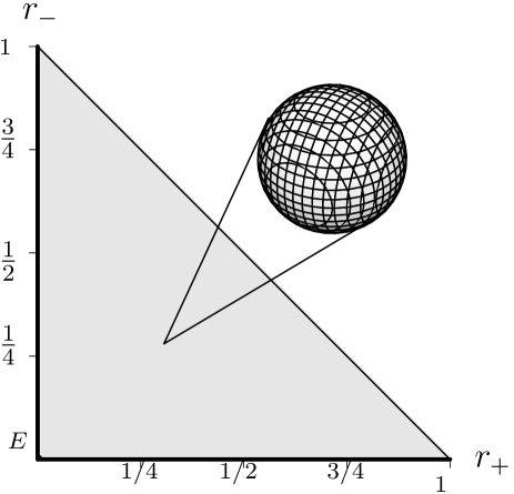
FIG. 1.: Description of ${\cal W}$ in terms of the triangle ${\cal W}^{P}$ and the corresponding Bloch sphere for each point in ${\cal W}^{P}.$

$$r_{+}\! = \frac{d}{6}(d^{2}+3d+2)\ c_{+}$$ (16)

$$r_{-}\! = \frac{d}{6}(d^{2}-3d+2)\ c_{-}$$ (17)

$$r_{i} = \frac{2d}{3}(d^{2}-1)\ c_{i}\quad{\rm for}\ i=0,1,2,3.$$ (18)

B Overview of Main Results

An overview of the main results of this paper is given in Figure 2. To keep the picture as simple as possible, we have only depicted the set ${\cal W}^{P}$, i.e., the triangle in Figure 1. Naturally, this reduction does not allow the representation of our full results, i.e., the detailed structure of the five-dimensional convex sets ${\cal T},{\cal B}_{1}$, and ${\cal P}_{1}$, which will be described in the corresponding sections. However, we found this diagram quite useful as a basic map for not losing our way in five dimensions, and hope it will similarly serve our readers.

The shading in Figure 2 marks different separability properties, and the points labeled with capital letters arise by projecting pure states with special properties with the twirl projection (4). Some of these points (D,E,F) do not lie in the plane ${\cal W}^{P}$, i.e, they have non-zero coordinates $(r_{1},r_{2},r_{3})$. They are represented by white circles, in contrast to the black circles (A,B,C,G,H) representing permutation invariant states in the plane ${\cal W}^{P}$.

The triseparable states correspond to the black triangle $\triangle$(ABC). It is easy to see that any triseparable state projected by permutation averaging to ${\cal W}^{P}$ is again triseparable, i.e., the projection of ${\cal T}$ onto ${\cal W}^{P}$ coincides with ${\cal T}\cap{\cal W}^{P}$. The extreme points of this set are

$$A: |123\rangle\longrightarrow(1/6,1/6,0,0,0)$$

$$B: |111\rangle\longrightarrow(1,0,0,0,0)$$

$$C: (|111\rangle-\sqrt{3}|112\rangle+\sqrt{3}|121\rangle-3|122\rangle)/4$$

$$\qquad\qquad\qquad\qquad\qquad\longrightarrow(1/4,0,0,0,0)\;,$$

where the notation $\Psi\longrightarrow(r_{+},r_{-},r_{1},r_{2},r_{3})$ indicates that the pure state $|\Psi\rangle\!\langle\Psi|$ is projected to this point by ${\bf P}$ from (4). In other words, $\langle\Psi|R_{k}\Psi\rangle=r_{k}$ for $k=+,-,1,2,3$. Note that all three vectors given are product vectors, the one for C being the product of three vectors in the “Mercedes star” configuration in the plane, at angle $120^{\circ}$ from each other.

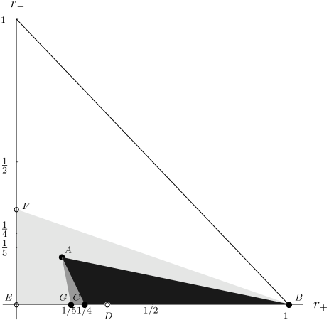
FIG. 2.: Subsets of ${\cal W}^{P}$ with different separability properties. Black: triseparable, dark grey: biseparable, light grey: images of biseparable states under permutation averaging. Special points explained in the text.

A quantitative description of the genuinely tripartite entanglement of ${\cal W}$ is given in section IV in terms of the relative entropy and the trace norm.

The biseparable set ${\cal B}_{1}$ is not permutation invariant, since the partition $1|23$ clearly is not. As a consequence, the permutation average projecting ${\cal W}$ onto ${\cal W}^{P}$ does not map ${\cal B}_{1}$ into itself, and we have to distinguish in our diagram between points $(r_{+},r_{-})$ such that $(r_{+},r_{-},0,0,0)$ is biseparable (i.e., the intersection ${\cal B}_{1}\cap{\cal W}^{P}$), and points $(r_{+},r_{-})$ such that for some suitable $(r_{1},r_{2},r_{3})$ the quintuple $(r_{+},r_{-},r_{1},r_{2},r_{3})$ represents a point in ${\cal B}_{1}$, (i.e., the projection of ${\cal B}_{1}$ onto ${\cal W}^{P}$). In Figure 2 the intersection is the triangle $\triangle$(GAB), drawn in a darker shade of grey than the triangle $\triangle$(EFB), which is the projection of the biseparable subset ${\cal B}_{1}$. Note that the shading reflects the inclusion relations, i.e., triseparable states are, in particular, biseparable, and the section of the biseparable set is contained in its projection. Of course, the states in ${\cal B}_{1}\cap{\cal W}^{P}$ are also biseparable for the other two partitions, since they are permutation invariant. Similarly, the projections of ${\cal B}_{2}$ and ${\cal B}_{3}$ onto ${\cal W}^{P}$ are the same.

Points of special interest for the biseparable set arise from the following vectors:

$$D: |122\rangle\longrightarrow(1/3,0,2/3,0,0)$$

$$E: (|112\rangle-|121\rangle)/\sqrt{2}\longrightarrow(0,0,-1,0,0)$$

$$F: (|123\rangle-|132\rangle)/\sqrt{2}\longrightarrow(0,1/3,-2/3,0,0)$$

$$G: (|112\rangle-|121\rangle-\sqrt{3}|122\rangle)/\sqrt{5}\longrightarrow(1/5,0,0,0,0)\;.$$

Here the points B,D,E, and F are extreme points of ${\cal B}_{1}$, and span a tetrahedron, which is equal to the subset ${\cal B}_{1}\cap{\cal W}^{(23)}$ of states invariant under the exchange $2\leftrightarrow 3$. The point G lies on the line connecting E and D, and is the unique extreme point of ${\cal B}_{1}\cap{\cal W}^{P}$ which is not triseparable. In this sense it represents an extreme case demonstrating the inequality ${\cal T}\neq({\cal B}_{1}\cap{\cal B}_{2}\cap{\cal B}_{3})$.

The set ${\cal P}_{1}$ of states with positive partial transpose with respect to the partition $1|23$ contains ${\cal B}_{1}$ strictly, but the difference cannot be seen in this diagram. In fact, we will show in Section VI that even the 23-invariant subsets of ${\cal P}_{1}$ and ${\cal B}_{1}$ coincide, i.e., ${\cal P}_{1}\cap{\cal W}^{(23)}$ is spanned by the same four extreme points B,D,E, and F.

As will be seen in Section VI there is a close connection between the problems of finding ${\cal P}_{1}$ and finding states invariant under averaging over all unitaries of the form $\overline{U}\otimes U\otimes U$. It turns out that the sets of triseparable and biseparable states commuting with such unitaries can be obtained via a simple linear transformation from their counterparts ${\cal T}\cap{\cal W}$ and ${\cal B}_{1}\cap{\cal W}$ computed in this paper. This mapping and a sketch of the results is given in the Appendix.

III Triseparable states: ${\cal T}$

If $\rho$ is triseparable, hence has a decomposition of the form (3), we may also find a decomposition in which all factors $\rho^{(i)}_{\alpha}$ are pure, simply by decomposing each of these density operators into pure ones. Applying to such a decomposition the projection ${\bf P}$ we find that $\rho\in{\cal T}\subset{\cal W}$ if and only if $\rho$ is a convex combination of states of the form ${\bf P}(|\Psi\rangle\!\langle\Psi|),$ where $\Psi=\psi_{1}\otimes\psi_{2}\otimes\psi_{3}$ is a normalized product vector. Let us denote by ${\cal T}_{\rm pure}\subset{\cal W}$ the set of such states. Our strategy for determining ${\cal T}$ will be to first get ${\cal T}_{\rm pure}$, and then to obtain ${\cal T}$ as its convex hull. The resulting characterization of ${\cal T}$ is formulated in Theorem 5.

Given a product vector $\Psi=\psi_{1}\otimes\psi_{2}\otimes\psi_{3}$, it is easy to compute the projected state ${\bf P}(|\Psi\rangle\!\langle\Psi|)$: By Lemma 2 one just has to compute the expectations of the permutation operators. For example,

$$\langle\Psi|V_{(12)}\Psi\rangle=\langle\psi_{1}\otimes\psi_{2}\otimes\psi_{3}|\psi_{2}\otimes\psi_{1}\otimes\psi_{3}\rangle=|\langle\psi_{1}|\psi_{2}\rangle|^{2}.$$

In this way it is easily seen that the expectations of all permutations are $\{1,a_{1},a_{2},a_{3},a_{4}+ia_{5},a_{4}-ia_{5}\}$, where the $5$ real parameters are given by

$$a_{1} = |\langle\psi_{2}|\psi_{3}\rangle|^{2}$$ (20)

$$a_{2} = |\langle\psi_{3}|\psi_{1}\rangle|^{2}$$ (21)

$$a_{3} = |\langle\psi_{1}|\psi_{2}\rangle|^{2}$$ (22)

$$a_{4} = \Re\!e\left(\langle\psi_{1}|\psi_{2}\rangle\langle\psi_{2}|\psi_{3}\rangle\langle\psi_{3}|\psi_{1}\rangle\right)$$ (23)

$$a_{5} = \Im\!m\left(\langle\psi_{1}|\psi_{2}\rangle\langle\psi_{2}|\psi_{3}\rangle\langle\psi_{3}|\psi_{1}\rangle\right).$$ (24)

Since a pure state in $d$ dimensions (taken up to a factor) is given by $2d-2$ real parameters, these $5$ quantities are a considerable reduction from the $6(d-1)$ parameters determining the three vectors $\psi_{i}$. However, they are still not independent, due to the identity

$$f(a_{1},a_{2},a_{3},a_{4},a_{5}):=a_{4}^{2}+a_{5}^{2}-a_{1}a_{2}a_{3}=0.$$ (25)

Since we want to determine ${\cal T}_{\rm pure}$ exactly, we also have to find the exact range of these parameters, as the $\psi_{i}$ vary over all unit vectors. This is done in the following Lemma.

Lemma 3

A tuple $(a_{1},a_{2},a_{3},a_{4},a_{5})\in{\mathbb{R}}^{5}$ arises via equations (III) from three unit vectors $\psi_{1},\psi_{2},\psi_{3}$ in a $d$-dimensional Hilbert space ($d>3$), if and only if equation (25) is satisfied, $0\leq a_{i}\leq 1$ for $i=1,2,3$, and

$$1-a_{1}-a_{2}-a_{3}+2a_{4}\geq 0.$$ (26)

If $d=2$ the Lemma holds with last inequality replaced by equality.

Proof: Necessity of equation (25), and $0\leq a_{i}\leq 1$ is clear. Inequality (26) is just the condition that the expectation of antisymmetric projection should be positive. Since this projection vanishes for $d=2$, it is also clear that equality must hold in this case.

Suppose now that $a_{1},\ldots,a_{5}$ satisfying these constraints are given. We have to reconstruct $\psi_{1},\psi_{2}$, and $\psi_{3}$ satisfying equations (III). These equations essentially determine the $3\times 3$-matrix $M_{ij}=\langle\psi_{i}|\psi_{j}\rangle$ of scalar products. Of course, we already know the absolute values of its entries (note $M_{ii}=1$). The phases are irrelevant up to some extent: multiplying any row with a phase, and the corresponding column with its complex conjugate will not change the $a_{i}$ after equation (III), and amounts to multiplying one of the $\psi_{i}$ with a phase. Hence we may assume that the scalar products $\langle\psi_{1}|\psi_{2}\rangle$ and $\langle\psi_{2}|\psi_{3}\rangle$ are positive. The phase of the remaining scalar product $\langle\psi_{3}|\psi_{1}\rangle$ is then the same as the phase of $a_{4}+ia_{5}$, hence $M$ is essentially uniquely determined by the $a_{i}$.

Now a matrix $M$ is a matrix of scalar products if and only if it is positive definite: on the one hand, $\sum_{ij}\overline{u_{i}}u_{j}M_{ij}=\|\sum_{i}u_{i}\psi_{i}\|^{2}\geq 0$. On the other hand, we can construct a Hilbert space with such scalar products as the space of formal linear combinations of three vectors, with scalar products of basis vectors defined by $M$. Positive definiteness of $M$ then ensures the positivity of the norm in this new Hilbert space. The dimension of this space is the rank of $M$ (number of linearly independent rows/columns). So in the present case the dimension will be $3$ (but any larger space will also contain appropriate vectors) or $\leq 2$, if $M$ is a singular matrix.

Positive definiteness of $M$ is equivalent to the positivity of all subdeterminants. The diagonal elements are $1$, hence positive anyway. Positivity of the three $2\times 2$ subdeterminants is equivalent to $a_{i}\leq 1$ for $i=1,2,3$. Finally, the full determinant of $M$, expressed in terms of the $a_{i}$ gives expression (26). It must be positive, and for $d=2$ it must vanish, since $M$ is singular.         

Lemma 3 describes the set ${\cal T}_{\rm pure}$ of projected pure product states as a compact subset of the hypersurface in ${\mathbb{R}}^{5}$ defined by equation (25). Computing the convex hull of this set in ${\mathbb{R}}^{5}$ is the same as computing the convex hull of ${\cal T}_{\rm pure}$, because the expectations of permutations or the operators $R_{k}$ from (1) are affine functions of the $a_{i}$. Explicitly, the expectations $r_{k}=\langle\Psi|R_{k}\Psi\rangle$, $k=+,-,0,1,2,3$, which we have used as our standard coordinates in ${\cal W}$ are

$$r_{+}\! = \frac{1}{6}\ (1+(a_{1}+a_{2}+a_{3})+2a_{4})$$

$$r_{-}\! = \frac{1}{6}\ (1-(a_{1}+a_{2}+a_{3})+2a_{4})$$

$$r_{0} = \frac{2}{3}(1-a_{4})$$

$$r_{1} = \frac{1}{3}\ (2a_{1}-a_{2}-a_{3})$$

$$r_{2} = \frac{1}{\sqrt{3}}\ (a_{3}-a_{2})$$

$$r_{3} = \frac{2}{\sqrt{3}}\ a_{5}.$$

We begin by computing the projection of ${\cal T}_{\rm pure}$ onto the $(r_{+},r_{-})$-plane, by determining the possible range of the combinations $m=(a_{1}+a_{2}+a_{3})/3$ and $a_{4}$. By choosing phases for the scalar products we can make $a_{4}$ vary in the range $|a_{4}|\leq(a_{1}a_{2}a_{3})^{1/2}=g^{3/2}$, where $m$ and $g$ are the arithmetic and the geometric mean of $a_{1},a_{2},a_{3}$. As is well known, $g\leq m$, and equality holds if $a_{1}=a_{2}=a_{3}$. Hence the projection of ${\cal T}_{\rm pure}$ is contained between the parameterized lines

$$r_{+}(m) = \frac{1}{6}(1+3m\pm 2m^{2/3})$$

$$r_{-}(m) = \frac{1}{6}(1-3m\pm 2m^{2/3})\;.$$

Plotting these curves gives Figure 3. It is clear that the shape is not convex, and its convex hull is the triangle $ABC$.

FIG. 3.: Section of the set ${\cal T}_{\rm pure}$ with ${\cal W}^{P}$ and its convex hull.

A similar plot of the set ${\cal T}_{\rm pure}$ including one more coordinate, $r_{3}$, is given in Figure 4.

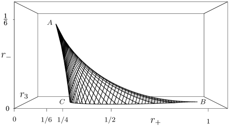
FIG. 4.: Plot of the same section as above making additional use of the coordinate $r_{3}.$

Again it is clear that no point on the surface can be an extreme point of the convex hull of the surface, because the surface “curves the wrong way”. This is the intuition behind the following Lemma, by which we will show that also in the full five-dimensional case the interior of ${\cal T}_{\rm pure}$ contains no extreme points.

Lemma 4

Let $N_{f}=\{{x\in{\mathbb{R}}^{n}\mid f(x)=0\}}$ be the zero surface of a function $f\in{\cal C}^{2}({\mathbb{R}}^{n},{\mathbb{R}})$, and $K\subset{\mathbb{R}}^{n}$ a compact convex set. Let ${\cal U}$ be an open ball around a point $x_{h}\in N_{f}$ such that $({\cal U}\cap N_{f})\subset K$, and suppose that $x_{h}$ is hyperbolic in the following sense: $\nabla f(x_{h})\neq 0$, and the tangent plane through $x_{h}$ contains two lines such that the second derivative of $f$ is strictly positive along one and strictly negative along the other.
Then $x_{h}$ is not an extreme point of $K$.

Proof: Suppose $x_{h}$ is an extreme point of $K$. Then there must be a supporting hyperplane, i.e., a hyperplane $H$ through $x_{h}$ such that $K$ lies entirely in one of the closed subspaces bounded by $H$. We claim that this implies that $f$, restricted to $H$, has to be either non-negative or non-positive in a neighborhood of $x_{h}$.

Suppose to the contrary that there are points $x_{+},x_{-}\in H\cap{\cal U}$ such that $f(x_{+})>0>f(x_{-})$. We may then connect $x_{+}$ and $x_{-}$ by a continuous curve lying entirely in ${\cal U}$ and also in one of the two open half spaces bounded by $H$. Since $f$ is continuous, any such a curve must contain a point $y$ with $f(y)=0$, i.e., $y\in(N_{f}\cap{\cal U})\subset K$. Since we can choose either side of $H$ for the connection, we find points $y\in K$ on both sides of $H$, hence $H$ cannot be a supporting hyperplane.

This argument shows, in the first instance, that the only possible supporting hyperplane at $x_{h}$ is the tangent hyperplane (look at the Taylor approximation of $f$ to first order). Applying the argument with the second order Taylor approximation, we find that hyperbolic points cannot have supporting hyperplanes, hence cannot be extremal.         

To apply this Lemma to the function $f$ from equation (25), we have to pick two appropriate tangent lines at any given point $\vec{a}=(a_{1},a_{2},a_{3},a_{4},a_{5})$ on the surface. We parameterize such lines as $\vec{a}+t\vec{b}$, $t\in{\mathbb{R}}$ so that $f(\vec{a}+t\vec{b}\,)=f(\vec{a}\,)+Mt^{2}$. Two choices with opposite sign of $M$ are

$$\vec{b}\, = (0,0,0,a_{5},-a_{4}),\thinspace\qquad\qquad M=(a_{4}^{2}+a_{5}^{2})$$

$$\text{ and }\vec{b}\, = (2a_{1},2a_{2},2a_{3},3a_{4},3a_{5}),\quad M=-3(a_{4}^{2}+a_{5}^{2}),$$

where we have used the equation $f(\vec{a}\,)=0$ to evaluate the last expression. Hence every point of the surface $N_{f}$ is hyperbolic.

By Lemma 4 we therefore only have to consider boundary points of the surface, i.e., points for which at least one of the inequalities in Lemma 3 is equality.

Let us begin with the equalities $a_{i}=0,$ for at least one $i\in\{1,2,3\}.$ Then we have $a_{4}=a_{5}=0$ by equation (25) and $0\leq a_{j}+a_{k}\leq 1$ ($j\neq k$) by equation (26). As we are looking for extremal points we are left with the cases $a_{j}=a_{k}=0$ representing the triorthogonal states[8] (i.e. point A=$(\frac{1}{6},\frac{1}{6},0,0,0)$ in the $r_{i}$’s) or $a_{j}+a_{k}=1$. All such points satisfy $r_{-}=0$, hence they will be in our general discussion of cases with $r_{-}=0$. The equalities $a_{i}=1$ lead by (26) to the inequality $0\leq 2a_{4}-(a_{j}+a_{k})$ and therefore to

$$a_{4} \geq \frac{1}{2}(a_{j}+a_{k})\geq\sqrt{a_{j}a_{k}}=\sqrt{a_{i}a_{j}a_{k}}$$

$$= \sqrt{a_{4}^{2}+a_{5}^{2}}\geq\sqrt{a_{4}^{2}}=|a_{4}|\geq a_{4}.$$

From this we can see $a_{5}=0,$ $a_{j}=a_{k}$ and $a_{4}=a_{j}=a_{k}.$ Once again this implies $r_{-}=0$ so that this remains the only case to be checked.

For $r_{-}=0$, we can express the $a_{i}$ by $r_{+},r_{1},r_{2},r_{3}$, and solve equation (25) for $r_{3}$, obtaining a relation of the form

$$r_{3}=\pm h(r_{+},r_{1},r_{2})\;,$$ (27)

where $h$ is the square root of a third order polynomial. Equation (27) describes the surface of a convex set iff $h$ is a concave function. This can be checked by verifying that the Hessian of $h$ is everywhere negative semidefinite. Hence all points in ${\cal T}_{\rm pure}$ with $r_{-}=0$ are extremal, and are characterized by equation (27). This completes the determination of extreme points of ${\cal T}$, summarized in the following Theorem. It also contains the dual description of ${\cal T}$ in terms of inequalities.

Theorem 5

The subset ${\cal T}\subset{\cal W}$ of triseparable states has the following extreme points, described here in terms of the expectations $r_{k}=\mathop{\rm tr}\nolimits(\rho R_{k})$, $k=+,-,1,2,3\mathpunct{:}$

1. $3r_{3}^{2}+(1-3r_{+})^{2}=\\ \hskip 28.45274pt(r_{1}+r_{+})\cdot(r_{1}-\sqrt{3}r_{2}-2r_{+})\cdot(r_{1}+\sqrt{3}r_{2}-2r_{+})$
   and $r_{-}=0,$

2. The point $A=(1/6,1/6,0,0,0)$.

A state $\rho\in{\cal W}$ is triseparable if and only if it corresponds to the point A or the following inequalities are satisfied:

• $0\leq r_{-}<\frac{1}{6}$

• $\frac{1}{4}(1-2r_{-})\leq r_{+}\leq 1-5r_{-}$

• $(3r_{3}^{2}+[1-3r_{+}-3r_{-}]^{2})\cdot(1-6r_{-})\leq\\ \hskip 28.45274pt(r_{1}+r_{+}-r_{-})\cdot\left((r_{1}-2[r_{+}-r_{-}])^{2}-3r_{2}^{2}\right).$

These inequalities are obtained by projecting the given point onto the hyperplane $r_{-}=0$ from point A, and to check whether the projected point satisfies the inequality $|r_{3}|\leq h(r_{+},r_{1},r_{2})$ with $h$ from equation (27). To get an idea of the shape of ${\cal T}$ we compute the section with $r_{+}=0.27$ and $r_{-}=0.1$ (Figure 5).

FIG. 5.: Plotting the set ${\cal T}$ for the section $r_{+}=0.27,$ $r_{-}=0.1$ gives a heart shaped surface with trigonal symmetry which is contained in the respective Bloch sphere.

IV Relative Entropy of tripartite entanglement

Quantitative measures of bipartite entanglement and their properties are a very active area of research at the moment. In the tripartite case the difficulties in quantifying entanglement begin already with the pure states, for which no canonical form as simple as the Schmidt decomposition exists. One can, however, extend the standard definition of the relation “more entangled than” to tripartite states. It is clear what local quantum operations should be in the multipartite case, and we can describe classical communication between many partners in much the same way as in the bipartite case. Once we fix the rules of classical communication (e.g., “each partner may broadcast her results to all the others”) we will say that $\rho$ is more entangled than $\sigma$, whenever we can reach $\sigma$ from $\rho$ by a sequence of local operations and classical communication (LOCC), in which case we will write $\rho\succ\sigma$.

A full characterization of this partial order relation is only known in the case of bipartite pure states (Nielsen’s Theorem [9]). Even in the mixed bipartite case there is no straightforward way of deciding whether one of two given density operators is more entangled than the other. Hence we cannot hope to give such a characterization in the tripartite case. Nevertheless, the entanglement ordering is one of the features one would like to explore and to chart in ${\cal W}$. There are two ways of approaching this: on the one hand, we may start from some state $\rho\in{\cal W}$, apply many LOCC operations to it, and see where we end up. We can always assume the operation to end up in ${\cal W}$, because the twirl operation is itself a LOCC operation, which involves the random choice of $U$ by any one of the partners, the broadcasting of $U$ to the other two partners, and the unitary transformation by $U$ at each of the sites. For an initial survey, we may even study the relation in the permutation invariant triangle ${\cal W}^{P}$ even though the permutation of sites is definitely not a local operation. But if the inital state is permutation invariant, and $T$ is any LOCC operation, involving certain specified tasks for Alice, Bob and Charly, the three may just throw dice to decide who is to take which role. With this procedure they effectively get the permutation average of the output state of $T$. With such studies, we get sufficient conditions for $\rho\succ\sigma$.

In order to get necessary conditions the only approach is to find functionals on the state space, which are monotone with respect to entanglement ordering. Luckily, one of the ideas for getting such monotones can be transferred from the bipartite case. Obviously, the triseparable subset is invariant under LOCC operations, so the distance to ${\cal T}$ is an entanglement monotone, provided the distance functional has appropriate properties. One needs only one condition for a function $\Delta$ to define an appropriate “distance” $\Delta(\rho,\sigma)$ between arbitrary states of the same tripartite system:

$$\Delta(T\rho,T\sigma)\leq\Delta(\rho,\sigma)\text{\ for any LOCC operation\ }T\;.$$ (28)

Then for the functional

$$E_{\Delta}(\rho)=\inf\{\Delta(\rho,\sigma)|\sigma\in{{\cal T}}\}$$ (29)

we get the inequalities

$$E_{\Delta}(T\rho) \leq \inf\{\Delta(T\rho,\sigma)|\sigma=T\sigma^{\prime};\ \sigma^{\prime}\in{{\cal T}}\}$$ (30)

$$= \inf\{\Delta(T\rho,T\sigma^{\prime})|\sigma^{\prime}\in{{\cal T}}\}$$ (31)

$$\leq \inf\{\Delta(\rho,\sigma^{\prime})|\sigma^{\prime}\in{{\cal T}}\}=E_{\Delta}(\rho)\;.$$ (32)

Hence $E_{\Delta}$ is indeed a decreasing functional with respect to the ordering $\succ$. Note that the only property of ${\cal T}$ needed to show this is that it is mapped into itself under LOCC operations. Any other set with that property (e.g., ${\cal B}_{1}$ or ${\cal P}_{1}$) will also lead to an entanglement monotone.

Two natural choices for $\Delta$ satisfy requirement (28), and both of them satisfy it with respect to arbirtrary operations $T$ (not just LOCC operations): firstly the trace norm distance: $\Delta_{1}(\rho,\sigma)=\|\rho-\sigma\|_{1}$, and the relative entropy $\Delta_{S}(\rho,\sigma)=S(\rho,\sigma)$, leading to entanglement monotones we denote by $E_{1}$ and $E_{S}$, respectively. In both cases, the actual computation of the distance for $\rho,\sigma\in{\cal W}$ is greatly simplified by the observation that we may consider both $\rho$ and $\sigma$ as states (positive normalized linear functionals) on the algebra generated by the permutation operators, and that both the trace norm and the relative entropy are naturally defined for such functionals [10]. Moreover, because the twirl (4) is a conditional expectation the relative entropy of states in ${\cal W}$ is independent of the algebra over which it is computed (cf. Thm. 1.13, [10]). Now the $6$-dimensional algebra generated by the permutations is independent of the dimension $d$, so that if we parameterize $\rho$ and $\sigma$ by the expectations of $R_{k}$ as before, we find that the entanglement monotones $E_{\Delta}$ are independent of dimension. The expression for the relative entropy involves, apart from the abelian summands the logarithm of a $2\times 2$-matrix, which can also be written explicitly in terms of the parameters $r_{k}$ for the two states involved. The variational problem (29) can be then solved numerically for arbitrary states in ${\cal W}$.

The contour lines over ${\cal W}^{P}$ of the resulting entanglement monotones are plotted in Figure 6 for $E_{1}$, and in Figure 7 for the relative entropy of tripartite entanglement $E_{S}$. Note that the two neccessary conditions for $\rho\succ\sigma$ expressed in these diagrams complement each other. In order not to complicate these graphs we have not drawn the simplest sufficient condition for entanglement ordering: from any state $\rho$, any state lying on a straight line segment ending in ${\cal T}$ is less entangled than $\rho$.

As a second section of interest we chose the plane $r_{-}=0=r_{1}=r_{2}$, which is relevant for qubit systems. Qualitatively, it gives the same picture of level lines wrapping around the tripartite set.

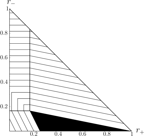
FIG. 6.: Contour lines over ${\cal W}^{P}$ for $E_{1}.$

FIG. 7.: Contour lines over ${\cal W}^{P}$ for $E_{S}.$

V Biseparable states: ${\cal B}_{1}$

In this section we are going to compute the set of biseparable states with respect to the partition $1|23.$ The technique is exactly the same as in the triseparable case: we first compute the set ${\cal B}_{\rm pure}$ of states of the form ${\bf P}(|\Psi\rangle\!\langle\Psi|)$ with $|\Psi\rangle\!\langle\Psi|$ biseparable, i.e., $\Psi=\psi_{1}\otimes\psi_{2,3}$. In a second step we get ${\cal B}_{1}$ as the convex hull of ${\cal B}_{\rm pure}$.

We are free to apply to our vector $\Psi$ a $U\otimes U\otimes U$ rotation without changing the projection. In this way we may choose $\psi_{1}=|1\rangle.$ Now the rotated state $\Psi^{\prime}$ is of the form $\Psi^{\prime}=\sum_{i,j}\psi_{ij}|1ij\rangle.$ The expectations of permutations of such a vector, like

$$\langle\Psi^{\prime}|V_{(12)}\Psi^{\prime}\rangle=\sum_{i,j,k,l}\overline{\psi_{ij}}\psi_{kl}\langle 1ij|k1l\rangle=\sum_{j}|\psi_{1j}|^{2}$$

then depend linearly on the following real parameters:

$$c_{0} = |\psi_{11}|^{2}$$ (34)

$$c_{1} = \sum_{j>1}|\psi_{1j}|^{2}$$ (35)

$$c_{2} = \sum_{i>1}|\psi_{i1}|^{2}$$ (36)

$$c_{3} = \sum_{i,j>1}\overline{\psi_{ij}}\psi_{ji}$$ (37)

$$c_{4}+ic_{5} = \sum_{j>1}\overline{\psi_{1j}}\psi_{j1}\;.$$ (38)

From this we obtain the following $r_{k}\mathpunct{:}$

$$r_{+}\! = \frac{1}{6}(1+5c_{0}+c_{1}+c_{2}+c_{3}+4c_{4})$$

$$r_{-}\! = \frac{1}{6}(1-c_{0}-c_{1}-c_{2}-c_{3})$$

$$r_{0} = \frac{2}{3}(1-c_{0}-c_{4})$$

$$r_{1} = \frac{1}{3}(-c_{1}-c_{2}+2c_{3}+4c_{4})$$

$$r_{2} = \frac{c_{1}-c_{2}}{\sqrt{3}}$$

$$r_{3} = \frac{2c_{5}}{\sqrt{3}}.$$

As in the tripartite case we need to determine the exact range of the parameters $c_{i}$. Let us assume $d>2$ for the moment. By the definitions of $c_{0},$ $c_{1}$ and $c_{2}$ we have

$$c_{0},c_{1},c_{2}\geq 0.$$ (39)

These parameters fix the weights of the blocks $(i=1,j=1)$, $(i=1,j>1)$, and $(i>1,j=1)$ in the normalization sum $\sum_{i,j=1}^{d}|\psi_{ij}|^{2}=1$. $c_{4}+ic_{5}$ can be read as the scalar product of two $(d-1)$-dimensional vectors $\varphi_{1}=(\psi_{12},\dots,\psi_{1d})$ and $\varphi_{2}=(\psi_{21},\dots,\psi_{d1})$ with norm squares $\|\varphi_{1}\|^{2}=c_{1}$ and $\|\varphi_{2}\|^{2}=c_{2}.$ By the Cauchy-Schwarz inequality we have:

$$c_{4}^{2}+c_{5}^{2}=|\langle\varphi_{1}|\varphi_{2}\rangle|^{2}\leq\|\varphi_{1}\|^{2}\|\varphi_{2}\|^{2}=c_{1}c_{2},$$ (40)

and any value of $c_{4}+ic_{5}$ consistent with this can actually occur.

We arrange the remaining $\psi_{ij}$ ($i,j>1$) into a $(d-1)^{2}$-dimensional vector $\widetilde{\Psi}=(\psi_{22},\dots,\psi_{2d},\psi_{32},\dots,\psi_{dd})$ with $\|\widetilde{\Psi}\|^{2}=1-c_{0}-c_{1}-c_{2}$. On this $(d-1)^{2}$-dimensional vector space, let $U$ denote the operator swapping $\psi_{ij}$ and $\psi_{ji}$. Then $c_{3}=\langle\widetilde{\Psi}|U\widetilde{\Psi}\rangle$ is the expectation of an hermitian operator with eigenvalues $\pm 1$. Hence

$$|c_{3}|\leq{\|\widetilde{\Psi}\|^{2}}=1-c_{0}-c_{1}-c_{2}\;,$$ (41)

and all $c_{3}\in{\mathbb{R}}$ satisfying this inequality can occur.

Together with the obvious modifications in the case $d=2$, when there is only one index $i>1$, we get the following Lemma:

Lemma 6

A tuple $(c_{0},c_{1},c_{2},c_{3},c_{4},c_{5})\in{\mathbb{R}}^{6}$ arises via equations (V) from a unit vector $\Psi$ in a $d^{2}$-dimensional Hilbert space, if and only if equations (39), (40) and (41) are satisfied, and, in the case $d=2,$ equality holds in (40) and (41).

Let $\Gamma$ denote the set of tuples $(c_{0},c_{1},c_{2},c_{3},c_{4},c_{5})$ satisfying these constraints. The $r_{k}$ depend linearly on the $c_{i}$, although the mapping is not one-to-one. Nevertheless any extreme point of ${\cal B}_{1}$ must be the image of an extreme point of the convex hull of $\Gamma$.

Hence we can proceed by first determine the extreme points of $\Gamma$. Since the positive variables $c_{0}$, $|c_{3}|$ and the sum $(c_{1}+c_{2})$ are only constrained by inequality (41), every point in $\Gamma$ is a convex combination of tuples in which only one of these is equal to $1$, and the other two vanish. This gives the extreme points

1. $c_{0}=1\Leftrightarrow\vec{r}=(1,0,0,0,0)\equiv B$

2. $c_{3}=+1\Leftrightarrow\vec{r}=(\frac{1}{3},0,\frac{2}{3},0,0)\equiv D$

3. $c_{3}=-1\Leftrightarrow\vec{r}=(0,\frac{1}{3},-\frac{2}{3},0,0)\equiv F$,

and furthermore some points with $(c_{1}+c_{2})=1$, $c_{0}=c_{3}=0$. Eliminating $c_{2}=1-c_{1}$ we can write inequality (40) as $c_{4}^{2}+c_{5}^{2}+(c_{1}-1/2)^{2}\leq 1/4$. This is a ball with extreme points parameterized by

$$c_{0} = 0,\quad c_{1}=\frac{1+\cos(\vartheta)}{2},\qquad c_{2}=\frac{1-\cos(\vartheta)}{2}$$

$$c_{3} = 0,\quad c_{4}=\frac{\sin(\vartheta)\cos(\varphi)}{2},\quad c_{5}=\frac{\sin(\vartheta)\sin(\varphi)}{2}$$

with $\varphi,\vartheta\in[0,2\pi].$ By mapping this description of $\Gamma$ to the $r_{k}$-parameterization we come to the following Theorem:

Theorem 7

The subset ${\cal B}_{1}\subset{\cal W}$ of biseparable states with respect to the partition $1|23$ has the following extreme points, described here in terms of the expectations $r_{k}=\mathop{\rm tr}\nolimits(\rho R_{k})$, $k=+,-,1,2,3$:

1. The sphere given by $\frac{1}{4}(3r_{1}+1)^{2}+3r_{2}^{2}+3r_{3}^{2}=1$ with $r_{-}=0$ and $r_{+}=(r_{1}+1)/{2}$ except for the point $(\frac{2}{3},0,\frac{1}{3},0,0)$, which is decomposable as $(\frac{2}{3},0,\frac{1}{3},0,0)=\frac{1}{2}(B+D)$

2. The point $F=(0,\frac{1}{3},-\frac{2}{3},0,0)$

3. The point $D=(\frac{1}{3},0,\frac{2}{3},0,0)$

4. The point $B=(1,0,0,0,0).$

A state $\rho\in{\cal W}$ is biseparable with respect to the partition $1|23$ if and only if it corresponds to the points F,B or D or the following inequalities are satisfied:

• $0\leq r_{-}<\frac{1}{3}$

• $-1<\frac{1+r_{1}-r_{-}-2r_{+}}{1-3r_{-}}<1$

• if $-1<\frac{1+r_{1}-r_{-}-2r_{+}}{1-3r_{-}}\leq 0$ then

  $$3r_{2}^{2}+3r_{3}^{2}+(1+2r_{1}+r_{-}-r_{+})^{2}\leq(2+r_{1}-4r_{-}-2r_{+})^{2}$$

• if $0\leq\frac{1+r_{1}-r_{-}-2r_{+}}{1-3r_{-}}<1$ then

  $$3r_{2}^{2}+3r_{3}^{2}+(1-3r_{-}-3r_{+})^{2}\leq(r_{1}+2r_{-}-2r_{+})^{2}.$$

We omit here again the computation of these inequalities from the known extreme points. They can be obtained by projecting from the three points $F,B$ and $D$ onto the sphere of extremal points.

The projection of the set ${\cal B}_{1}$ onto ${\cal W}^{P}$ comes to be equal to the projection of the set of pure ${\cal B}_{1}$-states and was already shown in Figure 2 together with the section ${\cal B}_{1}\cap{\cal W}^{P}.$ To compare ${\cal B}_{1}$ with ${\cal T}$ we plot again the section with $r_{+}=0.27$ and $r_{-}=0.1$ (Figure 8).

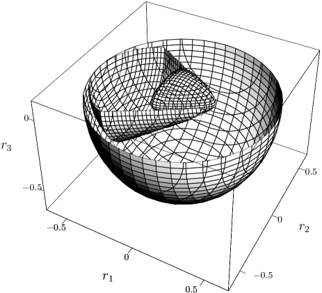
FIG. 8.: Plot of the set ${\cal B}_{1}$ for $r_{+}=0.27$ and $r_{-}=0.1$ embedded in the respective Bloch sphere together with ${\cal T}.$

To make the inclusion ${\cal T}\subsetneq({\cal B}_{1}\cap{\cal B}_{2}\cap{\cal B}_{3})$ we mentioned in the introduction more evident we can now compute the sets ${\cal B}_{2}$ and ${\cal B}_{3}$ to build their intersection with ${\cal B}_{1}.$ Due to the permutation symmetry of the three subsystems we can rotate ${\cal B}_{1}$ by $\pm\frac{2\pi}{3}$ in the $r_{1}$-$r_{2}$-plane instead. This leads to Figure 9:

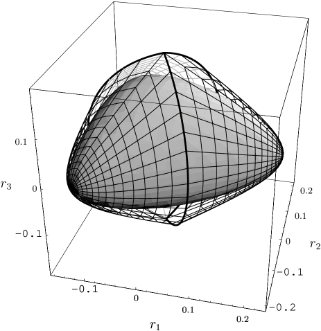
FIG. 9.: The intersection ${\cal B}_{1}\cap{\cal B}_{2}\cap{\cal B}_{3}$ is shown as mesh on a transparent surface allowing the set ${\cal T}$ to be seen. This plot is again computed for the section $r_{+}=0.27$ and $r_{-}=0.1.$ The thick lines indicate the intersection of two of the biseparable sets.

VI Positive partial transposes: ${\cal P}_{1}$

One of the interesting aspects in the theory of bipartite entanglement to emerge in recent years was the consideration of the partial transpose of the density matrix, and in particular the positivity of the partial transpose. First, this positivity served as a necessary condition for separability, which is even sufficient in $2\otimes 2$ and $2\otimes 3$ dimensions (the Peres criterion [5]). Moreover, it is a necessary condition for undistillability, and here it comes much closer to sufficiency even in general situations. Both aspects play a role in the analysis of tripartite states. We will therefore describe in this section the subset ${\cal P}_{1}\subset{\cal W}$ of states with positive $1$-transpose.

Since the dimensions for this bipartite system are $d\otimes d^{2}$, positive partial transpose does not automatically imply biseparability, i.e., the inclusion ${\cal B}_{1}\subset{\cal P}_{1}$ may be strict. However, since we are considering a special class of states it is also possible that in this class equality holds. This does happen, for example, for the bipartite Werner states [11]. In the tripartite case we will see that ${\cal B}_{1}={\cal P}_{1}$ for $d=2$, but not for higher dimensions, although the two sets come to be remarkably close (see Figure 13). However, the exact description of ${\cal P}_{1}$ is also important for distillation questions.

The partial transpose $A\mapsto A^{T_{1}}$ of operators on ${\cal H}_{1}\otimes{\cal H}_{2}$ was defined in Equation (2). In a tripartite system we take this operation to refer to the first of the three tensor factors, and write $\rho\in{\cal P}_{1}$ if $\rho^{T_{1}}\geq 0$.

A The algebra of partial transposes

When $\rho$ is a linear combination of permutation operators as in Lemma 1, the partial transpose

$$\rho^{T_{1}}=\sum_{\pi}{\mu}_{\pi}V_{\pi}^{T_{1}}$$

is likewise a linear combination of the six operators $V_{\pi}^{T_{1}}$, and we have to decide for which coefficients ${\mu}_{\pi}$ such an operator is positive. Since partial transposition is not a homomorphism, it would appear that the linear combinations of the $V_{\pi}^{T_{1}}$ can be a fairly arbitrary space of operators, and deciding positivity could be quite difficult. However, it turns out that these linear combinations do form an algebra, so after the introduction of the right basis deciding positivity is just as easy as determining the state space in Lemma 2.

The abstract reason for this “happy coincidence” is that the operators $V_{\pi}^{T_{1}}$ span the set of fixed points of an averaging operation in much the same way as the permutations span the set of fixed points of ${\bf P}$. The corresponding averaging operator is

$$\widetilde{{\bf P}}\rho=\int\!dU\ (\overline{U}\otimes U\otimes U)\rho\,(\overline{U}\otimes U\otimes U)^{*}.$$ (42)

Its range consists of all operators commuting with all unitaries of the form $\overline{U}\otimes U\otimes U$, hence is an algebra. The following Lemma describes the relation between $\widetilde{{\bf P}}$ and ${\bf P}$:

Lemma 8

Let $A$ be any hermitian operator, then

1. ${\bf P}A=A\Leftrightarrow\widetilde{{\bf P}}A^{T_{1}}=A^{T_{1}}$

2. $\left(\widetilde{{\bf P}}A\right)^{T_{1}}={\bf P}\left(A^{T_{1}}\right).$

Proof: For any hermitian operator $A$ one has:

$$\widetilde{{\bf P}}A=A \Leftrightarrow \left[\overline{U}\otimes U\otimes U,A\right]_{-}={\bf 0}$$

$$\Leftrightarrow \left[U\otimes U\otimes U,A^{T_{1}}\right]_{-}={\bf 0}$$

$$\Leftrightarrow {\bf P}A^{T_{1}}=A^{T_{1}}.$$

Furthermore we can compute directly:

$${\bf P}A^{T_{1}} = \int\!dU\ (U\otimes U\otimes U)A^{T_{1}}\,(U\otimes U\otimes U)^{*}$$

$$= \int\!dU\ \bigl{(}(\overline{U}\otimes U\otimes U)A\,(\overline{U}\otimes U\otimes U)^{*}\bigr{)}^{T_{1}}$$

$$= \bigl{(}\widetilde{{\bf P}}A\bigr{)}^{T_{1}}.$$

        

For deciding positivity of partial transposes we need a concrete form of the algebra spanned by the partial transposes of the permutation operators. For example, we get

$$V_{(12)}^{T_{1}} = \sum_{ijk}\Bigl{(}|ijk\rangle\!\langle jik|\Bigr{)}^{T_{1}}=\sum_{ijk}|jjk\rangle\!\langle iik|$$

$$= (|\Phi\rangle\!\langle\Phi|)\otimes{\openone},$$

where $\Phi=\sum_{i}|ii\rangle$ is a maximally entangled vector of norm $d$. The partial transposes of the other permutations are computed similarly. We can express all of them in terms of the first two:

$$X=V_{(12)}^{T_{1}}\qquad{\rm and}\qquad V=V_{(23)}^{T_{1}}=V_{(23)}$$ (43)

as

$${\openone}^{T_{1}}={\openone},\quad V_{(13)}^{T_{1}}=VXV,\quad V_{(123)}^{T_{1}}=XV,\quad V_{(321)}^{T_{1}}=VX.$$

Then these operators satisfy the relations $X^{*}=X,$ and $V^{*}=V$, and

$$X^{2}=dX\ ,\qquad V^{2}={\openone}\ ,\qquad XVX=X.$$ (44)

Due to these relations the set of linear combinations of the six operators $\{{\openone},X,VXV,V,XV,VX\}$ is closed under adjoints and products. Positivity of such linear combinations, and hence the positivity of all partial transposes of operators in ${\cal W}$ can therefore be decided by studying the abstract algebra generated by two hermitian elements $X$ and $V$ satisfying (44). As a six dimensional non-commutative C*-algebra it is isomorphic to the algebra generated by the permutations, i.e., a sum of two one dimensional and a two dimensional matrix algebra. But of course, the partial transpose operation mapping one into the other is not a homomorphism.

From these considerations it is clear that all we have to do now is to find a basis of the algebra generated by $X$ and $V$ analogous to the basis (1). This sort of computation can be quite painful, so we recommend the use of a symbolic algebra package. The result is

$$S_{+} = \frac{{\openone}+V}{2}\Bigl{(}{\openone}-\frac{2X}{d+1}\Bigr{)}\frac{{\openone}+V}{2}$$ (46)

$$S_{-} = \frac{{\openone}-V}{2}\Bigl{(}{\openone}-\frac{2X}{d-1}\Bigr{)}\frac{{\openone}-V}{2}$$ (47)

$$S_{0} = \frac{1}{d^{2}-1}\ \Bigl{(}d(X+VXV)-(XV+VX)\Bigr{)}$$ (48)

$$S_{1} = \frac{1}{d^{2}-1}\ \Bigl{(}d(XV+VX)-(X+VXV)\Bigr{)}$$ (49)

$$S_{2} = \frac{1}{\sqrt{d^{2}-1}}\ \Bigl{(}X-VXV\Bigr{)}$$ (50)

$$S_{3} = \frac{i}{\sqrt{d^{2}-1}}\ \Bigl{(}XV-VX\Bigr{)}.$$ (51)

These operators satisfy exactly the same relations as the $R_{k}$ from (1) and we will denote the corresponding expectation values by $s_{k}(\rho):=\mathop{\rm tr}\nolimits(\rho S_{k}).$ The two projections $S_{\pm}$ correspond to the two one-dimensional representations of the algebra, i.e., to the two realizations of the relations by c-numbers, namely $X=0,V=1$ and $X=0,V=-1$.

B The $V_{(23)}$-invariant case

The simplest case is the $V_{(23)}$-invariant subset of ${\cal W}$ as it is a three dimensional object. In fact the $V_{(23)}$-invariance implies the conditions $\mathop{\rm tr}\nolimits(\rho V_{(23)})\!=1,$ $\mathop{\rm tr}\nolimits(\rho V_{(12)})\!=\mathop{\rm tr}\nolimits(\rho V_{(31)})$ and $\mathop{\rm tr}\nolimits(\rho V_{(123)})\!=\mathop{\rm tr}\nolimits(\rho V_{(321)}).$ Therefore we have $r_{2}=r_{3}=0.$ In the same way we obtain for a $V_{(23)}$-invariant state $\rho\in{\cal W}^{T_{1}}$ the conditions $s_{2}=0$ and $s_{3}=0.$ Positivity of a $V_{(23)}$-invariant state in ${\cal W}$ requires now $r_{+}\geq 0,$ $r_{-}\geq 0$ and $|r_{1}|\leq r_{0}=1-r_{+}-r_{-}$ (cf. (13)) giving raise to a tetrahedron bounded by the hyperplanes

$$(h_{1})\ r_{+}\!=0,\qquad(h_{2})\ r_{-}=0,\qquad(h_{3})\ r_{1}=1-r_{+}-r_{-}$$

$$(h_{4})\ r_{1}=r_{+}+r_{-}-1$$

and having the extreme points $P_{1}=(0,0,1),$ $P_{2}=(0,0,-1),$ $P_{3}=(0,1,0),$ and $P_{4}=(1,0,0).$ The same computation can be done on the partially transposed side leading to the tetrahedron confined by the hyperplanes

$$(h^{\prime}_{1})\ s_{+}\!=0,\qquad(h^{\prime}_{2})\ s_{-}=0,\qquad(h^{\prime}_{3})\ s_{1}=1-s_{+}-s_{-}$$

$$(h^{\prime}_{4})\ s_{1}=s_{+}+s_{-}-1.$$

Using Lemma 8 we can express the $s_{k}$ by the $r_{k}$ of the corresponding ${\cal W}$-state. Multiplying by positive constants one gets an easier description of these hyperplanes:

$$(h^{\prime}_{1})\ 2(1+r_{1}-r_{-}-2r_{+})+d(1+r_{1}-r_{-}+r_{+})=0$$

$$(h^{\prime}_{2})\ 2(-1+r_{1}+2r_{-}+r_{+})+d(1-r_{1}+r_{-}-r_{+})=0$$

$$(h^{\prime}_{3})\ 1-r_{1}-5r_{-}-r_{+}=0$$

$$(h^{\prime}_{4})\ 1+r_{1}-r_{-}-5r_{+}=0.$$

Its four extremal points are now $Q_{1}=(\frac{2+d}{3},0,\frac{1-d}{3}),$ $Q_{2}=(0,\frac{2-d}{3},-\frac{1+d}{3}),$ $Q_{3}=(0,\frac{1}{3},-\frac{2}{3})$ and $Q_{4}=(\frac{1}{3},0,\frac{2}{3}).$ Of course, these point have no reason to correspond to positive states, and indeed only $Q_{3}$ and $Q_{4}$ lie inside the state space, where $Q_{1}$ and $Q_{4}$ are outside the state space for all $d$.

As we are looking for those $V_{(23)}$-invariant ${\cal W}$-states that have positive partial transpose, i.e. that lie in ${\cal P}_{A},$ we have now to look at the intersection of these two tetrahedra. The resulting object is again a tetrahedron as one can see in Figure 10. This is due to the fact, that the extremal points $P_{i}$ and $Q_{i}$ ($i=1,2,3,4$) lie on just two straight lines, namely $\overline{P_{1}Q_{4}P_{4}Q_{1}}$ and $\overline{Q_{2}P_{2}Q_{3}P_{3}}.$ The intersection of the two tetrahedra is hence again a tetrahedron, spanned by the extremal points $P_{2}$, $P_{4}$, $Q_{3}$ and $Q_{4}$ (called $E$, $B$, $F$, and $D$ in Sections II B and V), and is thus dimension independent. But it is easily verified from Theorem 7 that these four points are precisely the extreme points of the $V_{(23)}$-invariant part of ${\cal B}_{1}$. Since ${\cal B}_{1}\subset{\cal P}_{1}$, we have shown the following:

Lemma 9

A $V_{(23)}$-invariant ${\cal W}$-state has a positive partial transpose if and only if it is biseparable.

FIG. 10.: The two positivity tetrahedra bounded by the $h_{i}$ (dotted) and the $h^{\prime}_{i}$ (dashed) and the intersection tetrahedron (solid lines) for $d=3.$

As we will see in the next subsection, the assumption of $V_{(23)}$-invariance is essential, i.e., the conclusion does not hold for general ${\cal W}$-states.

In order to see how $V_{(23)}$-invariance helps, we conclude this subsection with a direct proof of the above Lemma for $d=2$. If $\rho$ is a $V_{(23)}$-invariant ${\cal W}$-state, then we can decompose it into the following sum

$$\rho\! = \!\frac{1}{4}\bigl{(}{\openone}+V_{(23)}\bigr{)}\rho\bigl{(}{\openone}+V_{(23)}\bigr{)}\!+\frac{1}{4}\bigl{(}{\openone}-V_{(23)}\bigr{)}\rho\bigl{(}{\openone}-V_{(23)}\bigr{)}$$

$$=\mathpunct{:} \rho^{+}+\rho^{-}.$$

It is now clear that $\rho$ has a positive partial transpose iff both $\rho^{+}$ and $\rho^{-}$ each have a positive partial transpose. $\rho^{+}$ denotes the $V_{(23)}$-symmetric part of $\rho,$ $\rho^{-}$ the antisymmetric part. Thus we know that $\rho^{+}$ is a $2\times 3$ density operator and $\rho^{-}$ a $2\times 1.$ For these systems the Peres criterion holds strictly [12], i.e. states have a positive partial transpose iff they are separable or in our case biseparable over the $1|23$ split. Biseparability of $\rho^{+}$ and $\rho^{-}$ is equivalent to the biseparability of $\rho$, which proves the lemma.         

C The general case

The positivity conditions for arbitrary linear combinations of the operators $S_{k}$ give the following result:

Lemma 10

Let $\rho\in{\cal W}$ be a density operator with expectations $r_{k}=\mathop{\rm tr}\nolimits(\rho R_{k})$, $k=+,-,1,2,3$. Then the partial transpose of $\rho$ with respect to the first tensor factor is positive,i.e. $\rho\in{\cal P}_{1},$ if and only if

$$0 \leq r_{-}$$ (53)

$$0 \leq r_{1}-r_{+}-r_{-}+1$$ (54)

$$0 \leq 1-r_{1}-5r_{-}-r_{+}$$ (55)

$$0 \leq -1-r_{1}+r_{-}+5r_{+}$$ (56)

$$r_{2}^{2}+r_{3}^{2} \leq R_{1}$$ (57)

$$r_{2}^{2}+r_{3}^{2} \leq R_{2}$$ (58)

where

$$R_{1} := (1-r_{1}-5r_{-}-r_{+})(-1-r_{1}+r_{-}+5r_{+})/3$$

$$R_{2} := (1-r_{1}-r_{-}-r_{+})(1+r_{1}-r_{-}-r_{+}).$$

Proof: Recall that averaging with respect to $V_{(23)}$ projects ${\cal P}_{1}$ to the section of ${\cal P}_{1}$ with $r_{2}=r_{3}$. Therefore, the inequalities describing the tetrahedron discussed in the last subsection are optimal. These are the first four inequalities. We therefore only have to describe the admissible set of $(r_{2},r_{3})$, given $(r_{+},r_{-},r_{1})$. There are two conditions to consider, one from the positivity of $\rho$, and one from the positivity of $\rho^{T_{1}}$. As shown in the first subsection, both these requirements have a very similar form, namely the positivity of an element in an abstract algebra with two one-dimensional summands and one summand isomorphic to the $2\times 2$-matrices. Now in both cases $(r_{+},r_{-},r_{1})$ are readily seen to fix the weights of the one-dimensional parts, as well as the trace and the expectation of the first Pauli matrix for the $2\times 2$-part. This leaves a condition of the form $r_{2}^{2}+r_{3}^{2}\leq R$ in both cases. The two conditions are given in the Lemma, where $R_{2}=(1-r_{+}-r_{-})^{2}-r_{1}^{2}$ expresses the requirement $\rho\geq 0$. The condition (57) is obtained from $\rho^{T_{1}}\geq 0$ by expressing $\rho^{T_{1}}$ in the basis $S_{k}$, and applying the same criterion to the expectations $s_{k}$.         

According to this Lemma the set ${\cal P}_{1}$ can be visualized as follows: firstly, one has to fix a point $(r_{+},r_{-})$ in the permutation invariant triangle (Figure 2). The possible choices of $(r_{1},r_{2},r_{3})$ can then be seen from Figure 8. Apart from the heart shaped tripartite set in the center this Figure contains three quadratic surfaces: the Bloch sphere, and the two surfaces bounding ${\cal B}_{1}$. Comparing condition (d) of Theorem 7 and the expression for $R_{1}$ given in the above Lemma, we find that both constraints are given by the same hyperboloid, the one wrapped around the tripartite set in Figure 8. Hence in that Figure we can readily find ${\cal P}_{1}$ by extending this hyperboloid all the way to the Bloch sphere, and taking the intersection. This is shown in Figure 11, in the section $r_{3}=0$.

FIG. 11.: Plot of the Bloch sphere, ${\cal T},$ ${\cal B}_{1}$ and ${\cal P}_{1}$ for $r_{+}=0.27,$ $r_{-}=0.1$ and $r_{3}=0.$

Figure 11 shows the generic situation with $r_{-}\neq 0$. When $r_{-}=0$, in particular for systems of three qubits, the boundary ellipsoid of ${\cal B}_{1}$, described by condition (c) of Theorem 7, coalesces with the Bloch sphere. This leads to another instance where the Peres-Horodecki criterion for separability holds:

Corollary 11

The intersections of ${\cal B}_{1}$ and ${\cal P}_{1}$ with the plane $r_{-}=0$ coincide. In particular, for $3$-qubit ${\cal W}$-states, biseparability is equivalent to the positivity of the partial transpose.

We conclude this section by the explicit determination of the extreme points of ${\cal P}_{1}$. From Figure 11 it might appear that all points on the quadratic surfaces bounding ${\cal P}_{1}$ might be extremal. But this is misleading, because we also have to take into account the possibility of decompositions with different values of $(r_{+},r_{-})$. In fact, for the inequalities arising from $\rho\geq 0$ it is evident that generically such decompositions are possible: given any $(r_{+},r_{-},r_{1},r_{2},r_{3})$, which lies on the Bloch sphere in Figure 11, we can just change the weights of the three blocks in the block decomposition of $\rho$ according to $(\lambda_{+}r_{+},\lambda_{-}r_{-},\lambda_{0}r_{1},\lambda_{0}r_{2},\lambda_{0}r_{3}))$, as long as the $\lambda_{\alpha}$ are positive, and the normalization $\lambda_{+}r_{+}+\lambda_{-}r_{-}+\lambda_{0}(1-r_{+}-r_{-})=1$ is respected. This leaves a two dimensional affine manifold through $(r_{+},r_{-},r_{1},r_{2},r_{3})$. Hence, unless other conditions constraining ${\cal P}_{1}$ prevent the indicated decompositions no such point will be extremal. Of course, the second constraint (57) has the same structure, because the algebra of partial transposes is isomorphic to the algebra generated by the states. Hence in Figure 11 only the points in the intersection of the hyperboloid and the Bloch sphere remain as candidates for extreme points. This is analogous to the extreme points of ${\cal B}_{1}$, which also consist of the intersection of two quadratic surfaces in Figure 11. For ${\cal P}_{1}$ we get

Theorem 12

The subset ${\cal P}_{1}\subset{\cal W}$ of ${\cal W}$-states with positive 1-transpose has the following extreme points, described here in terms of the expectations $r_{k}=\mathop{\rm tr}\nolimits(\rho R_{k})$, $k=+,-,1,2,3$:

1. The points $P_{2},$ $Q_{3},$ $P_{4},$ and $Q_{4}$, which also span the $V_{(23)}$-invariant part of ${\cal P}_{1}$.

2. the remaining extreme points of ${\cal B}_{1}$, which form a sphere in the $r_{-}=0$ plane (cf. Theorem 7).

3. The points for which $(r_{+},r_{-},r_{1},0,0)$ lie in the interior of the $V_{(23)}$-invariant tetrahedron, and for which inequalities (57) and (58) are both satisfied with equality.

Proof: Let us first discuss the periphery of the tetrahedron. Every face of the tetrahedron corresponds to a face of ${\cal P}_{1}$, namely the face of points projecting to it upon $V_{(23)}$-averaging. In Lemma 10 this corresponds to the subsets for which one of the linear inequalities (10a) to (10d) is equality. We will show first that each of these faces is actually contained in ${\cal B}_{1}$. Indeed, when (10b), (10c) or (10d) are equalities, one of the factors in $R_{1}$ or $R_{2}$ vanishes, forcing $r_{2}=r_{3}=0$, reducing our claim to Lemma 9. When (10a) is equality, i.e., $r_{-}=0$, the claim is contained in Corollary 11.

Now a point of ${\cal P}_{1}$ contained in one of these faces can only have decompositions in the same face, hence in ${\cal B}_{1}$, hence for such a point extremality in ${\cal P}_{1}$ and extremality in ${\cal B}_{1}$ are equivalent.

It remains to show item 3 of the Theorem, i.e., to characterize the extreme points of ${\cal P}_{1}$, whose $V_{(23)}$-averages fall in the interior of the tetrahedron. From the arguments preceding the Theorem it is clear that points for which only one of the inequalities (57) and (58) are equalities cannot be extremal, since the surfaces defined by these equations contain straight lines. Therefore, the condition stated in the Theorem is necessary for a point to be extremal. It remains to show that none of the points with $R_{1}=R_{2}$ can be decomposed in a proper convex combination.

Let us denote by $M_{1}$ (resp. $M_{2}$) the set of those points in the interior of the tetrahedron such that $R_{1}\leq R_{2}$ (resp. $R_{2}\leq R_{1}$). The intersection $M_{*}=M_{1}\cap M_{2}$ of these sets is described by the condition $R_{1}=R_{2}$, or explicitly

$$r_{1}^{2}+3r_{-}+r_{1}r_{-}-2r_{-}^{2}+3r_{+}-r_{1}r_{+}-8r_{-}r_{+}-2r_{+}^{2}\!=\!1.$$ (59)

This is a one-sheet hyperboloid, generated by two sets of straight lines shown in Figure 12. Consider a line segment

$$u\mapsto(\hat{r}_{+},\hat{r}_{-},\hat{r}_{1})+u(t_{+},t_{-},t_{1})$$ (60)

through one of the points $\hat{p}=(\hat{r}_{+},\hat{r}_{-},\hat{r}_{1})\in M_{*}$ of the hyperboloid. Consider the radius functions $\sqrt{R_{i}}$, evaluated as a function of the parameter $u$. If such a function is affine (has vanishing second derivative) we can set $(r_{1}(u),r_{2}(u))=(\cos\alpha,\sin\alpha)\sqrt{R_{i}}$ with arbitrary $\alpha$, to get a straight line in the corresponding hypersurface in $5$ dimensions. We then call $(t_{+},t_{-},t_{1})$ an affine direction for $R_{i}$. Along other directions, $R_{i}$ is strictly concave, so no decomposition along the segment (60) is possible. For both radius functions, the set of affine directions is a two-dimensional plane, and thus best described by its normal vector. That is, $\vec{t}=(t_{+},t_{-},t_{1})$ is an affine direction for $R_{i}$ if $\vec{t}\cdot\vec{A}_{i}=0$, where

$$\vec{A}_{1}=\left(\begin{array}[]{c}2-3\hat{r}_{1}-12\hat{r}_{-}\\ -2-3\hat{r}_{1}+12\hat{r}_{+}\\ -1+3\hat{r}_{-}+3\hat{r}_{+}\end{array}\right)\quad\vec{A}_{2}=\left(\begin{array}[]{c}-\hat{r}_{1}\\ -\hat{r}_{1}\\ -1+\hat{r}_{-}+\hat{r}_{+}\end{array}\right).$$ (61)

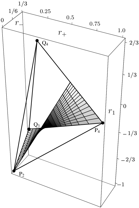
FIG. 12.: Section of the intersecting tetrahedron with the separating one-leaf hyperboloid.

Assuming that a convex decomposition along (60) is possible, we thus arrive at a threefold case distinction:

• The line segment lies entirely in $M_{1}$.
  Then it must be tangent to the hyperboloid $M_{*}$, and also an affine direction for $R_{1}$. The vector $\vec{t}$ is uniquely determined up to a factor by these conditions. However, that does not mean that the corresponding line segment lies in $M_{1}$, and, in fact, one can show that it never does. Hence this case is ruled out.

• The line segment lies entirely in $M_{2}$.
  This is ruled out analogously.

• The line segment crosses from $M_{1}$ into $M_{2}$.
  Then $\vec{t}$ must be affine for both radius functions. Again, this determines $\vec{t}$ to within a factor. But for a proper decomposition we must have also that the slopes of $\sqrt{R_{1}}$ and $\sqrt{R_{2}}$ match at $u=0$. One can show that this never happens inside the tetrahedron we discuss, so this case is also ruled out.

We conclude that no point on $M_{*}$ allows a convex decomposition inside ${\cal P}_{1}$, and the theorem is proved.

Analysis of $\widetilde{{\bf P}}$

In this appendix we give a characterization of the separability classes ($\widetilde{{\cal T}},$ $\widetilde{{\cal B}}_{1},$ and $\widetilde{{\cal P}}_{1}$) of $\widetilde{{\bf P}}$ showing that they can be deduced from those of ${\bf P}$ without any computation.

The intimate relation between the two twirls emerged already in Lemma 8 where we stated the existence of an isomorphism between the two algebras spanning the eigenspaces of ${\bf P}$ and $\widetilde{{\bf P}}$. This isomorphism establishes an affine mapping $\iota$ between the two eigenspaces that we used to compute ${\cal P}_{1}.$ Due to the inclusion ${\cal T}\subsetneq{\cal B}_{1}\subsetneq{\cal P}_{1}$ it is clear that the same mapping transports the sets ${\cal T}$ and ${\cal B}_{1}$ to their counterparts $\widetilde{{\cal T}}$ and $\widetilde{{\cal B}}_{1}.$ The mapping $\iota$ can be computed by fixing the ordering $\{{\openone},X,V,VXV,XV,VX\}$ for the second algebra and concatenating the transformations 1 and 8 getting

$$\vec{s}=\iota\cdot{\vec{r}}$$

with

$$\iota=\left(\begin{array}[]{cccccc}\frac{d-1}{d+1}&0&\frac{d+2}{2d+2}&\frac{d+2}{2d+2}&0&0\\ 0&\frac{d+1}{d-1}&\frac{d-2}{2d-2}&\frac{2-d}{2d-2}&0&0\\ \frac{2}{d+1}&-\frac{2}{d-1}&\frac{1}{d^{2}-1}&-\frac{d}{d^{2}-1}&0&0\\ \frac{2}{d+1}&\frac{2}{d-1}&-\frac{d}{d^{2}-1}&\frac{1}{d^{2}-1}&0&0\\ 0&0&0&0&\frac{\sqrt{3}}{\sqrt{d^{2}-1}}&0\\ 0&0&0&0&0&\frac{\sqrt{3}}{\sqrt{d^{2}-1}}\end{array}\right).$$

With this mapping we can compute directly the $\widetilde{{\bf P}}$-projection of the states A to G:

$$A: |123\rangle\longrightarrow(1/2,1/2,0,0,0)$$

$$B: |111\rangle\longrightarrow\left(\frac{d-1}{d+1},0,\frac{2}{d+1},0,0\right)$$

$$C: (|111\rangle-\sqrt{3}|112\rangle+\sqrt{3}|121\rangle-3|122\rangle)/4$$

$$\qquad\qquad\qquad\longrightarrow\left(\frac{4+5d}{8+8d},\frac{3d-6}{8d-8},\frac{d+2}{4-4d^{2}},0,0\right)$$

$$D: |122\rangle\longrightarrow(1,0,0,0,0)$$

$$E: (|112\rangle-|121\rangle)/\sqrt{2}\longrightarrow\left(0,\frac{d-2}{d-1},\frac{1}{1-d},0,0\right)$$

$$F: (|123\rangle-|132\rangle)/\sqrt{2}\longrightarrow(0,1,0,0,0)$$

$$G: (|112\rangle-|121\rangle-\sqrt{3}|122\rangle)/\sqrt{5}$$

$$\qquad\qquad\qquad\longrightarrow\left(\frac{3}{5},\frac{2d-4}{5d-5},\frac{2}{5-5d},0,0\right)$$

Applying the transformation to the extremal points and inequalities of Theorems 5, 7 and 12 yields then a characterization of $\widetilde{{\cal T}},$ $\widetilde{{\cal B}}_{1}$ and $\widetilde{{\cal P}}_{1}.$

We omit here the results of these transformations and give the picture corresponding to Fig.2:

FIG. 13.: Sections and projections of $\widetilde{{\cal T}}$ and ${\widetilde{{\cal B}}_{1}}$ with/onto the $s_{+}$-$s_{-}$-plane for $d=3.$ Black: section with $\widetilde{{\cal T}},$ dark grey: projection of $\widetilde{{\cal T}},$ light grey: section with $\widetilde{{\cal B}}_{1}.$

In contrast to what can be seen in Fig.2 the projection of $\widetilde{{\cal T}}$ onto the $s_{+}$-$s_{-}$-plane differs from its section with it as one can see in Fig.14:

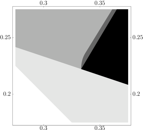
FIG. 14.: Zoomed region of Fig.11.

REFERENCES

- [1] R. F. Werner, Phys. Rev. A 40, 4277 (1989).
- [2] S. Popescu, Phys. Rev. Lett. 72, 797 (1994).
- [3] C. H. Bennett, D. P. DiVincenzo, J. A. Smolin, and W. K. Wootters, Phys. Rev. A 54, 3824 (1996).
- [4] W. Dür, J. I. Cirac, and R. Tarrach, Phys. Rev. Lett. 83 3562 (1999).
- [5] A. Peres, Phys. Rev. Lett. 77 1413 (1996).
- [6] C. H. Bennett et al., Phys. Rev. Lett. 82 5385 (1999).
- [7] H. Weyl, The Classical Groups, (Princeton University, 1946).
- [8] A. Elby and J. Bub, Phys. Rev. A 49 4213 (1994).
- [9] M. A. Nielsen, Phys. Rev. Lett. 82 436 (1999).
- [10] M. Ohya and D. Petz, Quantum entropy and its use, (Springer, 1993).
- [11] M. Horodecki and P. Horodecki, Phys. Rev. A 59, 4206 (1999).
- [12] M. Horodecki, P. Horodecki and R. Horodecki, Phys. Lett. A 223 1 (1996).