Entanglement Measures under Symmetry

Abstract

We show how to simplify the computation of the entanglement of formation and the relative entropy of entanglement for states, which are invariant under a group of local symmetries. For several examples of groups we characterize the state spaces, which are invariant under these groups. For specific examples we calculate the entanglement measures. In particular, we derive an explicit formula for the entanglement of formation for $U\otimes U$-invariant states, and we find a counterexample to the additivity conjecture for the relative entropy of entanglement.

I Introduction

One of the reasons the general theory of entanglement has proved to be so difficult is the rapid growth of dimension of the state spaces. For bipartite entanglement between $d_{1}$- and $d_{2}$-dimensional Hilbert spaces, entanglement is a geometric structure in the $(d_{1}^{2}d_{2}^{2}-1)$-dimensional state space. Hence even in the simplest non-trivial case ($d_{1}=d_{2}=2$; 15 dimensions) naive geometric intuitions can be misleading. On the other hand, the rapid growth of dimensions is partly responsible for the potential of quantum computing. Hence exploring this complexity is an important challenge for quantum information theory.

Model studies have been an important tool for developing and testing new concepts and relations in entanglement theory, both qualitative and quantitative. In this paper we explore a method for arriving at a large class of models, which are at the same simple, and yet show some of the interesting features of the full structure.

The basic idea, namely looking at sets of states which are invariant under a group of local unitaries is not new, and goes back to the first studies of entanglement [1, 2] in the modern sense. Two classes, in particular, have been considered frequently: the so-called Werner states (after[1]), which are invariant under all unitaries of the form $U\otimes U$, and the so-called isotropic states [3], which are invariant under all $U\otimes\overline{U}$, where $\overline{U}$ is the complex conjugate of $U$ in some basis. Symmetry has also been used in this way to study tripartite entanglement [4],[5]. A recent paper of Rains [6] discusses distillible entanglement under symmetry, so we have eliminated the pertinent remarks from this paper.

Several of the ingredients of our general theory, for example the role of the twirl projection and the commutant, have been noted in these special cases and can be considered to be well-known. The computation of the relative entropy of entanglement [7] was known [8] for Werner states. The first study in which symmetry is exploited to compute the entanglement of formation [9] beyond the Wootters formula [10] is [12], where the case of isotropic states is investigated. Our theory of entanglement of formation can be viewed as an abstract version of arguments from that paper.

What is new in the present paper is firstly the generality. We regard our theory as a toolkit for constructing examples adapted to specific problems, and we have tried to present it in a self-contained way facilitating such applications. Exploring all the possibilities would have been too much for a single paper but, of course, we also have some new results in specific examples.

Our most striking specific result is perhaps a counterexample to the conjecture that the relative entropy of formation should be additive. The evidence in favor of this conjecture had been partly numerical, but it was perhaps clear that a random search for counterexamples was not very strong evidence to begin with: the relative entropy of entanglement is defined by a variational formula in a very high dimensional space, whose solution is itself not easy to do reliably. In addition, the additivity conjecture is true on a large set in the state space, so unless one has a specific idea where to look, a random search may well produce misleading evidence. The second strong point in favor of the additivity conjecture had been a Theorem by Rains (Theorems 4 and 5 in [13]) implying a host of non-trivial additivity statements. However, our counterexample satisfies the assumptions of the Rains’ Theorem, so that Theorem is, unfortunately, false.

Further specific results in our paper are the formulas for entanglement of formation and relative entropy of entanglement for Werner states.

The paper is organized as follows: In Section II we review the essential techniques for the investigation of symmetric states and describe how the partial transposition fit in this context. Section II.D presents a zoo of different symmetry groups. Some of these are used later, others are only presented as briefly, to illustrate special properties possible in this setup. We hope that this list will prove useful for finding the right tradeoff between high symmetry, making an example manageable, and richness of the symmetric state space, which may be needed to see the phenonmenon under investigation. In Section III we briefly recapitulate the definitions of the entanglement of formation and the relative entropy of entanglement and the additivity problem. In Section IV we turn to the entanglement of formation. We show first how the computation may be simplified using local symmetry. These ideas are then applied to the basic symmetry groups $UU$ and $U\overline{U}$, arriving at an explicit formula in both cases (the results for $U\overline{U}$ are merely cited here for completeness from work of the first author with B. Terhal[12]). For the group $OO$ of orthogonal symmetries, which unifies and extends these two examples, we find formulas in large sections of the state space. Section V deals with the relative entropy of entanglement. Again we begin by showing how the computation is simplified under symmetry. We then present the counterexample to additivity mentioned in the introduction. Some possible extensions are mentioned in the concluding remarks.

II Symmetries and Partial Transposes

From the beginning of the theory of entanglement the study of special subclasses of symmetric states has played an important role. In this section we give a unified treatment of the mathematical structure underlying all these studies. For simplicity we restrict attention to the bipartite finite dimensional case, although some of the generalizations to more than two subsystems [4] and infinite dimension are straightforward. So throughout we will consider a composite quantum system with Hilbert space ${\cal H}={\cal H}_{1}\otimes{\cal H}_{2}$, with $\dim{\cal H}_{i}=d_{i}<\infty$. We denote the space of states (=density operators) on ${\cal H}$ as ${\cal S}({\cal H})$, or simply by ${\cal S}$. The space of all separable states (explained in subsection II B) is denoted as ${\cal D}$.

A Local symmetry groups

Two states $\rho,\rho^{\prime}$ are regarded as “equally entangled” if they differ only by a choice of basis in ${\cal H}_{1}$ and ${\cal H}_{2}$ or, equivalently, if there are unitary operators $U_{i}$ acting on$H_{i}$ such that $\rho^{\prime}=(U_{1}\otimes U_{2})\rho(U_{1}\otimes U_{2})^{*}$. If in this equation $\rho^{\prime}=\rho$, we call $U=(U_{1}\otimes U_{2})$ a (local) symmetry of the entangled state $\rho$. Clearly, the set of symmetries forms a closed group of unitary operators on ${\cal H}_{1}\otimes{\cal H}_{2}$. We will now turn this around, i.e., we fix the symmetry group and study the set of states left invariant by it.

So from now on, let $G$ be a closed group of unitary operators of the form $U=(U_{1}\otimes U_{2})$. As a closed subgroup of the unitary group, $G$ is compact, hence carries a unique measure which is normalized and invariant under right and left group translation. Integrals with respect to this Haar measure will just be denoted by “$\int\!dU\$”, and should be considered as averages over the group. In particular, when $G$ is a finite group, we have $\int\!dU\ f(U)=|G|^{-1}\sum_{U\in G}f(U)$. An important ingredient of our theory is the projection

$${\bf P}(A)=\int\!dU\ \ UAU^{*}\;,$$ (1)

for any operator $A$ on ${\cal H}_{1}\otimes{\cal H}_{2}$, which is sometimes referred to as the twirl operation. It is a completely positive operator, and is doubly stochastic in the sense that it takes density operators to density operators and the identity operator to itself. Using the invariance of the Haar measure it is immediately clear that “${\bf P}A=A$” is equivalent to “$[U,A]=0$ for all $U\in G$”. The set of all $A$ with this property is called the commutant of $G$. We will denote it by $G^{\prime}$, which is the standard notation for commutants in the theory of von Neumann algebras. It will be important later on that $G^{\prime}$ is always an algebra (closed under the operator product), although in general ${\bf P}(AB)\neq({\bf P}A)({\bf P}B)$. Computing the commutant is always the first step in applying our theory. Typically, one tries to pick a large symmetry group $G$ from the outset, so the commutant becomes a low dimensional space, spanned by just a few operators.

Our main interest does not lie in the set $G^{\prime}$ of $G$-invariant observables, but dually, in the $G$-invariant density operators $\rho$ with ${\bf P}\rho=\rho$. As for observables this set is the projection ${\bf P}{\cal S}$ of the full state space under twirling. The relation between invariant observables and states is contained in the equation

$${\rm tr}\bigl{(}{\bf P}(\rho)A\bigr{)}={\rm tr}\bigl{(}\rho{\bf P}(A)\bigr{)}\;,$$ (2)

which follows easily by substituting $U\mapsto U^{*}=U^{-1}$ in the integral (1), and moving one factor $U$ under the trace. Due to this equation, we do not need to know the expectations ${\rm tr}(\rho A)$ for all observables $A$ in order to characterize a $G$-invariant $\rho$, but only for the invariant elements ${\bf P}(A)\in G^{\prime}$. Indeed, if we have a linear functional $f:G^{\prime}\to{\leavevmode\hbox{\kern 3.00003pt\vrule height=6.45831pt,depth=-0.43057pt,width=0.2pt\kern-3.00003pt\rm C}}$, which is positive on positive operators, and normalized to $f({\leavevmode{\rm 1\mkern-5.4muI}})=1$, that is a state on the algebra $G^{\prime}$ in C*-algebraic terminology, the equation ${\rm tr}(\rho A)=f({\bf P}(A))$ uniquely defines a $G$-invariant density operator $\rho$, because ${\bf P}$ preserves positivity and ${\bf P}({\leavevmode{\rm 1\mkern-5.4muI}})={\leavevmode{\rm 1\mkern-5.4muI}}$. Under this identification of $G$-invariant density operators and states on $G^{\prime}$ it becomes easy to compute the image of a general density operator $\rho$ under twirling. Using again equation (2) we find that ${\bf P}\rho$ is determined simply by computing its expectation values for $A\in G^{\prime}$, i.e., its restriction to $G^{\prime}$.

Let us demonstrate this in the two basic examples of twirling.

Example 1: The group $UU$ (Werner states).
We take the Hilbert spaces of Alice and Bob to be the same (${\cal H}={\cal H}_{1}\otimes{\cal H}_{1}$), and choose for $G$ the group of all unitaries of the form $U\otimes U$, where $U$ is a unitary on ${\cal H}_{1}$. As an abstract topological group this is the same as the unitary group on ${\cal H}_{1}$, so the Haar measure on $G$ is just invariant integration with respect to $U$. It is a well-known result of group representation theory, going back to Weyl [14] or further, that the commutant of $G$ is spanned by the permutation operators of the factors, in this case the identity ${\leavevmode{\rm 1\mkern-5.4muI}}$ and the flip defined by ${I\hskip-3.9ptF}(\phi\otimes\psi)=\psi\otimes\phi$, or in a basis $|i\rangle$ of ${\cal H}_{1}$, with $|ij\rangle=|i\rangle\otimes|j\rangle$:

$${I\hskip-3.9ptF}=\sum_{i,j}|ij\rangle\langle ji|\;.$$ (3)

Hence the algebra $G^{\prime}$ consists of all operators of the form $A=\alpha{\leavevmode{\rm 1\mkern-5.4muI}}+\beta{I\hskip-3.9ptF}$. As an abstract *-algebra with identity it is characterized by the relations ${I\hskip-3.9ptF}^{2}={\leavevmode{\rm 1\mkern-5.4muI}}$ and ${I\hskip-3.9ptF}^{*}={I\hskip-3.9ptF}$. Thus $G$-invariant states are given in terms of the single parameter ${\rm tr}(\rho{I\hskip-3.9ptF})$, which ranges from $-1$ to $1$. Note that an invariant density operator can be written as $\rho=a{\leavevmode{\rm 1\mkern-5.4muI}}+bF$ with suitable $a,b\in{{\rm I\mkern-3.6muR}}$. But as we will see, the parameters $a,b$ are less natural to use, and more dimension dependent than ${\rm tr}(\rho{I\hskip-3.9ptF})$.

Example 2: The group $U\overline{U}$ (isotropic states).
Again we take both Hilbert spaces to be the same, and moreover, we fix some basis in this space. The group $G$ now consists of all unitaries of the form $U\otimes\overline{U}$, where $U$ is a unitary on ${\cal H}_{1}$, and $\overline{U}$ denotes the matrix element-wise complex conjugate of $U$ with respect to the chosen basis. One readily checks that the maximally entangled vector $\Phi=\sum_{i}|ii\rangle$ is invariant under such unitaries, and indeed the commutant is now spanned by ${\leavevmode{\rm 1\mkern-5.4muI}}$ and the rank one operator

$$\widehat{I\hskip-3.9ptF}=|\Phi\rangle\!\langle\Phi|=\sum_{i,j}|ii\rangle\langle jj|\;.$$ (4)

This operator is positive with norm $d=\|\Phi\|^{2}=\dim{\cal H}_{1}$, so the invariant states are parametrized by the interval $[0,d]$. These claims can be obtained from the first example by the method of partial transposition discussed in Subsection II C.

It is perhaps helpful to note that there are not so many functions $U\mapsto\widetilde{U}$, taking unitaries on ${\cal H}_{1}$ to unitaries on the same space ${\cal H}_{1}$, such that the operators of the form $U\otimes\widetilde{U}$ again form a group. For this it is necessary that $U\mapsto\widetilde{U}$ is a homomorphism, so, for example, $\widetilde{U}=U^{*}$ does not work. Inner homomorphisms, i.e., those of the form $\widetilde{U}=VUV^{*}$ are equivalent to Example 1 by a trivial basis change in the second factor, given by $V$. Similarly, functions differing only by a scalar phase factor give the same transformations on operators, and should thus be considered equivalent. Then (up to base changes and phase factors) all functions $U\mapsto\widetilde{U}$ not equivalent to the identity are equivalent to Example 2, i.e., the above list is in some sense complete. However, many interesting examples arise, when the Hilbert spaces are not of the same dimension, or the group of operators in the first factor is not the full unitary group.

Computing ${\bf P}{\cal S}$ in Examples 1 and 2 is very simple, because it is just an interval. We will encounter more complicated cases below, in most of which, however, the algebra $G^{\prime}$ is abelian. When $G^{\prime}$ has dimension $k$, say, it is then generated by $k$ minimal projections, which correspond precisely to the extreme points of ${\bf P}{\cal S}$. Therefore the state space is a simplex (generalized tetrahedron).

B How to compute the separable states ${\bf P}{\cal D}$

For the study of entanglement of symmetric states it is fundamental to know which of the states in ${\bf P}{\cal S}$ are separable or “classically correlated” [1], i.e., convex combinations

$$\rho=\sum_{\alpha}\lambda_{\alpha}\;\rho_{1}^{(\alpha)}\otimes\rho_{2}^{(\alpha)}$$ (5)

of product density operators. We denote this set of states by ${\cal D}$. Because we assume the group $G$ to consist of local unitaries, it is clear that for a separable state $\rho$ the integrand of ${\bf P}\rho$ consists entirely of separable states, hence ${\bf P}\rho$ is separable. Hence ${\bf P}{\cal D}\subset({\cal D}\cap{\bf P}{\cal S})$. But here we even have equality, because any state in $({\cal D}\cap{\bf P}{\cal S})$ is its own projection. Hence

$${\cal D}\cap{\bf P}{\cal S}={\bf P}{\cal D}\;.$$ (6)

In order to determine this set, recall that by decomposing $\rho_{1,2}^{(\alpha)}$ in (5) into pure states, we may even assume the $\rho_{1,2}^{(\alpha)}$ in (5) to be pure. If we compute ${\bf P}\rho$ termwise, we find that each $\rho\in{\bf P}{\cal D}$ is a convex combination of states ${\bf P}(\sigma_{1}\otimes\sigma_{2})$ with pure $\sigma_{i}=|\phi_{i}\rangle\!\langle\phi_{i}|$. Thus we can compute ${\bf P}{\cal D}$ in two stages:

• Choose a basis in $G^{\prime}$, consisting, say of $k$ hermitian operators $A_{\alpha}$ and compute the expectations of these operators in arbitrary pure product states:

  $$a_{\alpha}=\langle\phi_{1}\otimes\phi_{2}|A_{\alpha}|\phi_{1}\otimes\phi_{2}\rangle\;,$$

  this determines the projections ${\bf P}(\sigma_{1}\otimes\sigma_{2})$.

• Determine the set of real $k$-tuples $(a_{1},\ldots,a_{k})$ obtained in this way, as the $\phi_{i}$ range over all normalized vectors.

• Compute the convex hull of this set.

Two simplifications can be made in this procedure: firstly, we always have ${\leavevmode{\rm 1\mkern-5.4muI}}\in G^{\prime}$, so by choosing $A_{k}={\leavevmode{\rm 1\mkern-5.4muI}}$, it suffices to work with the $(k-1)$-tuples $(a_{1},\ldots,a_{k-1})$. Secondly, the vectors $\phi_{1}\otimes\phi_{2}$ and $U(\phi_{1}\otimes\phi_{2})$ with $U\in G$ give the same expectations, so when determining the range one can make special choices, as long as one vector is chosen from each orbit of product vectors under $G$.

Let us illustrate this procedure in the two basic examples above: In Example 1 we only need to compute

$$\langle\phi\otimes\psi|{I\hskip-3.9ptF}|\phi\otimes\psi\rangle=|\langle\phi|\psi\rangle|^{2}\;.$$ (7)

Clearly, this quantity ranges over the interval $[0,1]$, and a $UU$-invariant state $\rho$ is separable iff ${\rm tr}(\rho{I\hskip-3.9ptF})\geq 0$ [1]. Similarly, in Example 2:

$$\langle\phi\otimes\psi|\widehat{I\hskip-3.9ptF}|\phi\otimes\psi\rangle=|\sum_{i}\phi_{i}\psi_{i}|^{2}=|\langle\phi|\overline{\psi}\rangle|^{2}\;,$$ (8)

which again ranges over the interval $[0,1]$. Note, however, that the state space in this case is the interval $[0,d]$. The fact that the two state space intervals $[-1,1]$ for $UU$ and $[0,d]$ for $U\overline{U}$ intersect precisely in the separable subset $[0,1]$ is an instance of the Peres-Horodecki criterion for separablility, as we now proceed to show.

C Partial transposition

The partial transpose of an operator on ${\cal H}_{1}\otimes{\cal H}_{2}$ is defined in a product basis by transposing only the indices belonging to the basis of ${\cal H}_{2}$, and not those pertaining ${\cal H}_{1}$. Equivalently, we can define this operation as

$$\Theta_{2}(A\otimes B)=A\otimes\Theta(B)\;,$$ (9)

where $\Theta(B)$ denotes the ordinary matrix transpose of $B$. This also depends on the choice of basis in ${\cal H}_{2}$, so from now on we assume a basis of ${\cal H}_{2}$ to be fixed. This equation suffices to define $\Theta_{2}$, because all operators on ${\cal H}_{1}\otimes{\cal H}_{2}$ can be expanded in terms of product operators. The partial transpose operation has become a standard tool in entanglement theory with the realization that the partial transpose of a separable density operator is again positive. This is evident from Equations (5) and (9), and the observation that the transpose of a positive operator is positive. In $2\otimes 2$ and $2\otimes 3$ Hilbert space dimensions, this criterion, known as the Peres-Horodecki criterion, is even sufficient for separability [15]. For all higher dimensions sufficiency fails in general. States with positive partial transpose (“ppt-states”) are known not to be distillible, i.e., even when many copies of such a state are provided, it is not possible to extract any highly entangled states by local quantum operations and classical communication alone.

For special classes of states on higher dimensional Hilbert spaces the ppt-property may still be sufficient for separability. Pure states are a case in point, and so are some of the spaces of symmetric states studied in this paper. Let us check how the action of a product unitary is modified by partial transposition. If $U_{i},A_{i}$ are operators on ${\cal H}_{i}$ ($i=1,2$), we find

$$\Theta_{2}\Big{(}(U_{1}\otimes U_{2} )( A_{1}\otimes A_{2})(U_{1}^{*}\otimes U_{2}^{*})\Big{)}$$

$$= \Theta_{2}\Bigl{(}(U_{1}A_{1}U_{1}^{*})\otimes(U_{2}A_{2}U_{2}^{*})\Bigr{)}$$

$$= (U_{1}A_{1}U_{1}^{*})\otimes\Bigl{(}\Theta(U_{2}^{*})\Theta(A_{2})\Theta(U_{2})\Bigr{)}$$

$$= (U_{1}\otimes\overline{U}_{2})\Theta_{2}(A_{1}\otimes A_{2})(U_{1}\otimes\overline{U}_{2})^{*}\;.$$

Note that by linearity we can replace in this equation $A_{1}\otimes A_{2}$ by any other operator on ${\cal H}_{1}\otimes{\cal H}_{2}$. This computation motivates the following definition: For any group $G$ of product unitaries we denote by ${\widetilde{G}}$ the group of unitaries $U_{1}\otimes\overline{U}_{2}$, where $U_{1}\otimes U_{2}\in G$. For example, for $G=UU$ of Example 1 we get ${\widetilde{G}}=U\overline{U}$, and conversely.

There is a slightly tricky point in this definition, because the map $U_{1}\otimes U_{2}\mapsto U_{1}\otimes\overline{U}_{2}$ is not well defined: If we multiply $U_{1}$ by a phase and $U_{2}$ with the inverse phase, the operator $U_{1}\otimes U_{2}$ does not change, but $U_{1}\otimes\overline{U}_{2}$ picks up twice the phase. What the definition therefore requires is to take in ${\widetilde{G}}$ all operators arising in this way. Repeating the “twiddle” operation may thus fail to lead back to $G$, but instead leads to $G$ enlarged by the group of phases. It is therefore convenient to assume that all groups under consideration contain the group of phases. We may do so without loss of generality, since the phases act trivially on operators anyhow, and hence the twirling projection ${\bf P}$ is unchanged.

If we integrate the above computation with respect to a group $G$ of local unitaries, and introduce ${\widetilde{\bf P}}$ for the twirling projection associated with ${\widetilde{G}}$, we get the fundamental relation

$$\Theta_{2}{\bf P}={\widetilde{\bf P}}\Theta_{2}\;.$$ (10)

Since $\Theta_{2}$ is a linear bijection on the space of all operators on ${\cal H}_{1}\otimes{\cal H}_{2}$, we immediately find the relations between the ranges of ${\bf P}$ and ${\widetilde{\bf P}}$:

$$\Theta_{2}(G^{\prime})={\widetilde{G}}^{\prime}\;,$$ (11)

i.e., the operators invariant under ${\widetilde{G}}$ are precisely the partial transposes of those invariant under $G$. This has a surprising consequence: taking the partial transposes of an algebra of operators in general has little chance of producing again an algebra of operators, since $\Theta_{2}$ is definitely not a homomorphism. That is, in general one would not expect that the operator product of two partial transposes is again the partial transpose of an element of the original algebra. If the algebra arises as the commutant of a group of local unitaries, however, we get again a commutant, hence an algebra.

The first application of Equation (11) is the computation of the commutant in Example 2: With $G=UU$ we find the partial transposes of the operators in $G^{\prime}$, i.e., the operators $\Theta_{2}(\alpha{\leavevmode{\rm 1\mkern-5.4muI}}+\beta{I\hskip-3.9ptF})=\alpha{\leavevmode{\rm 1\mkern-5.4muI}}+\beta\widehat{I\hskip-3.9ptF}$, since $\Theta_{2}({I\hskip-3.9ptF})=\widehat{I\hskip-3.9ptF}$.

Another application is the determination of the set of ppt-states. One might think that a special form for $\rho$, entailed by its $G$-invariance, is not necessarily helpful for getting spectral information about $\Theta_{2}\rho$. However, since $\Theta_{2}G^{\prime}$ is an algebra, and often enough an abelian one, $\Theta_{2}\rho$ is, in fact, easily diagonalized.

A good way to represent this connection is to draw the state spaces of $G$ and ${\widetilde{G}}$ (i.e., ${\bf P}{\cal S}$ and ${\widetilde{\bf P}}{\cal S}$) in the same diagram. Since in general $G^{\prime}$ and ${\widetilde{G}}^{\prime}$ need not intersect except in the multiples of the identity (see Examples 1 and 2), the projected state spaces ${\bf P}{\cal S}$ and ${\widetilde{\bf P}}{\cal S}$ in general have only the trace-state in common. Hence they don’t fit naturally in the same diagram. However, the partial transposes of ${\widetilde{\bf P}}{\cal S}$ lie in $G^{\prime}$, more precisely in the hyperplane of hermitian elements with trace $1$. The same hyperplane contains ${\bf P}{\cal S}$. In the pair of Examples 1 and 2, we get Figure 1.

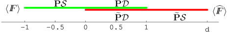
FIG. 1.: The state spaces for Werner and isotropic states are just intervals. Drawn together in one diagram the intersection gives us the space of PPT-states, which is in this case equivalent to the separable space.

Note that by exchanging the roles of $G$ and ${\widetilde{G}}$, we get exactly the same diagram, up to maybe an affine transformation due to a different choice of coordinates: the two diagrams are simply related by taking partial transposes. When $G$ and ${\widetilde{G}}$ are swapped in this way, the picture of ${\bf P}{\cal D}$ remains correct: since $\Theta_{2}{\cal D}={\cal D}$, it suffices to compute the projection of the separable subset for $G$. By definition, the intersection of ${\bf P}{\cal S}$ and $\Theta_{2}{\widetilde{\bf P}}{\cal S}$ is the convex set of $G$-invariant ppt-states. It always contains ${\bf P}{\cal D}$, but this inclusion may be strict. In the simple case of Figure 1 ${\bf P}{\cal D}={\bf P}{\cal S}\cap\Theta_{2}{\widetilde{\bf P}}{\cal S}$, which is the same as saying that the Peres-Horodecki criterion is valid for states invariant under either $G$ or ${\widetilde{G}}$.

D Further examples of symmetry groups

Example 3: Orthogonal groups: $G=OO$.
The two basic examples can be combined into one by taking the intersection of the two groups: $G=UU\cap U\overline{U}$ this is the same as the subgroup of unitaries $U\otimes U$ such that $\overline{U}=U$, i.e., such that $U$ is a real orthogonal matrix. Clearly, both the $UU$-invariant states and the $U\overline{U}$-invariant states will be $G$-invariant, so we know that $G^{\prime}$ is at leastthe algebra generated by $UU^{\prime}$ and $U\overline{U}^{\prime}$, i.e., it contains ${\leavevmode{\rm 1\mkern-5.4muI}},{I\hskip-3.9ptF}$, and $\widehat{I\hskip-3.9ptF}$. Since ${I\hskip-3.9ptF}\widehat{I\hskip-3.9ptF}=\widehat{I\hskip-3.9ptF}{I\hskip-3.9ptF}=\widehat{I\hskip-3.9ptF}$, the linear span of these three is already an algebra, and is spanned by the minimal projections

$$p_{0} = \frac{1}{3}\widehat{I\hskip-3.9ptF}$$ (12)

$$p_{1} = \frac{1}{2}({\leavevmode{\rm 1\mkern-5.4muI}}-{I\hskip-3.9ptF})$$ (13)

$$p_{2} = \frac{1}{2}({\leavevmode{\rm 1\mkern-5.4muI}}-{I\hskip-3.9ptF})-\frac{1}{3}\widehat{I\hskip-3.9ptF}\;,$$ (14)

which corresponds precisely to the decomposition of a general $3\times 3$-matrix into multiple of the identity, antisymmetric part, and symmetric traceless part. This decomposition of tensor operators with respect to the orthogonal group is well known, so we have identified $G^{\prime}$.

The extremal $G$-invariant states corresponding to these three minimal projections are plotted in Figure 2 in a coordinate system whose axes represent the expectations of ${I\hskip-3.9ptF}$ and $\widehat{I\hskip-3.9ptF}$, respectively. The plane of this drawing should be considered as the hermitian $G$-invariant operators of trace one. This plane is mapped into itself by partial transposition (since $G={\widetilde{G}}$), and the coordinates are chosen such that partial transposition is simply the reflection along the main diagonal.

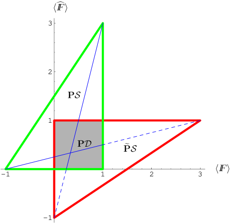
FIG. 2.: State spaces for $OO$ and $O\bar{O}$ invariant states plotted for $d=3$. The $UU$ and $U\overline{U}$ invariant states are drawn as thin lines.

The intersection of ${\bf P}{\cal S}$ and ${\widetilde{\bf P}}{\cal S}$ is the square $[0,1]\times[0,1]$. Is the Peres-Horodecki criterion valid for these states? All we have to do to check this is to try to get some pure product states, whose expectations of ${I\hskip-3.9ptF}$ and $\widehat{I\hskip-3.9ptF}$ fall on the corners of this square. For a product vector $\phi\otimes\psi$ we get the pair of expectations

$$\Bigl{(}|\langle\phi|\psi\rangle|^{2}\;,\ |\langle\phi|\overline{\psi}\rangle|^{2}\Bigr{)}\;.$$

Here $\overline{\psi}$ denotes the complex conjugate of $\psi$ in a basis in which the representation is real. Now the point $(1,1)$ in the square is obtained, whenever $\phi=\psi$ is real, the point $(0,0)$ is obtained when $\phi$ and $\psi$ are real and orthogonal, and the point $(1,0)$ is obtained when $\psi=\phi$, and $\langle\phi|\overline{\phi}\rangle=0$, for example $\phi=(1,i,0)/\sqrt{2}$. Symmetrically we get $(0,1)$ with the same $\phi$ and $\psi=\overline{\phi}$. Hence all four corners are in ${\bf P}{\cal D}$, and as this is a convex set we must have ${\bf P}{\cal D}={\bf P}{\cal S}\cap\Theta_{2}({\widetilde{\bf P}}{\cal S})$.

Example 4: $SU_{2}$-representations.
A class of examples, in which arbitrary dimensions of ${\cal H}_{1}$ and ${\cal H}_{2}$ can occur is the following. Let $u\mapsto{\cal D}^{j}_{u}$ denote the spin $j$ irreducible representation of $SU_{2}$. Then we can take

$$G=\big{\{}{\cal D}^{j_{1}}_{u}\otimes{\cal D}^{j_{2}}_{u}\big{|}u\in SU_{2}\big{\}}\;,$$ (15)

where $(2j_{k}+1)$ is the dimension of ${\cal H}_{k}$ ($k=1,2$). Since the $j_{k}$ also take half-integer values, these dimensions can be any natural number $\geq 1$. It is known from just about any quantum mechanics course (under the key word “addition of angular momenta”) that the tensor product representation ${\cal D}^{j_{1}}\otimes{\cal D}^{j_{2}}$ is decomposed into the direct sum of the irreducible representations ${\cal D}^{s}$ with $s=|j_{1}-j_{2}|,|j_{1}-j_{2}|+1,\ldots(j_{1}+j_{2})$, each of these representations appearing with multiplicity $1$. Therefore, the commutant of $G$ is spanned by the projections onto these subspaces, and is an abelian algebra.

Note that since the spin-$1$ representation of $SU_{2}$ is the orthogonal group in $3$ dimensions, the case $j_{1}=j_{2}=1$ corresponds precisely to the previous example with $d=3$. We have no general expression for the separable subsets, nor even for the partially transposed sets in these examples. We believe, however, that this class of examples deserves further investigation.

Example 5: Bell diagonal states.
In this example we show that the group $G$ can also be abelian, and we make contact with a well investigated structure of the two qubit system. So let ${\cal H}_{1}={\cal H}_{2}={\leavevmode\hbox{\kern 3.00003pt\vrule height=6.45831pt,depth=-0.43057pt,width=0.2pt\kern-3.00003pt\rm C}}^{2}$, and let $\sigma_{k}$, $k=1,2,3$ be the Pauli matrices, and $\sigma_{0}={\leavevmode{\rm 1\mkern-5.4muI}}$. Then the set

$$G=\{{\leavevmode{\rm 1\mkern-5.4muI}},\;-\sigma_{1}\otimes\sigma_{1},\;-\sigma_{2}\otimes\sigma_{2},\;-\sigma_{3}\otimes\sigma_{3}\}$$ (16)

forms a group, which is isomorphic to the Klein $4$-group, and abelian ($G\subset G^{\prime}$). It is even maximally abelian, i.e, the algebra $G^{\prime\prime}$ generated by $G$ is equal to, and not just contained in $G^{\prime}$. The minimal projections in $G^{\prime}$ are $|\Psi_{k}\rangle\!\langle\Psi_{k}|$, $k=0,1,2,3$, where the $\Psi_{k}$ are the magical Bell Basis [9, 16]: $\Psi_{0}=(|11\rangle+|22\rangle)/\sqrt{2}$, and $\Psi_{k}=i({\leavevmode{\rm 1\mkern-5.4muI}}\otimes\sigma_{k})\Psi_{0}$ for $k=1,2,3$. In this basis the group elements and their negatives are the diagonal operators with diagonal elements $\pm 1$, of which an even number are $-1$. Hence the $G$-invariant states are the tetrahedron of density operators which are diagonal in Bell Basis.

The partial transpose is easy to compute: only $\sigma_{2}$ changes sign under transposition. Hence if we draw the state space in a coordinate system, whose three axes are the expectations of the group elements $-\sigma_{k}\otimes\sigma_{k}$ ($k=1,2,3$), the Bell states are the corners $(1,1,1)$, $(1,-1,-1)$, $(-1,-1,1)$, and $(-1,1,-1)$ of the unit cube, from which their partial transposes are obtained by mirror reflection $x_{2}\mapsto-x_{2}$. That is, the partially transposed states occupy the remaining four corners of the unit cube. The ppt-subset, which is equal to the separable subset since we are in $2\otimes 2$ dimensions, is hence the intersection of two tetrahedra, and is easily seen to be an octahedron.

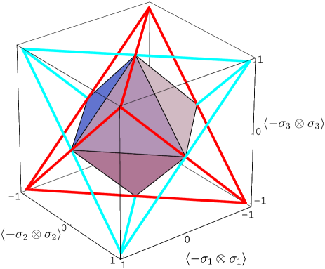
FIG. 3.: State spaces for Bell diagonal states.

Example 6: Finite Weyl Systems.
In the examples so far the groups $G$ and ${\widetilde{G}}$ were isomorphic or even equal. In this example, which extends the previous one, we see that the two groups and their commutants can be very different.

We let $d$ be an integer, and introduce on ${\leavevmode\hbox{\kern 3.00003pt\vrule height=6.45831pt,depth=-0.43057pt,width=0.2pt\kern-3.00003pt\rm C}}^{d}$ the Weyl operators, given by

$$W(x,y)|z\rangle=\omega^{xz}|z-y\rangle\;,$$ (17)

where $\omega=\exp(2\pi i/p)$. These are unitary, and satisfy the “Weyl relations”

$$W(x_{1},y_{1})W(x_{2},y_{2})=\omega^{-x_{1}y_{2}}W(x_{1}+x_{2},y_{1}+y_{2})\;.$$ (18)

Hence these operators, together with the $p^{\rm th}$ roots of unity form a group. On ${\leavevmode\hbox{\kern 3.00003pt\vrule height=6.45831pt,depth=-0.43057pt,width=0.2pt\kern-3.00003pt\rm C}}^{d}\otimes{\leavevmode\hbox{\kern 3.00003pt\vrule height=6.45831pt,depth=-0.43057pt,width=0.2pt\kern-3.00003pt\rm C}}^{d}$ we introduce the operators $W(x_{1},y_{1},x_{2},y_{2})\equiv W(x_{1},y_{1})\otimes W(x_{2},y_{2})$, and take

$$G=\big{\{}\omega^{z}W(x,y,x,y)\;\big{|}x,y,z=0,\ldots,d-1\big{\}}\;.$$ (19)

The commutant is readily computed from the Weyl relations to be

$$G^{\prime}={\rm span}\big{\{}W(x,y,-x,-y)\;\big{|}x,y=0,\ldots,d-1\big{\}}\;.$$ (20)

The Weyl operators in $G^{\prime}$ satisfy Weyl relations with $\omega$ replaced by $\omega^{2}$. If $d$ is odd, such relations are equivalent to the Weyl relations (18) for a $d$-dimensional system, and hence $G^{\prime}$ is isomorphic to the $d\times d$-matrices.

On the other hand, complex conjugation of $W(x,y)$ just inverts the sign of $x$, so ${\widetilde{G}}$ contains the Weyl operators $W(x,y,-x,y)$. But this time, rather than getting twice the Weyl phase, the phases cancel, and ${\widetilde{G}}$ is abelian. One also verifies that

$${\widetilde{G}}^{\prime}={\rm span}\big{\{}W(x,y,-x,y)\;\big{|}x,y=0,\ldots,d-1\big{\}}\;.$$ (21)

is spanned by ${\widetilde{G}}$, so this algebra is even maximally abelian: it contains $d^{2}$ one-dimensional projections, which thus form the extreme points of ${\widetilde{\bf P}}{\cal S}$. Hence we get the following picture: the set ${\bf P}{\cal S}$ of $G$-invariant states is isomorphic to the space of $d\times d$-density operators, and the $G$-invariant operators with positive partial transpose are a simplex spanned by $9$ extreme points, which are mapped into each other by the action of a $d\times d$ Weyl system. The intersection ${\bf P}{\cal S}\cap\Theta_{2}({\widetilde{\bf P}}{\cal S})$ is a rather complicated object. We do not know yet whether it differs from ${\bf P}{\cal D}$.

Example 7: Tensor products.
Additivity problems for entanglement (see Section III C for a brief survey) concern tensor products of bipartite states, which are taken in such a way as to preserve the splitting between Alice and Bob. Thus in the simplest case we have four subsystems, described in Hilbert spaces ${\cal H}_{i},{\cal K}_{i}$, $i=1,2$, such that systems ${\cal H}_{1}$ and ${\cal K}_{1}$ belong to Alice, systems ${\cal H}_{2}$ and ${\cal K}_{2}$ belong to Bob, and such that the systems in ${\cal H}_{i}$ are prepared together according to a density matrix $\rho$ on ${\cal H}_{1}\otimes{\cal H}_{2}$ and, similarly, the remaining systems are prepared according to $\sigma$, a density operator on ${\cal K}_{1}\otimes{\cal K}_{2}$. We wish to study the entanglement properties of $\rho\otimes\sigma$, when both these density matrices are assumed to be invariant under suitable groups of local unitaries.

Let us denote by $G$ (resp. $H$) the group of local unitaries on ${\cal H}_{1}\otimes{\cal H}_{2}$ (resp. by ${\cal K}_{1}\otimes{\cal K}_{2}$), and assume $\rho$ and $\sigma$ to be invariant under the respective group. Then, clearly, $\rho\otimes\sigma$ is invariant under all unitaries $U_{1}\otimes U_{2}\otimes V_{1}\otimes V_{2}$, where $U_{1}\otimes U_{2}\in G$ and $V_{1}\otimes V_{2}\in H$. These again form a group of local unitaries, denoted by $G\otimes H$, where “local” is understood in the sense of the Alice$-$Bob splitting of the system, i.e., the unitary $U_{1}\otimes V_{1}$ acts on Alice’s side and $U_{2}\otimes V_{2}$ on Bob’s. In this sense the product state is invariant under the group $G\otimes H$ of local unitaries, and we can apply the methods developed below to compute various entanglement measures for it.

Computing the commutant $(G\otimes H)^{\prime}$ is easy, because we do not have to look at the Alice$-$Bob splitting of the Hilbert space. In fact, we can invoke the “Commutation Theorem” for von Neumann algebras to get

$$(G\otimes H)^{\prime}=G^{\prime}\otimes H^{\prime}\;,$$ (22)

where the notation on the right hand side is the tensor product of algebras, i.e., this is the set of all linear combinations of elements of the form $A\otimes B$ where $A\in G^{\prime}$ acts on the first two and $B\in H^{\prime}$ acts on the second two factors of ${\cal H}_{1}\otimes{\cal H}_{2}\otimes{\cal K}_{1}\otimes{\cal K}_{2}$. In particular, if $G^{\prime}$ and $H^{\prime}$ are abelian, so is $G^{\prime}\otimes H^{\prime}$, and we can readily compute the minimal projections, which correspond to the extremal invariant states: if $p_{\alpha}$ are the minimal projections of $G^{\prime}$ and $q_{\beta}$ are those of $H^{\prime}$, then the minimal projections of $G^{\prime}\otimes H^{\prime}$ are all $p_{\alpha}\otimes q_{\beta}$.

Partial transposition also behaves naturally with respect to tensor products, which implies that $(G\otimes H){\widetilde{\ }}={\widetilde{G}}\otimes{\widetilde{H}}$, and allows us to compute in a simple way the $(G\otimes H)$-invariant states with positive partial transpose from the corresponding data of $G$ and $H$. However, for the determination of ${\bf P}{\cal D}$ no such shortcut exists.

We illustrate this in the example, which we will also use for the counterexample to additivity of the relative entropy of entanglement announced in the Introduction. For this we take $G=H=UU$, with a one-particle space ${\cal H}_{1}={\cal H}_{2}={\cal K}_{1}={\cal K}_{2}={\leavevmode\hbox{\kern 3.00003pt\vrule height=6.45831pt,depth=-0.43057pt,width=0.2pt\kern-3.00003pt\rm C}}^{d}$, for any dimension $d<\infty$. The extreme points of the state space of $G^{\prime}$ are given by the normalized projections

$$\rho_{\pm}=\frac{1}{d(d\pm 1)}({\leavevmode{\rm 1\mkern-5.4muI}}\pm{I\hskip-3.9ptF})\;.$$ (23)

Hence the state space of the abelian algebra $(G^{\prime}\otimes H^{\prime})$ is spanned by the four states $\rho_{s_{1}}\otimes\rho_{s_{2}}$, $s_{1},s_{2}=\pm$ and is a tetrahedron. A convenient coordinate system is given by the expectations of the three operators

$$F_{1} = {I\hskip-3.9ptF}\otimes{\leavevmode{\rm 1\mkern-5.4muI}}$$ (24)

$$F_{2} = {\leavevmode{\rm 1\mkern-5.4muI}}\otimes{I\hskip-3.9ptF}$$ (25)

$$F_{12} = {I\hskip-3.9ptF}\otimes{I\hskip-3.9ptF}\;.$$ (26)

The four extreme points are then on the edges of the unit cube: $\rho_{s_{1}}\otimes\rho_{s_{2}}$ has expectation triple $(s_{1},s_{2},s_{1}s_{2})$. This is drawn in Figure 4.

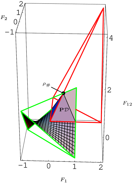
FIG. 4.: State space for $UUVV$-invariant states plotted for dimension $d=3$.

The extreme points are special instances of product states: when $\rho,\sigma$ are $UU$-invariant states with flip expectations $f_{1}$ and $f_{2}$, respectively, the product state $\rho\otimes\sigma$ has coordinates $(f_{1},f_{2},f_{1}f_{2})$. Hence the manifold of product states is embedded in the state space as a piece of hyperboloid. Partial transposition turns the flip operators (24) into their counterparts using $\widehat{I\hskip-3.9ptF}$ instead of ${I\hskip-3.9ptF}$. Hence the operators with positive partial transposes are represented in the diagram by a tetrahedron with vertices $(0,0,0)$, $(0,d,0)$, $(d,0,0)$, and $(d,d,d^{2})$. The intersection, i.e., the set of states with trace equal to one and positive partial transpose (represented in Figure 4 as a solid) is a polytope with the five extreme points $(0,0,0)$, $(0,1,0)$, $(1,0,0)$, $(1,1,1)$, and, on the line connecting the origin to the point $(d,d,d^{2})$, the point $(1/d,1/d,1)$. The density operator corresponding to this last point is

$$\rho_{\#}=\frac{d+1}{2d}\rho_{+}\otimes\rho_{+}+\frac{d-1}{2d}\rho_{-}\otimes\rho_{-}\;.$$ (27)

It turns out that $\rho_{\#}$ is separable: Let $\Phi=d^{-1/2}\sum_{k}|kk\rangle$ be a maximally entangled vector, and consider a pure state with vector $\Psi=\Phi_{\text{Alice}}\otimes\Phi_{\text{Bob}}$. Note that this is a tensor product with respect to the splitting Alice$-$Bob, i.e., $13|24$ rather than the splitting between pair 1 and pair 2, i.e., $12|34$. We claim that upon twirling this pure state becomes $\rho_{\#}$. For this we only need to evaluate the expectations of the three operators (24), and compare with those of $\rho_{\#}$. Clearly, $\Psi$ is a symmetric product (Bose-) vector with respect to the total flip $F_{12}$, hence this operator has expectation $1$. The expectations of $F_{1}$ and $F_{2}$ are equal to

$$\langle\Psi|F_{1}\Psi\rangle = \frac{1}{d^{2}}\sum\langle ijij|({I\hskip-3.9ptF}\otimes{\leavevmode{\rm 1\mkern-5.4muI}})|k\ell k\ell\rangle$$

$$= \frac{1}{d^{2}}\sum_{i,j,k,\ell}\langle ijij|\ell kk\ell\rangle=\frac{1}{d}\;.$$

Since the other four extreme points are separable as tensor products of separable states, we conclude that all ppt-states are separable in this example, so the solid in Figure 4 also represents the separable subset.

Example 8: Tripartite symmetry: $U\otimes(U\otimes U)$.

The idea of symmetry can also be used to study multi-partite entanglement. A natural choice of symmetry group is the group of all unitaries of the form $U\otimes U\otimes U$. The resulting five dimensional state space has been studied in great detail in [4]. This study also has a bipartite chapter, where this group is considered as a group of local unitaries $U\otimes(U\otimes U)$ in the sense of the present paper. The set of separable states is strictly smaller than the set of states with positive partial transposes. However, if we enlarge the group to include the unitary ${\leavevmode{\rm 1\mkern-5.4muI}}\otimes{I\hskip-3.9ptF}$, the two once again coincide, forming a tetrahedron.

III Entanglement measures and additivity

A Entanglement of Formation and the convex hull construction for functions

The entanglement of a pure state is well described by the von Neumann entropy of its restricted density operator. Thus for a pure state $\rho=|\Psi\rangle\!\langle\Psi|$ such that $\Psi$ is expressed in Schmidt form as $\Psi=\sum_{k}\sqrt{c_{k}}e_{k}\otimes e_{k}^{\prime}$, we have

$$E(\rho) = \sum_{k}\eta(c_{k})\quad\text{with}$$ (28)

$$\eta(t) = -t\log(t)\;.$$ (29)

The entanglement of formation is a specific extension of this function to mixed states. The extension method is a general one, known as the convex hull construction for functions, and since we will need this construction for stating our main result, we will briefly review it.

So let $K$ be a compact convex set, let $M\subset K$ be an arbitrary subset, and let $f:M\to{{\rm I\mkern-3.6muR}}\cup\{+\infty\}$. We then define a function ${\rm co}f:K\to{{\rm I\mkern-3.6muR}}\cup\{+\infty\}$ by

$${\rm co}f(x)=\inf\Big{\{}\sum_{i}\lambda_{i}f(s_{i})\Big{|}s_{i}\in M,\ \sum_{i}\lambda_{i}s_{i}=x\Big{\}}\;,$$ (30)

where the infimum is over all convex combinations with $\lambda_{i}\geq 0$, $\sum_{i}\lambda_{i}=1$, and by convention the infimum over an empty set is $+\infty$. The name “convex hull” of this function is due to the property that ${\rm co}f$ is the largest convex function, which is $\leq f$ at all points, where $f$ is defined. Another way of putting this is to say that the “supergraph” of ${\rm co}f$, i.e., $\big{\{}(x,r)\in K\times{{\rm I\mkern-3.6muR}}\big{|}r\geq{\rm co}f(x)\big{\}}$, is the convex hull (as a subset of $K\times{{\rm I\mkern-3.6muR}}$) of $\big{\{}(x,r)\in K\times{{\rm I\mkern-3.6muR}}\big{|}x\in M,\ r\geq f(x)\big{\}}$.

In this notation, the usual definition [9] of entanglement of formation is then

$$E_{\rm F}(\rho)=({\rm co}E)(\rho)\;,$$ (31)

where on the right hand side $E$ is understood as the function (28) defined only on the submanifold $M\subset{\cal S}({\cal H}_{1}\otimes{\cal H}_{2})$ of pure states.

B Relative Entropy of Entanglement

Another measure of entanglement, originally proposed in [7] is based on the idea that entanglement should be zero for separable density operators (see Equation (5)), and should increase as we move away from ${\cal D}$. Such a function might be viewed as measuring some kind of distance of the state to the set ${\cal D}$ of separable states. If one takes this idea literally, and uses the relative entropy [19]

$$\SS(\rho,\sigma)={\rm tr}\rho(\log\rho-\log\sigma)$$ (32)

to measure the “distance”, one arrives at the relative entropy of entanglement

$$E_{\rm RE}(\rho)=\inf\big{\{}\SS(\rho,\sigma)\big{|}\sigma\in{\cal D}\big{\}}\;.$$ (33)

Initially, other distance functions have also been used to define measures of entanglement. However, the one based on the relative entropy is the only proposal, which coincides on pure states with the “canonical” choice described in Equation (28). Since $E_{\rm RE}$ is easily shown to be convex, it must be smaller than the largest convex function with this property, namely $E_{\rm F}$. Another reason to prefer relative entropy over other distance-like functionals is that it has good additivity properties. The hope that $E_{\rm RE}$ might be additive was borne out by initial explorations, and has become a folk conjecture in the field. However, we will give a counterexample below.

C Additivity

A key problem in the current discussion of entanglement measures is the question, which of these are “additive” in the following sense: if $\rho,\sigma$ are bipartite states on the Hilbert spaces ${\cal H}_{1}\otimes{\cal H}_{2}$ and ${\cal K}_{1}\otimes{\cal K}_{2}$, then $\rho\otimes\sigma$ is a state on ${\cal H}_{1}\otimes{\cal H}_{2}\otimes{\cal K}_{1}\otimes{\cal K}_{2}$. After sorting the factors in this tensor product into spaces ${\cal H}_{1},{\cal K}_{1}$ belonging to Alice and ${\cal H}_{2},{\cal K}_{2}$ belonging to Bob, we can consider $\rho\otimes\sigma$ as a bipartite state on $({\cal H}_{1}\otimes{\cal K}_{1})\otimes({\cal H}_{2}\otimes{\cal K}_{2})$. This corresponds precisely to the situation of a source distributing particles to Alice and Bob, $\rho\otimes\sigma$, and similar larger tensor products, being interpreted as the state obtained by letting Alice and Bob collect their respective particles. Additivity of an entanglement measure $E$ is then the equation

$$E(\rho\otimes\sigma)=E(\rho)+E(\sigma)\;.$$ (34)

We speak of subadditivity if “$\leq$” holds instead of equality here. Both $E_{\rm RE}$ and $E_{\rm F}$ are defined as infima, and for a product we can insert tensor products of convex decompositions or closest separable points into these infima, and use the additivity properties of entropy to get subadditivity in both cases. It is the converse inequality, which presents all the difficulties, i.e., the statement that in these minimization problems the tensor product solutions (and not some entangled options) are already the best.

Additivity of an entanglement functional is a strong expression of the resource character of entanglement. According to an additive functional, sharing two particles from the same preparing device is exactly “twice as useful” to Alice and Bob as having just one. Here preparing two pairs means preparing independent pairs, expressed by the tensor product in (34). It is interesting to investigate the influence of correlations and entanglement between the different pairs. On the one hand, Alice and Bob might not be aware of such correlations, and use the pairs as if they were independent. On the other hand, they might make use of the exact form of the state, including all correlations. Is the second possibility always preferable? Entanglement functionals answering this question with “yes” have a property stronger than additivity, called strong superadditivity. It is written as

$$E(\rho)\geq E(\rho_{\cal H})+E(\rho_{\cal K})\;,$$ (35)

where $\rho$ is a density operator for two pairs (four particles altogether), and $\rho_{\cal H}$ and $\rho_{\cal K}$ are the restrictions to the first and second pair. An entanglement functional satisfying this as well as subadditivity is clearly additive. Since additivity is already difficult to decide, it is clear that strong superadditivity is not known for any of the standard measures of entanglement.

One case of strong superadditivity is satisfied both for $E_{\rm F}$ and $E_{\rm RE}$, and we establish this property here in order to get a more focused search for counterexamples later on: We claim that (35) holds, whenever $\rho_{\cal K}$ is separable, in which case, of course, the second term on the right vanishes (as a special case of additivity, when $\rho_{\cal K}$ is even a product, this was noted recently in [18]). We will show this by establishing another property, called monotonicity: for both $E=E_{\rm F}$ and $E=E_{\rm RE}$, we claim

$$E(\rho)\geq E(\rho_{\cal H})\;.$$ (36)

Monotonicity for $E_{\rm RE}$ follows readily from a similar property of the relative entropy: if $\rho_{\cal H},\sigma_{\cal H}$ denote the restrictions of states $\rho,\sigma$ to the same subsystem, then $\SS(\rho_{\cal H},\sigma_{\cal H})\leq\SS(\rho,\sigma)$. But if $\sigma$ is separable in (33), then so is its restriction $\sigma_{\cal H}$. The infimum over all separable states on ${\cal H}_{1}\otimes{\cal H}_{2}$ is still smaller, hence monotonicity holds.

Monotonicity for $E_{\rm F}$ is similar: We may do the reduction in stages, i.e., first reduce Alice’s and then Bob’s system, and because $E_{\rm F}$ symmetric with respect to the exchange of Alice and Bob, it suffices to consider the case of a reduction on only one side, i.e., the restriction from ${\cal H}_{1}\otimes({\cal H}_{2}\otimes{\cal K}_{2})$ to ${\cal H}_{1}\otimes{\cal H}_{2}$.

Let $\rho$ be a state on ${\cal H}_{1}\otimes({\cal H}_{2}\otimes{\cal K}_{2})$ and $\rho^{\prime}$ its restriction to ${\cal H}_{1}\otimes{\cal H}_{2}$.

Consider the states $s_{i}$ on the larger space appearing in the minimizing convex decomposition of $\rho$, and let $s_{i}^{\prime}$ denote their restrictions to ${\cal H}_{1}\otimes{\cal H}_{2}$. Of course, both $s_{i}$ and $s_{i}^{\prime}$ have the same restriction to the first factor ${\cal H}_{1}$. Hence

$$E_{\rm F}(\rho)=\sum_{i}\lambda_{i}f(s_{i}^{\prime})\;,$$ (37)

where $f(\sigma)$ denotes the von Neumann entropy of the restriction of a state $\sigma$ to ${\cal H}_{1}$, and $\sum_{i}\lambda_{i}s_{i}^{\prime}=\rho^{\prime}$. Because the entropy of the restriction is a concave function, the value of the sum (37) can be made smaller by replacing each $s_{i}^{\prime}$ with a decomposition into pure states on ${\cal H}_{1}\otimes{\cal H}_{2}$. Minimizing over all such decompositions of $\rho^{\prime}$ yields $E_{\rm F}(\rho^{\prime})$, which is hence smaller than $E_{\rm F}(\rho)$.

IV Entanglement of formation

A Simplified computation

Our method for computing the entanglement of formation can also be explained in the general setting of the convex hull construction in Subsection III A, and this is perhaps the best way to see the geometrical content. So in an addition to a subset $M\subset K$ of a compact convex set and a function $f:M\to{{\rm I\mkern-3.6muR}}\cup\{+\infty\}$, consider a compact group $G$ of symmetries acting on $K$ by transformations $\alpha_{U}:K\to K$, which preserve convex combinations. We also assume that $\alpha_{U}M\subset M$, and $f(\alpha_{U}s)=f(s)$ for $s\in M$. All this is readily verified for $\alpha_{U}(A)=UAU^{*}$ and $f$ the entanglement defined on the subset $M\subset K$ of pure bipartite states. Our task is to compute ${\rm co}f(x)$ for all $G$-invariant $x\in K$, i.e., those with $\alpha_{U}(x)=x$ for all $U\in G$.

Since the integral with respect to the Haar measure is itself a convex combination, we can define, as before, the projection ${\bf P}:K\to K$ by ${\bf P}x=\int\!dU\ \alpha_{U}(x)$. The set of projected points ${\bf P}x$ will be denoted by ${\bf P}K$. Usually, this will be a much lower dimensional object than $K$, so we will try to reduce the computation of the infimum (30), which involves a variation over all convex decompositions of $x$ in the high dimensional set $K$ to a computation, which can be done entirely in ${\bf P}K$. To this end, we define the function $\varepsilon:{\bf P}K\to{{\rm I\mkern-3.6muR}}\cup\{+\infty\}$ by

$$\varepsilon(x)=\inf\big{\{}f(s)\big{|}s\in M,\ {\bf P}s=x\big{\}}\;,$$ (38)

again with the convention that the infimum over the empty set is $+\infty$. Then the main result of this subsection is that, for $x\in{\bf P}K$,

$${\rm co}f(x)={\rm co}\;\varepsilon(x)\;,$$ (39)

where the convex hull on the left is defined by (30), but the convex hull on the right is now to be computed in the convex subset ${\bf P}K$.

We thus arrive at the following recipe for computing the entanglement of formation of $G$-invariant states:

• Find, for every state $\rho\in{\bf P}{\cal S}$, the set $M_{\rho}$ of pure states $\sigma$ such that ${\bf P}\sigma=\rho$.

• Compute

  $$\varepsilon(\rho):=\inf\big{\{}E(\sigma)\big{|}\sigma\in M_{\rho}\big{\}}\;.$$ (40)

• For later use try to get a good understanding of the pure states achieving this minimum.

• Compute the convex hull of the function (40).

The following simplifications are sometimes possible: first of all, all pure states in an orbit of $G$ give the same value of $E$, hence we may replace $M_{\rho}$ by a suitably parametrized subset containing at least one element from every orbit. At this stage it is sometimes already possible to discard further states, in favour of others “obviously” giving a smaller value of $E$. The final stage is sometimes carried out by showing that the function $\varepsilon$ is convex to begin with, but, as we will see, this is not always the case.

The remainder of this subsection is devoted to the proof of Equation (39). We will proceed by showing that both sides are equal to

$$Z=\inf\Big{\{}\sum_{i}\lambda_{i}f(s_{i})\Big{|}s_{i}\in M,\ \sum_{i}\lambda_{i}{\bf P}s_{i}=x\Big{\}}\;.$$ (41)

Indeed, the only difference between (41) and (30) is that in (41) a weaker condition is demanded on the $s_{i}$. Hence more $s_{i}$ are admissible, and this infimum is smaller, $Z\leq{\rm co}f(x)$. On the other hand, if $s_{i}$ satisfying the constraint for $Z$ are given, inserting the definition of ${\bf P}$ produces a convex combination giving $x$, namely the combination of the states $\alpha_{U}(s_{i})$, labeled by the pair $(i,U)$, and weighted with $\sum_{i}\lambda_{i}\int\!dU\$. This convex combination is admissible for the infimum defining ${\rm co}f$, and gives the value $\sum_{i}\lambda_{i}\int\!dU\ f(\alpha_{U}(s_{i}))=\sum_{i}\lambda_{i}\int\!dU\ f(s_{i})=\sum_{i}\lambda_{i}f(s_{i})$, where we have used the invariance property of $f$ and the normalization of the Haar measure. Hence all numbers arising in the infimum (41) also appear in the infimum (30), which proves that $Z\leq{\rm co}f(x)$, hence $Z={\rm co}f(x)$. In order to prove the equality $Z={\rm co}\;\varepsilon(x)$ just note that in the infimum (41) the constraint is only in terms of ${\bf P}s_{i}$, whereas the functional to be minimized involves $f(s_{i})$. Therefore we can compute the infimum (41) in stages, by first fixing all ${\bf P}s_{i}$ and minimizing each $f(s_{i})$ under this constraint, which amounts to replacing $f$ by $\varepsilon$, and then varying over the ${\bf P}s_{i}$, which is the infimum defining ${\rm co}\;\varepsilon$. Hence ${\rm co}\;\varepsilon(x)=Z={\rm co}f(x)$.

B Extending the computation to some non-symmetric states

It is a basic feature of the convex hull that whenever the infimum in (30) is found at a non-trivial convex combination, there is a “flat piece” in the graph of ${\rm co}f$, i.e., ${\rm co}f$ is also known on the convex hull of the minimizing $s_{i}$ [11]. The geometrical meaning of this elementary observation is immediately clear from low dimensional pictures. It is also easy to prove in general:

Suppose that $\sum_{i}\lambda_{i}s_{i}=x$ is a convex decomposition of $x$ (with $\lambda_{i}>0$) minimizing $\sum_{i}\lambda_{i}f(s_{i})$, and let $x^{\prime}=\sum_{i}\lambda^{\prime}_{i}s_{i}$ be another convex combination of the same points $s_{i}$. We claim that this convex combination solves the minimization problem for ${\rm co}f(x^{\prime})$, i.e.,

$${\rm co}f(x^{\prime})=\sum_{i}\lambda^{\prime}_{i}f(s_{i})\;.$$ (42)

Indeed, let $x^{\prime}=\sum_{j}\mu_{j}t_{j}$ be any convex combination with $t_{j}\in M$. Then we can find a small number $\varepsilon>0$ such that $(\lambda_{i}-\varepsilon\lambda^{\prime}_{i})\geq 0$ for all $i$. Hence

$$x=\sum_{i}(\lambda_{i}-\varepsilon\lambda^{\prime}_{i})s_{i}+\sum_{j}\varepsilon\mu_{j}t_{j}$$

is a convex combination of elements from $M$ representing $x$. But since the decomposition using only the $s_{i}$ is optimal, we have

$$\sum_{i}(\lambda_{i}-\varepsilon\lambda^{\prime}_{i})f(s_{i})+\sum_{j}\varepsilon\mu_{j}f(t_{j})\geq\sum_{i}\lambda_{i}f(s_{i})\;$$

From this we immediately get the claimed optimality of $x^{\prime}=\sum_{j}\lambda^{\prime}_{j}s_{j}$.

These remarks are especially useful for the case of entanglement of formation, for any mixed state the optimizing convex decomposition necessarily involves several terms. Hence any computation of an entanglement of formation immediately extends to a larger class of states. Therefore, it is of great interest not only to get the value of the entanglement of formation for a given mixed state, but also to find the set of pure states solving the variational problem defining $E_{\rm F}$

The symmetric situation studied in this paper is extreme in this regard: The minimizing sets are always complete orbits of the symmetry group. Therefore we get a fairly large set of non-symmetric mixed states for which the computations below also give the exact value of $E_{\rm F}$.

C Results for $G=UU$

In this subsection we will apply the general method to computing the entanglement of formation for the states of Example 1.

In the first step we have to determine the set $M_{f}$ of vectors $\Phi\in{\cal H}\otimes{\cal H}$ such that $\langle\Phi|{I\hskip-3.9ptF}\Phi\rangle=f$. In terms of the vector components $\Phi_{ij}$ we get

$$\langle\psi|{I\hskip-3.9ptF}\psi\rangle=\sum_{ij}\Phi_{ij}\overline{\Phi}_{ji}\;.$$ (43)

On the other hand, the reduced density operator has components $\rho_{ij}=\sum_{k}\Phi_{ik}\overline{\Phi}_{jk}$ or, in matrix notation, $\rho=\Phi\Phi^{*}$. Here we may introduce a simplification due to $U\otimes U$ symmetry, by choosing $\rho$ diagonal. Note, however, that we can not choose the restriction to the second system, i.e., $\Phi^{T}\bar{\Phi}$ to be diagonal at the same time without loss of generality. In any case, the eigenvalues of $\rho$ become $\rho_{ii}=\sum_{k}|\Phi_{ik}|^{2}$. Hence the pure state entanglement of $\Phi$, which by (28) is the entropy of $\rho$ is

$$E(|\Phi\rangle\!\langle\Phi|)=\sum_{i}\eta\Bigl{(}\sum_{k}|\Phi_{ik}|^{2}\Bigr{)}\;,$$ (44)

where $\eta$ is the entropy function from (29).

For analyzing the variational problem it is useful to consider the contributions of each pair of variables $\Phi_{ij}$ and $\Phi_{ji}$, and of each diagonal element $\Phi_{ii}$ separately. The weights of these contributions are

$$\lambda_{ij} = |\Phi_{ij}|^{2}+|\Phi_{ji}|^{2}\;,\quad\text{for}\ i<j$$ (45)

$$\lambda_{ii} = |\Phi_{ij}|^{2}\;.$$ (46)

The normalized contribution of one such pair or diagonal element to $f$ is

$$f_{ij} = \lambda_{ij}^{-1}\ 2\Re\bigl{(}{\Phi_{ij}}\overline{\Phi_{ji}}\bigr{)}\;,\quad\text{for}\ i<j$$ (47)

$$f_{ii} = 1\;,\quad\text{so that }$$ (48)

$$f = \sum_{i\leq j}\lambda_{ij}f_{ij}\;.$$ (49)

Similarly, we can write the probability distribution $\rho_{11},\ldots,\rho_{dd}$ as a convex combination of probability distributions with respective entropies

$$s_{ij} = H_{2}\Bigl{(}\lambda_{ij}^{-1}|\Phi_{ij}|^{2}\Bigr{)}\;,\quad\text{for}\ i<j$$ (50)

$$s_{ii} = 0\;,$$ (51)

where we have used the abbreviation $H_{2}(p)=\eta(p)+\eta(1-p)$ for the entropy of a two point probability distribution $(p,1-p)$. By concavity of the entropy we have

$$E(|\Phi\rangle\!\langle\Phi|)\geq\sum_{i\leq j}\lambda_{ij}s_{ij}\;.$$ (52)

To find the lower bound on $s_{ij}$ given $f_{ij}$ is just another instance of the variational problem we are solving, albeit with the considerable simplification that only one off-diagonal pair of components of $\Phi$ is non-zero. This leaves the following problem:

Given two complex variables $x,y$ with the constraint $|x|^{2}+|y|^{2}=1$, with $2\Re(x\overline{y})=f$, minimize $s=H_{2}(|x|^{2})$.

Since $s$ is monotonely increasing in $|x|^{2}$ form $0$ to $1/2$, this is equivalent to minimizing $|x|^{2}$, given $f$. The pairs $(|x|^{2},f)$ compatible with the constraints form the convex set

$$\big{\{}(\lambda,f)\big{|}\;|f|\leq 2\sqrt{\lambda(1-\lambda)};\ 0\leq\lambda\leq 1\big{\}}\;.$$

From this we get the minimal admissible $|x|^{2}=(1-\sqrt{1-f^{2}})/2$ in the above two variable variational problem. Hence

$$s_{ij}\geq\varepsilon_{2}(f_{ij})=H_{2}\Bigl{(}\frac{1}{2}\;\bigr{(}1-\sqrt{1-f_{ij}^{2}}\;\bigl{)}\Bigr{)}\;.$$ (53)

This function $\varepsilon_{2}$ can be shown to be convex by explicitly computing the second derivative and expanding logarithms in a power series. Combining the bounds (52), (51), and (53) with the convexity of $\varepsilon_{2}$, we get

$$E(|\Phi\rangle\!\langle\Phi|) \geq \sum_{i<j}\lambda_{ij}\;\varepsilon_{2}(f_{ij})$$

$$\geq \varepsilon_{2}\Bigl{(}\sum_{i<j}\lambda_{ij}\;f_{ij}\Bigr{)}$$

$$= \varepsilon_{2}\bigl{(}f-\sum_{i}\lambda_{ii}\bigr{)}\;.$$

Now suppose that $f\geq 0$. Then we can choose just a single diagonal entry $\Phi_{ii}$ to be non-zero, and find $E(|\Phi\rangle\!\langle\Phi|)=0$, which is clearly the minimum. However, if $f<0$ the last equation shows that letting any diagonal entry $\Phi_{ii}\neq 0$ decreases the argument of $\varepsilon_{2}$ further in a range where this function is monotonely decreasing. Hence the optimum is choosing all $\Phi_{ii}=0$, and allowing only two non-zero components $\Phi_{ij}$ and $\Phi_{ji}$ for some $i\neq j$. This concludes the computation of $E_{\rm F}$ for $UU$-invariant states (see summary below).

However, as noted in Section IV B, knowledge of the minimizers for $\varepsilon$ automatically leads to an extension of the computation to some non-invariant states. Let $x,y$ be a solution of the two variable variational problem with $f={\rm tr}(\rho{I\hskip-3.9ptF})$. Then the minimizing vector is of the form

$$x|12\rangle+y|21\rangle=\bigl{(}x{\leavevmode{\rm 1\mkern-5.4muI}}+y{I\hskip-3.9ptF}\bigr{)}|12\rangle\;.$$ (54)

All $U\otimes U$-translates of this vector will do just as well and appear in the minimizing decomposition of the $UU$-invariant state. Hence all convex combinations of the density operators

$$\bigl{(}x{\leavevmode{\rm 1\mkern-5.4muI}}+y{I\hskip-3.9ptF}\bigr{)}(U\otimes U)|12\rangle\langle 12|(U\otimes U)^{*}\bigl{(}x{\leavevmode{\rm 1\mkern-5.4muI}}+y{I\hskip-3.9ptF}\bigr{)}^{*}$$

with fixed $x,y$, and arbitrary $U$, have the same $E_{\rm F}$. For determining these convex combinations we can drop the outer factors, and afterwards shift the operators found with $(x{\leavevmode{\rm 1\mkern-5.4muI}}+y{I\hskip-3.9ptF}\bigr{)}\in G^{\prime}$. Let

$${\cal F}={\rm co}\big{\{}(U\otimes U)|12\rangle\langle 12|(U\otimes U)^{*}\big{|}U\ \text{unitary}\big{\}}\;.$$ (55)

Clearly, every operator in ${\cal F}$ is a separable density operator with flip expectation zero. Conversely, any operator $\widetilde{\rho}$ with these properties may be decomposed into pure product states $|\phi\otimes\psi\rangle\!\langle\phi\otimes\psi|$. These must also have flip expectation zero, which means that $\phi\perp\psi$, so that there is a unitary $U$ with $\phi\otimes\psi=(U\otimes U)|12\rangle$. Consequently $\widetilde{\rho}\in{\cal F}$.

Hence in order to determine whether for a given $\rho$ we can compute $E_{\rm F}(\rho)$, we transform it to $\widetilde{\rho}$ by the appropriate $(x{\leavevmode{\rm 1\mkern-5.4muI}}+y{I\hskip-3.9ptF})^{-1}$, and then test the separability of $\widetilde{\rho}$.

FIG. 5.: $\varepsilon$-function for $UU$ invariant states.

Let us summarize:

• For the $U\otimes U$-invariant state $\rho$ with
  ${\rm tr}(\rho{I\hskip-3.9ptF})=f\leq 0$, we have

  $$E_{\rm F}(\rho)=H_{2}\Bigl{(}\frac{1}{2}\;\Bigr{(}1-\sqrt{1-f^{2}}\;\Bigl{)}\Bigr{)}\;,$$ (56)

  independently of the dimension $d$ of the underlying Hilbert space. When $f\geq 0$, the state $\rho$ is separable, and $E_{\rm F}(\rho)=0$.

• Let $\rho$ be a (not necessarily invariant) density operator with ${\rm tr}(\rho{I\hskip-3.9ptF})=f$ and $-1<f<0$. Then with suitably chosen $\alpha,\beta\in{{\rm I\mkern-3.6muR}}$

  $$\widetilde{\rho}=(\alpha{\leavevmode{\rm 1\mkern-5.4muI}}+\beta{I\hskip-3.9ptF})^{*}\rho(\alpha{\leavevmode{\rm 1\mkern-5.4muI}}+\beta{I\hskip-3.9ptF})$$ (57)

  is a density operator with ${\rm tr}(\widetilde{\rho}{I\hskip-3.9ptF})=0$. Suppose that $\widetilde{\rho}$ is separable. Then formula (56) also holds for $\rho$.

D Results for $G=U\bar{U}$

The computation of the entanglement of formation for Example 2 is already known [12]. The minimizing pure states are of the form

$$\bigl{(}x{\leavevmode{\rm 1\mkern-5.4muI}}+y\widehat{I\hskip-3.9ptF}\bigr{)}|11\rangle\;,$$ (58)

with real $x,y$.

The extension to non-invariant states works in principle similar to the $UU$-case, but for $d>2$ it is getting a bit more complicated, because the $\varepsilon$-function is not convex anymore.

FIG. 6.: $\varepsilon$-function for $U\overline{U}$ invariant states for $d=2,3,4$. The functions are not convex near the right endpoint for $d\geq 3$.

• For the $U\otimes\overline{U}$-invariant state $\rho$ with
  ${\rm tr}(\rho\widehat{I\hskip-3.9ptF})=f\geq\frac{1}{d}$, we have

  $$E_{\rm F}(\rho)={\rm co}\Bigl{(}H_{2}(\gamma)+(1-\gamma)\log(d-1)\Bigr{)}\;,$$ (59)

  with $\gamma=\frac{1}{d^{2}}\left(\sqrt{f}+\sqrt{(d-1)(d-f)}\right)^{2}$. For $d>2$ we need also to compute the convex hull. When $f<\frac{1}{d}$, the state $\rho$ is separable, and $E_{\rm F}(\rho)=0$.

• Let $\rho$ be a (not necessarily invariant) density operator with ${\rm tr}(\rho\widehat{I\hskip-3.9ptF})=f$, $1<f<d$ and ${\rm co}(\varepsilon(f))=\varepsilon(f)$. Then with suitably chosen $\alpha,\beta\in{{\rm I\mkern-3.6muR}}$

  $$\widetilde{\rho}=(\alpha{\leavevmode{\rm 1\mkern-5.4muI}}+\beta\widehat{I\hskip-3.9ptF})^{*}\rho(\alpha{\leavevmode{\rm 1\mkern-5.4muI}}+\beta\widehat{I\hskip-3.9ptF})$$ (60)

  is a density operator with ${\rm tr}(\widetilde{\rho}\widehat{I\hskip-3.9ptF})=1$. Suppose that $\widetilde{\rho}$ is separable. Then formula (59) also holds for $\rho$.

• If $f$ satisfies ${\rm co}(\varepsilon(f))<\varepsilon(f)$ , the convex hull has a flat section between $f_{1}<f<f_{2}$ where $f_{1},f_{2}$ are the two end points of the flat piece satisfying ${\rm co}(\varepsilon(f_{1/2}))=\varepsilon(f_{1/2})$. We can always find a convex decomposition of $\rho$ in two states with expectation values $f_{1},f_{2}$. If now the above procedure works for these two states, then we have found an optimal decomposition for $\rho$ and can easily compute the entanglement of formation.

E Results for $OO$-invariant states

Here the extension method of Section IV.B turns out to do much of the work. The state space, plotted in Figure 7, is separated in four regions. The separable square and the three triangles $A,B,C$.

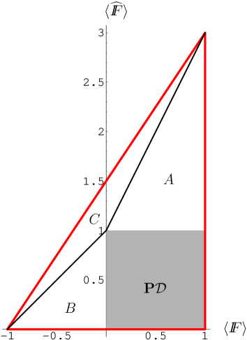
FIG. 7.: The state space for $OO$-invariant states seems to split naturally in four regions. The separable square ${\bf P}{\cal D}$ and the three triangles $A,B,C$.

In order to apply the extension method to the $UU$-invariant states, we have to see which states can be written as $\rho=(x{\leavevmode{\rm 1\mkern-5.4muI}}+y{I\hskip-3.9ptF}){\widetilde{\rho}}(x{\leavevmode{\rm 1\mkern-5.4muI}}+y{I\hskip-3.9ptF})^{*}$, with ${\widetilde{\rho}}$ a separable state with flip expectation zero. If we take for ${\widetilde{\rho}}$ any state at the left edge of the separable square, it is clear that we will get an $OO$-invariant state again. The explicit computation shows that with this method we get $E_{\rm F}(\rho)$ in the full triangle $B$. Note that by this construction $E_{\rm F}(\rho)$ depends only on the expectation $\langle{I\hskip-3.9ptF}\rangle$, and not on $\langle\widehat{I\hskip-3.9ptF}\rangle$ or the dimension $d$. Employing similarly the extension method for $U\overline{U}$ we find $E_{\rm F}(\rho)$ in the triangle $A$, getting a function depending only on $\langle\widehat{I\hskip-3.9ptF}\rangle$ and the dimension, but not on $\langle{I\hskip-3.9ptF}\rangle$.

F Results for Bell-States

The Bell-States were one of the first classes for which entanglement of formation could be calculated [9]. Of course, our method reproduces this result, albeit with a more economical decomposition. This is a feature shared with the Wootters formula[10]. It is a natural question whether the extension method, applied in this basic example, reproduces the Wootters formula. However, it turns out that one gets the result only on state manifolds of lower dimension. We also did not succeed in finding another group of local symmetries, which would give Wootter’s formula in full generality.

V Relative Entropy of Entanglement

A Simplified computation

Symmetry simplifies the computation of the relative entropy of entanglement dramatically: it reduces the variation in (33) from a variation over all separable states $\sigma\in{\cal D}$ to those, which are also $G$-invariant. i.e., when $\rho={\bf P}\rho$, we have

$$E_{\rm RE}(\rho)=\inf\big{\{}\SS(\rho,\sigma)\big{|}\sigma\in{\bf P}{\cal D}\big{\}}\;.$$ (61)

The only ingredients of the proof are the convexity of $\sigma\mapsto\SS(\rho,\sigma)$, the invariance of relative entropy under (local) unitary transformations of both its arguments, and that ${\cal D}$ is a convex set invariant under local unitaries. Indeed, the properties of ${\cal D}$ imply that for any $\sigma$ in the full variational problem, ${\bf P}\sigma\in{\bf P}{\cal D}\subset{\cal D}$ is also a legitimate argument, and the convexity properties of $\SS$ show that this cannot increase $\SS(\rho,\sigma)$. Hence the variation may be restricted as in (61). We have listed the ingredients of the proof so explicitly, because many variations of $E_{\rm RE}$ may be of interest. For example, the “distance” function relative entropy can be replaced by a host of other functions, like norm differences of any kind. The set ${\cal D}$, too, may be replaced, for example by the set of ppt-states, as suggested by Rains [13], who also made similar use of symmetry.

A second simplification concerns the computation of $\SS(\rho,\sigma)$ itself, when both arguments are $G$-invariant. We have seen that $G$-invariant states can be considered as states on the commutant algebra $G^{\prime}$. Now the relative entropy is defined for pairs of states on arbitrary C*-algebras [19], and the form (32) involving density matrices is only the special form valid for a full matrix algebra. Since ${\bf P}$ is a conditional expectation onto $G^{\prime}$, the result does not depend [19] on whether we compute the relative entropy via density matrices, or for the corresponding abstract linear functionals on $G^{\prime}$. Without going into the details for general algebras $G^{\prime}$ here, let us see how this helps in the case when $G^{\prime}$ is abelian, as in most of our examples.

Suppose $p_{\alpha}$, $\alpha=1,\ldots,N$ are the minimal projections of $G^{\prime}$, and denote by $\omega_{\alpha}=({\rm tr}p_{\alpha})^{-1}p_{\alpha}$ the extremal density matrices of ${\bf P}{\cal S}$. Then every $\rho\in{\bf P}{\cal S}$ has a unique representation as a convex combination

$$\rho=\sum_{\alpha}\rho_{\alpha}\omega_{\alpha}=\sum_{\alpha}\frac{\rho_{\alpha}}{{\rm tr}p_{\alpha}}\ p_{\alpha}\;,$$ (62)

where the second expression is at the same time the spectral resolution of $\rho$. If we compute the von Neumann entropy $-{\rm tr}(\rho\log\rho)$ from this, we find a dependence of the result not only on the expectations $\rho_{\alpha}={\rm tr}(\rho p_{\alpha})$, but also on the multiplicities ${\rm tr}(p_{\alpha})$, as is quite familiar from statistical mechanics. On the other hand, the fact that relative entropy can be defined for states on abstract algebras shows that no such dependence can occur for relative entropies. Indeed, the terms involving $\log{\rm tr}(p_{\alpha})$ from $\rho$ and $\sigma$ cancel, and we get

$$\SS(\rho,\sigma)=\sum_{\alpha}\rho_{\alpha}\Bigl{(}\log(\rho_{\alpha})-\log(\sigma_{\alpha})\Bigr{)}\;,$$ (63)

where $\rho_{\alpha}$ and $\sigma_{\alpha}$ are the respective expectations of $p_{\alpha}$.

A typical application is the observation that for $UU$-invariant states the expression for the relative entropy of entanglement can be written down in terms of the ${\rm tr}(\rho F)$, independently of the dimension $d$ of the underlying Hilbert spaces.

For $UU$ and $U\overline{U}$-invariant states the sets of separable states are just intervals, and the definition of relative entropy of entanglement requires a minimization over this interval. However, due to a general property of the relative entropy, the convexity in both arguments, it is clear that the minimum is, in fact always obtained at the endpoint: if $\rho$ is the state whose entanglement we want to calculate, and $\sigma$ is the minimizing separable state, convexity implies

$$\SS(\rho,\lambda\sigma+(1-\lambda)\rho) \leq \lambda\SS(\rho,\sigma)+(1-\lambda)\SS(\rho,\rho)$$

$$= \lambda\SS(\rho,\sigma)\;.$$

Hence if there were any separable state on the straight line segment connecting $\rho$ and $\sigma$, it would give a strictly lower minimum, contradicting the minimality of $\sigma$.

For $UU$ the boundary separable state has ${\rm tr}(\sigma{I\hskip-3.9ptF})=0$, i.e., gives equal weight to the minimal projections. We have to compute the relative entropy with respect to a state with probabilities $(1\pm f)/2$, i.e., the function

$$e_{\rm RE}(f)=\log 2-S\left(\frac{1+f}{2},\frac{1-f}{2}\right)\;,$$ (64)

where we denote by $S(p_{1},\ldots,p_{n})=-\sum_{k}p_{k}\log p_{k}$ the entropy of a probability vector $(p_{1},\ldots,p_{n})$. This function is plotted in Figure 8, and determines the relative entropy of entanglement of $UU$-symmetric states $\rho$ via

$$E_{\rm RE}(\rho)=e_{\rm RE}\bigl{(}{\rm tr}(\rho{I\hskip-3.9ptF})\bigr{)}\;.$$ (65)

FIG. 8.: The relative entropy of entanglement for UU-invariant states.

Similarly, the boundary point $\sigma$ of ${\cal D}$ for $U\overline{U}$ invariant states is given by ${\rm tr}(\sigma\widehat{I\hskip-3.9ptF})=1$. For general $\widehat{f}={\rm tr}(\rho\widehat{I\hskip-3.9ptF})$ the minimal projections have weights $\widehat{f}/d$ and $(1-\widehat{f}/d)$. Hence for $U\overline{U}$-symmetric $\rho$, we have $E_{\rm RE}(\rho)=0$ for $\widehat{f}\leq 1$, and

$$\log d-(1-\frac{\widehat{f}}{d})\log(d-1)-S\Bigl{(}\frac{\widehat{f}}{d},1-\frac{\widehat{f}}{d}\Bigr{)}$$ (66)

otherwise. For comparison with the results of [12], note that $\widehat{f}/d$ is the so called maximally entangled fraction of $\rho$.

Now we look at $OO$-invariant states. The state space and the separable states are drawn in Figure 7. First we look at the state with the coordinates $(1,3)$, which is a maximal entangled state. The separable states, that are minimizing the relative entropy for this state, are the states on the whole line connecting the points $(0,1)$ and $(1,1)$. But now we can find the minimizing separable for any state in the whole triangle $A$. We just have to draw the straight line connecting the coordinates of a given states with the point $(1,3)$. The intersection with the border of ${\bf P}{\cal D}$ is then a minimizer for $(1,3)$ and by the properties of the relative entropy of entanglement also the minimizer for all states on the connecting line. The same argumentation works for the edge point $(-1,0)$ and the separable border between $(0,0)$ and $(0,1)$ giving us all minimizers for the triangle $B$. The whole triangle $C$ has the same minimizer, namely $(0,1)$.

B Counterexample to additivity

To find a counterexample to the additivity of the relative entropy of entanglement we use the group introduced in Example 7 . We also know that additivity will hold for any states where one of the two independently prepared states is separable. So in our example we can restrict to the area, where both expectation values of $F_{1}$ and $F_{2}$ are negative.

For simplicity we increase the group with ${I\hskip-3.9ptF}_{\rm Alice}\otimes{I\hskip-3.9ptF}_{\rm Bob}$ leading us to a smaller commutant only spanned by ${\leavevmode{\rm 1\mkern-5.4muI}}\otimes{\leavevmode{\rm 1\mkern-5.4muI}},{I\hskip-3.9ptF}\otimes{I\hskip-3.9ptF},{\leavevmode{\rm 1\mkern-5.4muI}}\otimes{I\hskip-3.9ptF}+{I\hskip-3.9ptF}\otimes{\leavevmode{\rm 1\mkern-5.4muI}}$. As coordinate system we use the expectation values of

$$F = \frac{1}{2}({\leavevmode{\rm 1\mkern-5.4muI}}\otimes{I\hskip-3.9ptF}+{I\hskip-3.9ptF}\otimes{\leavevmode{\rm 1\mkern-5.4muI}})$$ (67)

$$F_{12} = {I\hskip-3.9ptF}\otimes{I\hskip-3.9ptF}.$$ (68)

The state space is drawn in Figure 9.

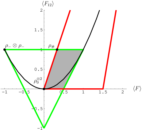
FIG. 9.: State space for $UUVV\&F$-invariant states for $d=3$.

It is just the intersection of the state space of the original group (see Figure 4) with the plane given by $\langle F_{1}\rangle=\langle F_{2}\rangle=\langle F\rangle$. The product states, in the sense of additivity, are given by the line $(\langle F\rangle,\langle F\rangle^{2})$.

The counterexample we want to look at, is the state referring to the coordinates $(-1,1)$, which is given by $\rho_{-}\otimes\rho_{-}$ where $\rho_{-}$ denotes the normalized projection on the antisymmetric subspace of ${\leavevmode\hbox{\kern 3.00003pt\vrule height=6.45831pt,depth=-0.43057pt,width=0.2pt\kern-3.00003pt\rm C}}^{d}\otimes{\leavevmode\hbox{\kern 3.00003pt\vrule height=6.45831pt,depth=-0.43057pt,width=0.2pt\kern-3.00003pt\rm C}}^{d}$. From Equation (65) we know the relative entropy of entanglement for $\rho_{-}$ to be $\log 2$ independent from the dimension $d$. The minimizing state was the state with flip expectation value equal to zero now denoted as $\rho_{0}$. So the expected minimizer for the tensor product would be $\rho_{0}\otimes\rho_{0}$ located on the quadratic product line with the expectation values $(0,0)$. This one gives us the expected value of $\log 4$ for the relative entropy. Now we calculate the relative entropy between $\rho_{-}^{\otimes 2}=\rho_{-}\otimes\rho_{-}$ and $\rho_{\#}$.

$$\SS(\rho_{-}^{\otimes 2},\rho_{\#}) = {\rm tr}(\rho_{-}^{\otimes 2}\log\rho_{-}^{\otimes 2}-\rho_{-}^{\otimes 2}\log\rho_{\#})$$ (69)

$$= {\rm tr}(\rho_{-}^{\otimes 2}\log\rho_{-}^{\otimes 2}-\rho_{-}^{\otimes 2}\log\frac{d-1}{2d}\rho_{-}^{\otimes 2})$$ (70)

$$= -\log\frac{d-1}{2d}=\log 4-\log\frac{2(d-1)}{d}\;.$$ (71)

Indeed the minimum must be attained on the line connecting $\rho_{0}\otimes\rho_{0}$ and $\rho_{\#}$ and it can easily be verified, that the minimum always is attained on $\rho_{\#}$. For $d=2$ the whole line gives the same value and although there exits minimizer not belonging to the product space, additivity holds. For $d>2$ the expectation values of state $\rho_{\#}$ given by $(\frac{1}{d},1)$ shift near to the $F_{12}$ axis and from a geometrical point of view closer to $\rho_{-}\otimes\rho_{-}$. Although the relative entropy is not a real kind of geometrical measure this intuition did not fail. In these cases the additivity is violated with an amount of $\log\frac{2(d-1)}{d}$. For very high dimension $d$ we get the really surprising result $E_{RE}(\rho_{-}\otimes\rho_{-})\simeq E_{RE}(\rho_{-})$.

VI Concluding Remarks

We have concentrated on just two basic entanglement measures. Clearly, there are many more, and for many of them the computation can be simplified for symmetric states. Among these measures of entanglement are the “best separable approximation” of a state [20], the trace norm of the partial transpose [21], the base norm associated with ${\cal D}$ (called cross norm in [22] and absolute robustness in [23]). For distillible entanglement we refer to the recent paper of Rains [6]. Similarly, there is a lot of work left to be done carrying out the programme outlined in this paper for all the groups of local symmetries listed in Section II A.

REFERENCES

- [1] R. F. Werner, Phys. Rev. A 40, 4277 (1989).
- [2] S. Popescu, Phys. Rev. Lett. 72, 797 (1994).
- [3] M. Horodecki and P. Horodecki, Rhys. Rev. A 59, 4206 (1999).
- [4] T. Eggeling and R. F. Werner, quant-ph/0003008.
- [5] W. D r, J.I. Cirac and R. Tarrach, Phys. Rev. Lett. 83, 3562 (1999).
- [6] E. M. Rains, quant-ph/0008047.
- [7] V. Vedral, M.B. Plenio, M.A. Rippin and P. L. Knight, Phys. Rev. Lett. 78, 2275 (1997).
- [8] V. Vedral and M.B. Plenio, Phys. Rev. A 57, 1619(1998).
- [9] C. H. Bennett, D. P. DiVincenzo, J. A. Smolin and W. K. Wootters, Phys. Rev. A 54, 3824 (1996).
- [10] W. K. Wootters, Phys. Rev. Lett. 80, 2245 (1998).
- [11] In the present context this has also been called the roof property of . A. Uhlmann, Open Sys.& Inf. Dyn. 5, 209 (1998).
- [12] B. Terhal and K.G.H. Vollbrecht, Phys. Rev. Lett. 85, 2625 (2000).
- [13] E. M. Rains, Phys. Rev. A 60, 179 (1999).
- [14] H. Weyl, The Classical Groups, (Princeton University, 1946).
- [15] A. Peres, Phys. Rev. Lett. 77, 1413 (1996).
- [16] K.G.H. Vollbrecht and R.F. Werner, J. Math Phys. 41, 6772 (2000).
- [17] M. Takesaki, Theory of Operator Algebras I, (Springer-Verlag 1979).
- [18] F. Benatti and H. Narnhofer, quant-ph/0005126.
- [19] M. Ohya and D. Petz, Quantum Entropy and Its Use, (Springer-Verlag 1993).
- [20] M. Lewenstein and A. Sanpera, Phys. Rev. Lett. 80, 2261 (1998).
- [21] M.Horodecki, P. Horodecki and. Horodecki, Phys. Rev. Lett. 84, 4260 (2000).
- [22] O. Rudolph, J. Phys. A: Math. Gen. 33, 3951 (2000).
- [23] G. Vidal and R. Tarrach, Phys. Rev. A 59, 141-155 (1999).