NT@UW-00-023

DOE/ER/411332-102-INT00

RBRC-140

KRL MAP-271

Singular Potentials and Limit Cycles

S.R. Beane^a,, P.F. Bedaque^b,, L. Childress^a,,

A. Kryjevski^b,, J. McGuire^b,, and U. van Kolck^c,d,e,

^aDepartment of Physics and ^bInstitute for Nuclear Theory,
University of Washington,
Seattle, WA 98195
 
^c Department of Physics,
University of Arizona,
Tucson, AZ 85721
 
^d RIKEN-BNL Research Center,
Brookhaven National Laboratory,
Upton, NY 11973
 
^e Kellogg Radiation Laboratory, 106-38,
California Institute of Technology,
Pasadena, CA 91125

We show that a central $1/r^{n}$ singular potential (with $n\geq 2$) is renormalized by a one-parameter square-well counterterm; low-energy observables are made independent of the square-well width by adjusting the square-well strength. We find a closed form expression for the renormalization-group evolution of the square-well counterterm.

1 Introduction

The study of singular potentials in quantum mechanics is almost as old as quantum mechanics itself [1]. Physically, singular potentials pose problems because the force between two particles, represented by the potential, does not uniquely determine the scattering problem [2]. Here we will focus on singular potentials of $1/r^{n}$ type, with $n\geq 2$. Classically, particles subject to such a force fall to the origin with an infinite velocity. In the quantum theory, the wavefunction oscillates indefinitely on the way to the origin, allowing no way of specifying a linear combination of solutions [2]. Of course, in any physical situation described by a singular potential, the potential is intended as a description of long-range behavior, so there is a sense in which the pathologies which occur near the origin are irrelevant to the physical problem. This should remind the reader of the infinities encountered in quantum field theory which are cured through renormalization. This analogy with field theory has provided an important motivation for the study of singular potentials [3].

If a singular potential itself is not sufficient to determine the scattering problem, one might be tempted to classify the singular potentials as nonrenormalizable and abandon all hope. This point of view is now outdated. In the modern version of the renormalization paradigm a low-energy system with a clear-cut separation of scales can be described by an effective field theory (EFT) involving explicitly only the long-wavelength degrees of freedom, and organized as an expansion in powers of momenta [4]. The short-range dynamics can always be treated as a set of local operators. In the present context, the $1/r^{n}$ potential represents the long-distance part of the potential. Local operators in momentum space correspond to delta-function interactions in coordinate space. The essential point of EFT is that the details of the short-distance physics are not of importance to low-energy scattering. Hence one can simulate the delta function in an infinite number of ways. The simplest choice of a “smeared out” delta function is a simple square well. With a singular potential representing a given long-distance force, and a square well representing unknown short-distance physics, an interesting question is whether one can obtain an EFT with well defined low-energy scattering observables, which are to a specified degree of accuracy insensitive to the short-distance physics encoded by the square well. It is the purpose of this paper to explore this issue. Note that we do not attempt to renormalize the coupling strength of the singular potential itself [5]. In the physical problems of interest, the coupling strength is completely determined by the long-distance physics so there is no freedom to renormalize this parameter.

By way of physical motivation we note that the singular potentials of $1/r^{n}$ type are of great current physical interest. The special case $n=2$ is relevant to the three-body problem in nuclear physics [6][7][8]. This case is also relevant to point-dipole interactions in molecular physics [9]. The case $n=3$ corresponds to the tensor force between nucleons and is at the heart of nuclear physics. The issue of the proper renormalization of this potential is an essential ingredient of the intense ongoing effort to develop a perturbative theory of nuclear interactions [10]. The interaction between a charge and an induced dipole is of type $n=4$ [11]. The case $n=5$ is a perturbative correction to the tensor force in the nuclear potential [10]. Both $n=6$ and $n=7$ correspond to van der Waals forces, of London [12] and Casimir-Polder [13] type, respectively.

This paper is organized as follows. In section 2 we set up the quantum mechanical scattering problem of two particles subject to a $1/r^{n}$ potential with a square well. In section 3 we consider the marginal $n=2$ case in some detail. The pure singular potentials $n\geq 3$ are considered at zero energy in section 4. In section 5 we make use of the WKB approximation to generalize our results to non-zero energy and to estimate the errors associated with the renormalization procedure. We discuss the applicability of a perturbative expansion for singular potentials in section 6. Our numerical analysis, for the case $n=4$, is discussed in section 7. We discuss and conclude in section 8.

2 The $1/{r^{n}}$ potential with a Square Well

We consider two particles of reduced mass $M$ interacting in the $S$ wave with a singular potential that goes as $1/r^{n}$, $n\geq 2$. This potential has a scale that sets its curvature, $r_{0}$; this is the characteristic scale of the long-distance physics. The strength of the long-distance potential is governed by a parameter $\lambda_{L}/2Mr_{0}^{2}$. To obtain well-defined solutions, we need to regulate the potential by introducing a cutoff procedure. Since we are posing the problem in coordinate space, we do this through a cutoff radius $R\equiv{\cal R}r_{0}$, ${\cal R}\hskip 1.99997pt\raisebox{2.15277pt}{$<$}\raisebox{-3.00003pt}{$\sim$}\hskip 1.99997pt1$. We expect that the solutions will depend sensitively on ${\cal R}$, that is, on the short-range physics. We simulate a short-range delta-function interaction by a square well of this radius and with depth $\lambda_{S}/2Mr_{0}^{2}$. The problem will be correctly renormalized once we are able to vary ${\cal R}$ (inasmuch as ${\cal R}\hskip 1.99997pt\raisebox{2.15277pt}{$<$}\raisebox{-3.00003pt}{$\sim$}\hskip 1.99997pt1$) and simultaneously $\lambda_{S}$ in such a way as to keep observables (say phase shifts) invariant. The corresponding constraint $\lambda_{S}=\lambda_{S}({\cal R})$ represents the renormalization-group flow of the contact interaction . We will see that this short-distance physics is represented by the running coupling

$$H_{n}({\cal R})\equiv\sqrt{\lambda_{S}({\cal R})}{\cal R}.$$ (1)

We thus take as our potential

$$V(r)=\frac{1}{2Mr_{0}^{2}}\biggl{(}-\lambda_{S}\theta(R-r)-\lambda_{L}\frac{f(r/r_{0})}{(r/r_{0})^{n}}\theta(r-R)\biggr{)},$$ (2)

where $f(x)$ is a regular function of $x$ near the origin with $f(0)=1$, $f(1)={\cal O}(1)$. Notice that $\lambda_{S},\lambda_{L}>0$ correspond to purely attractive potentials. In terms of $x=r/r_{0}$, the Schrödinger equation for the wavefunction $u(r)/r$ at an energy $E=k^{2}/2M=\eta^{2}/2Mr_{0}^{2}$ is

$$\left\{\begin{array}[]{ll}u^{\prime\prime}(x)+(\eta^{2}+\lambda_{S})u(x)=0&x<{\cal R}\\ u^{\prime\prime}(x)+(\eta^{2}+\lambda_{L}\frac{f(x)}{x^{n}})u(x)=0&x>{\cal R}.\end{array}\right.$$ (3)

We will consider the simplified case $f(x)=1$ until section 5.

There is a very simple argument for classifying singular potentials which we will repeat here [12]. In the vicinity of the origin the uncertainty principle dictates that the kinetic energy scales like ${x^{-2}}$. Therefore in a system described by an attractive singular potential alone, the Hamiltonian of the system is given by the sum of the kinetic energy and the potential energy, $-{\lambda_{L}}{x^{-n}}$. Note that for a Coulomb potential, $n=1$, and for a sufficiently weak $n=2$ potential, the Hamiltonian is bounded and therefore the Schrödinger equation has a unique regular solution. Clearly for $n=2$ and $\lambda_{L}$ sufficiently strong, the Hamiltonian is unbounded from below. Furthermore, when $n\geq 3$ the Hamiltonian is always unbounded from below. Hence, an attractive singular potential alone is meaningless in the vicinity of the origin; the unboundedness of the Hamiltonian represents the onset of short-distance physics whose effect must be included in the potential.

3 The Marginal Case: $n=2$

3.1 The $k=0$ Solution

Consider first the zero-energy solution $u(x;0)$. The Schrödinger equation for $x>{\cal R}$ is

$$u^{\prime\prime}(x;0)+{{\lambda_{L}}\over{x^{2}}}u(x;0)=0$$ (4)

and the general solution is

$$u(x;0)=Ax^{{1\over 2}+\gamma}+Bx^{{1\over 2}-\gamma}$$ (5)

where $\gamma=\sqrt{{1/4-\lambda_{L}}}$. For $\lambda_{L}<1/4$ the solution is well known [12] and will not be further considered in this paper. On the other hand, for $\lambda_{L}>1/4$ we can define $\gamma\equiv i\nu$, and the general solution is

$$u(x;0)=\sqrt{x}\cos{\left(\nu\log{(x)}+\phi_{2}\right)}$$ (6)

where $\nu=\sqrt{{\lambda_{L}-1/4}}$, $\phi_{2}=(\log{A/B})/2i$ and we ignore the overall normalization. Both of the linearly independent solutions of Eq. (5) vanish as $x\rightarrow 0$, and oscillate indefinitely on the way there. There is no obvious way to determine a unique linear combination of solutions; i.e. fix $\phi_{2}$. This is the fundamental problem with singular potentials in quantum mechanics. Renormalization theory tells us that this sickness is to be expected and arises from probing arbitrarily short-distance scales, where the true potential no longer has the form $1/x^{2}$. The cure is to cut off the long-distance potential at a radius ${\cal R}$ and introduce a simple parametrization of the unknown short-distance physics, since low-energy observables cannot distinguish between the schematic, parametrized potential and the true potential at short distances. We choose a square well for simplicity, but we emphasize that any choice of function is equally valid.

3.2 Matching to the Square Well

The solution in the interior region, $x<{\cal R}$, is straightforward. It is sufficient to consider an attractive square-well potential, $\lambda_{S}>0$. Matching logarithmic derivatives at the boundary $x={\cal R}$ gives

$$\sqrt{\lambda_{S}}\cot{\sqrt{\lambda_{S}}{\cal R}}={1\over{\cal R}}\left\{{1\over 2}-{\nu}\tan\left({{\nu}}\log{({\cal R})}+\phi_{2}\right)\right\}.$$ (7)

If we vary ${\cal R}$ and $\lambda_{S}({\cal R})$ as given here, the zero-energy phase $\phi_{2}$ will not be affected. Eq. (7) is transcendental and therefore rather cumbersome. However there are two regimes where an analytical expression can be found. The first is when $\cot{\sqrt{\lambda_{S}}{\cal R}}$ is large. This is the generic situation as ${\cal R}\rightarrow 0$ since the the right-hand side of this equation blows up, except where ${\nu}\tan({{\nu}}\log{({\cal R})}+\phi_{2})=0$. We can then find an approximate solution by writing $\sqrt{\lambda_{S}}{\cal R}=m\pi+\epsilon$ where $m$ is an integer and $\epsilon$ is a small number. Inserting this into Eq. (7) and keeping the leading order in $\epsilon$ we find

$$H_{2}({\cal R})=m\pi\left\{{{\sin\left(\nu\log{({\cal R})}+\phi_{2}-\arctan{1\over{2\nu}}\right)}\over{\sin\left(\nu\log{({\cal R})}+\phi_{2}+\arctan{1\over{2\nu}}\right)}}\right\}.$$ (8)

Close to the zeroes of the right-hand side of this equation we can write instead $\sqrt{\lambda_{S}}{\cal R}=(m+1/2)\pi+\epsilon$ and following the same procedure we find, to leading order in $\epsilon$,

$$H_{2}({\cal R})=(m+1/2)\pi-{1\over(m+1/2)\pi}\left\{{1\over 2}-{\nu}\tan\left({{\nu}}\log{({\cal R})}+\phi_{2}\right)\right\}.$$ (9)

A numerical solution of Eq. (7) shows that the approximate solutions Eqs. (8,9) are very good within their ranges of validity. The expression in Eq. (9) interpolates between two successive branches of Eq. (8) (see Fig. 1).

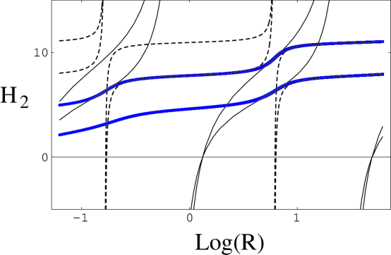
Figure 1: The running coupling for the $n=2$ singular potential. The solid lines are given by Eq. (8) and the dashed lines are given by Eq. (9). The bold lines are a numerical solution of Eq. (7).

The three-body problem with short-range interactions is known to be equivalent, in the ultraviolet regime, to the $1/r^{2}$ potential [6]. The role of the interparticle distance $r$ is played in the three-body problem by a collective coordinate that vanishes when the three particles occupy the same point in space, and the analogue of the three-body force is the short-distance potential. Since renormalization depends only on the short-distance behavior of the theory, it is not surprising that the renormalization of the three-body problem requires the presence of a three-body force [7]. Using momentum-cutoff regularization the running of the three-body force was found to follow Eq. (8) very closely, even where this formula predicts a pole. Evidently, for values of ${\cal R}$ where Eq. (9) takes over in the $1/r^{2}$ problem, the three-body force continues to follow Eq. (8) and seems to reach arbitrarily high values. Also, no evidence of multiple branches was found in the three-body problem. These discrepancies between the three-body and the $1/r^{2}$ problem may be due to the fact that not all aspects of the renomalization-group flow are universal, in the sense of being independent of the particular regulator used.

3.3 The Full Solution

In the case $n=2$, the Schrödinger equation can be solved exactly for all energies. The solution is

$$u(x;\eta)=\sqrt{x}\left[\exp{(i\alpha)}J_{i\nu}(\eta x)+\exp{(-i\alpha)}J_{-i\nu}(\eta x)\right]$$ (10)

where the $J_{\pm i\nu}$ are Bessel functions, and $\alpha$ is to be fixed by a boundary condition. For small $x$ we find

$$u(x;\eta)=\sqrt{x}\cos{\left(\nu\log{(x\eta/2)}+\alpha-{\rm Im}\log\Gamma(1+i\nu)\right)}.$$ (11)

Matching to Eq. (6) gives

$$\phi_{2}=\alpha+\nu\log\eta/2-{\rm Im}\log\Gamma(1+i\nu).$$ (12)

Since $\phi_{2}$ is, by construction, energy independent, $\alpha$ is energy dependent.

We can now look for solutions with $\eta=i\kappa$ which fall off exponentially at large $x$. It follows from Eq. (10) that

$$u(x;\kappa)\rightarrow\frac{1}{2}\exp{(i{\pi\over 4})}\cos(\alpha+i\frac{\nu\pi}{2})\exp{(\kappa x)}+C\exp{(-\kappa x)}$$ (13)

where $C$ is an energy-dependent coefficient. The bound-state solutions then correspond to $\alpha(\eta)=(m+1/2)\pi-i\nu\pi/2$, with $m$ an integer. Comparing with Eq. (12) gives the bound-state spectrum

$$E_{m}=-{2\over{M{r_{0}^{2}}}}\exp{\left(2{{{\phi_{2}+{\rm Im}\log\Gamma(1+i\nu)-(m+1/2)\pi}}\over\nu}\right)}.$$ (14)

Once $\phi_{2}$ is fixed by a single bound-state energy, all other energies are predicted [2]. Adjacent bound-state energies are related by

$${{\kappa_{m+1}}\over{\kappa_{m}}}=\exp{(-{\pi\over\nu})}.$$ (15)

Hence we see that the periodicity in the running coupling $H_{2}({\cal R})$ is associated with the accumulation or dissipation of bound states near the origin.

One can also fix $\phi_{2}$ to a scattering observable, like the scattering length or the phase shift at a given energy. Unfortunately, as for the Coulomb potential, the $n=2,3$ singular potentials suffer infrared problems at low energies, and therefore scattering lengths can be defined only if an infrared cutoff is imposed [3].

4 Pure Singular Potentials: $n\geq 3$

4.1 The $k=0$ Solution

The exact zero-energy solution for $n\geq 3$ is well known [3]. Defining $z=\sqrt{\lambda_{L}}x^{1-n/2}/|1-n/2|$ and $\phi(z)=u(x;0)/\sqrt{x}$, for $x>{\cal R}$ Eq. (3) becomes an ordinary Bessel equation:

$$\phi^{\prime\prime}(z)+\frac{1}{z}\phi^{\prime}(z)+\left(1-\frac{1}{(n-2)^{2}z^{2}}\right)\phi(z)=0.$$ (16)

The solution is

$$u(x;0)=\sqrt{x}\left[A_{n}J_{1/(n-2)}\left(\frac{\sqrt{\lambda_{L}}}{1-n/2}x^{1-n/2}\right)+B_{n}J_{-1/(n-2)}\left(\frac{\sqrt{\lambda_{L}}}{1-n/2}x^{1-n/2}\right)\right],$$ (17)

which is a linear combination of Bessel functions. For small $x$ we can write

$$u(x;0)={x^{{n/4}}}\cos\left({\sqrt{\lambda_{L}}\over{{n/2}-1}}{x}^{1-{n/2}}+\phi_{n}\right)\;\left[1\;+\;{\cal O}(x^{n/2-1})\right],$$ (18)

where we have set the constant prefactor to unity and

$$\phi_{n}=-{{n\pi}\over 4}{1\over{(n-2})}+i\log{\left(1+{{B_{n}}\over{A_{n}}}\exp{\left(-{{i\pi}\over{(n-2)}}\right)}\right)}.$$ (19)

This solution exhibits precisely the same pathologies as Eq. (6).

4.2 Matching to the Square Well

We proceed as in the case $n=2$. Again we have a square well in the interior region. Matching logarithmic derivatives at the boundary $x={\cal R}$ gives

$$\sqrt{\lambda_{S}}\cot{\sqrt{\lambda_{S}}{\cal R}}={n\over{4{\cal R}}}-\left({{\lambda_{L}}\over{{\cal R}^{n}}}\right)^{1/2}\tan\left({\sqrt{\lambda_{L}}\over{{n/2}-1}}{\cal R}^{1-{n/2}}+\phi_{n}\right)$$ (20)

where we have neglected ${\cal O}({\cal R}^{n/2-1})$ corrections to the wavefunction at $x>{\cal R}$. The phase $\phi_{n}$ is physical and can be traded for the scattering length (for $n>3$), as will be seen below. If we vary ${\cal R}$ and $\lambda_{S}({\cal R})$ as given here, the phase $\phi_{n}$ will not be affected. We proceed as we did before in the $n=2$ case and find, in the regions where the right-hand side of Eq. (20) is large

$$H_{n}({\cal R})={m\pi}\left\{1-\frac{1}{1-n/4+\sqrt{\lambda_{L}}{\cal R}^{1-n/2}\tan\left(\frac{2\sqrt{\lambda_{L}}}{n-2}{\cal R}^{1-n/2}+\phi_{n}\right)}\right\}.$$ (21)

In the other regime, where the right-hand side is close to a zero, we have

$$H_{n}({\cal R})={(m+{1\over 2})\pi}-{1\over{(m+{1\over 2})\pi}}\left(n/4-\sqrt{\lambda_{L}}{\cal R}^{1-n/2}\tan\left(\frac{2\sqrt{\lambda_{L}}}{n-2}{\cal R}^{1-n/2}+\phi_{n}\right)\right).$$ (22)

A numerical solution of Eq. (20) in the case $n=4$ shows that the approximate solutions Eqs. (21,22) are very good within their ranges of validity. The expression in Eq. (22) interpolates between two successive branches of Eq. (21) (see Fig. 2).

The scattering length can be found from the zero-energy wavefunction for $n\geq 4$ [14]. For instance, we find the $n=4$ scattering length

$$a_{4}={r_{0}}\sqrt{\lambda_{L}}\tan\phi_{4}.$$ (23)

It is evident that $a_{4}$ determines the phase $\phi_{4}$.

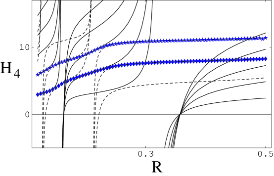
Figure 2: The running coupling for the $n=4$ singular potential. The solid line is given by Eq. (21) and the dashed line is given by Eq. (22). The triangles and stars are extracted from numerically solving the Schrödinger equation and coincide exactly with the numerical solution of Eq. (20),

5 The WKB Approximation

There is an important shortcoming in what we have done so far. Defining zero-energy scattering is not sufficient to guarantee correct renormalization. We want physics at all energies $\eta\hskip 1.99997pt\raisebox{2.15277pt}{$<$}\raisebox{-3.00003pt}{$\sim$}\hskip 1.99997pt1$ to be cutoff independent. It is clear that the above procedure could in principle be repeated at each energy by allowing energy dependence in $\lambda_{S}$. Fixing $\phi_{n}$ at one energy and then predicting other energies will only result if the scale of this energy dependence is much slower than $1/2Mr_{0}^{2}$, so that, to some accuracy, $\lambda_{S}$ can be taken to be energy independent. Otherwise, an infinite number of parameters (the strength of arbitrarily-many-derivative contact interactions) would have to be known in order to have predictive power. This shortcoming can be removed using the WKB approximation. We can also consider the more general case, $f(x)\neq 1$.

5.1 The WKB Criteria

We now keep $f(x)$ arbitrary and consider the region $x>{\cal R}$ in the limit ${x}\rightarrow 0$. A particularly well-suited approximation in this limit is the WKB approximation, which is valid when the wavelength $\lambda$ is small compared to the characteristic distance over which the potential varies appreciably. That is

$${1\over{2\pi}}\bigl{|}{{d\lambda}\over{dr}}\bigr{|}=|{{d}\over{dr}}[2M(E-V(r))]^{-1/2}|\ll 1,$$ (24)

which translates into the constraint

$${2\over n}\sqrt{\lambda_{L}f(x)}\gg x^{n/2-1}$$ (25)

in the small-$x$ region. Clearly this condition is satisfied for all $n>2$ as $x\rightarrow 0$. In the marginal case $n=2$ this condition is satisfied only for a sufficiently strong potential. Therefore the WKB criterion parallels the general argument given above based on the boundedness of the Hamiltonian. The general WKB solution [12] is

$$u(x;\eta)=\left(\eta^{2}+{{{\lambda_{L}}{f(x)}}\over{x^{n}}}\right)^{-1/4}\cos\left(\int_{x_{0}}^{x}dx^{\prime}\left(\eta^{2}+{{{\lambda_{L}}{f(x^{\prime})}}\over{x^{\prime n}}}\right)^{1/2}\right)$$ (26)

where $x_{0}$ is a constant of integration. For $V\gg E$ this reduces to

$$u(x;0)=x^{n/4}f^{-1/4}(x)\cos\left(\sqrt{\lambda_{L}}\int_{x_{0}}^{x}dx^{\prime}x^{\prime-n/2}f^{1/2}(x^{\prime})\right).$$ (27)

In the limit ${\cal R}<x\ll 1$, we can set $f(x)=1$ (keep the leading term in a power series in $x$). We then recover, for $n>2$,

$$u(x;0)=x^{n/4}\cos\left(\frac{\sqrt{\lambda_{L}}}{n/2-1}x^{1-n/2}+\phi_{n}\right)$$ (28)

where $\phi_{n}={-{\sqrt{\lambda_{L}}{x_{0}}^{-n/2+1}}/{(1-n/2)}}$. The case $n=2$ is also recovered if one takes $\lambda_{L}\rightarrow\lambda_{L}-1/4$. Therefore, we expect our conclusions about the renormalization of the singular potentials to be valid for the more general case $f(x)\neq 1$.

5.2 The Leading Energy Dependence

We now show that the zero-energy solution is in fact sufficient to remove cutoff dependence at all other low energies. The crucial point is that, in the intermediate region ${\cal R}<x\ll 1$, for the energies of interest, the potential energy is much larger than the total energy, and we recover the zero-energy case. This can be made more precise using WKB again [2]. We write the wavefunction for any $x\geq{\cal R}$ as

$$u(x;\eta)=A(x;\eta)u(x;0).$$ (29)

Then $A(x;\eta)$ obeys

$$\frac{d^{2}A(x)}{dx^{2}}+2\frac{d\ln u(x;0)}{dx}\frac{dA(x)}{dx}+\eta^{2}A(x)=0$$ (30)

which depends only on the zero energy wavefunction. Now, since for ${\cal R}<x\ll 1$,

$$\left|\frac{d\ln u(x;0)}{dx}\right|\gg 1,$$ (31)

$A(x)$ can be written

$$A(x)=A_{(0)}(x)+A_{(1)}(x)+\ldots,$$ (32)

where

$$\frac{dA_{(0)}}{dx}=0;\qquad\frac{dA_{(1)}}{dx}=-{1\over 2}\frac{u(x;0)}{u^{\prime}(x;0)}\eta^{2}A_{(0)};\qquad\ldots$$ (33)

We then find the leading energy corrections

$$A(x;\eta)=A_{(0)}\left\{1-\frac{\eta^{2}}{2}\int_{0}^{x}dx^{\prime}\frac{u(x^{\prime};0)}{u^{\prime}(x^{\prime};0)}+\ldots\right\}$$ (34)

We see that, in the intermediate region, the energy dependence of the wavefunction (29) is determined by the zero-energy wavefunction $u(x;0)$. If the phase of $u(x;0)$ has been fixed, the phase of $u(x;\eta)$ is fixed, and scattering observables can be predicted at low energies.

5.3 Error Estimates

The fact remains that our arguments are all at short distances where the WKB approximation is valid. This is, of course, the opposite of the EFT limit which interests us. One may wonder whether cutoff effects can be amplified when propagating the wavefunction from short to long distances. We will see now that this cannot occur and in turn find an estimate of the cutoff error associated with the scattering phase shift. Usually, in perturbative EFT, the error is a power law in ${\cal R}$. Here we will find a more complicated functional dependence.

By adjusting $H_{n}({\cal R})$ as in Eqs. (21,22) we guarantee that two zero-energy solutions $u_{\cal R}(x;0)$, $u_{\cal R^{\prime}}(x;0)$ corresponding to two different cutoffs ${{\cal R}},{\cal R}^{\prime}\ll 1\sim 1/\eta$ are identical. At finite values of $\eta$, solutions obtained with different cutoffs will no longer be equal, but their difference can be easily estimated. Taking ${\cal R^{\prime}}<{\cal R}$, the Schrödinger equations satisfied by $u_{\cal R}(x;\eta)$ and $u_{\cal R^{\prime}}(x;\eta)$ are the same in the $x>{\cal R}$ region so their Wronskian,

$$W[u_{\cal R},u_{\cal R^{\prime}}](x;\eta)=u_{\cal R}(x;\eta)u_{\cal R^{\prime}}^{\prime}(x;\eta)-u_{\cal R}^{\prime}(x;\eta)u_{\cal R^{\prime}}(x;\eta)$$ (35)

is independent of $x$. At large distances ($r\gg(\lambda_{L}/k^{2})^{(1/n)}$), where the solutions are plane waves, $W[u_{\cal R},u_{\cal R^{\prime}}]$ is related to the phase shifts $\delta_{\cal R},\delta_{\cal R^{\prime}}$ obtained with the cutoffs ${\cal R}$ and ${\cal R^{\prime}}$ by

$$W[u_{\cal R},u_{\cal R^{\prime}}](r\gg(\lambda_{L}/k^{2})^{(1/n)};\eta)=A_{\cal R}A_{\cal R^{\prime}}\eta\sin(\delta_{\cal R}-\delta_{\cal R^{\prime}}),$$ (36)

where $A_{\cal R},A_{\cal R^{\prime}}$ are the amplitudes at large distances. These prefactors are easily estimated from the general WKB solution, Eq. (26), in the region $r\gg(\lambda_{L}/k^{2})^{(1/n)}$, where the WKB solution maps to the asymptotic plane-wave solution (see Footnote 9). We find $A_{\cal R}\,,A_{\cal R^{\prime}}\sim\eta^{-1/2}$.

On the other hand, at the cutoff distance $x={\cal R}$, $W[u_{\cal R},u_{\cal R^{\prime}}]$ is estimated using our WKB formula, Eq. (34). We find

$$W[u_{\cal R},u_{\cal R^{\prime}}]({\cal R};\eta)=W[u_{\cal R},u_{\cal R^{\prime}}]({\cal R};0)-{{\eta^{2}}\over 2}{\cal E}({\cal R};0)+\ldots$$ (37)

where

$$W[u_{\cal R},u_{\cal R^{\prime}}]({\cal R};0)=u_{\cal R}({\cal R};0)u_{\cal R^{\prime}}({\cal R};0)\left[\frac{u_{\cal R^{\prime}}^{\prime}({\cal R};0)}{u_{\cal R^{\prime}}({\cal R};0)}-\frac{u_{\cal R}^{\prime}({\cal R};0)}{u_{\cal R}({\cal R};0)}+{\cal O}\left({\cal R}^{n/2-1}{\frac{u_{\cal R}^{\prime}({\cal R})}{u_{\cal R}({\cal R})}}\right)\right]$$ (38)

and

$${\cal E}({\cal R};0) \equiv u_{\cal R}({\cal R};0)u_{\cal R^{\prime}}({\cal R};0)\left[\frac{u_{\cal R^{\prime}}({\cal R};0)}{u_{\cal R^{\prime}}^{\prime}({\cal R};0)}-\frac{u_{\cal R}({\cal R};0)}{u_{\cal R}^{\prime}({\cal R};0)}+{\cal O}\left({\cal R}^{n/2-1}{\frac{u_{\cal R}({\cal R})}{u_{\cal R}^{\prime}({\cal R})}}\right)\right]$$ (39)

$$+ W[u_{\cal R},u_{\cal R^{\prime}}]({\cal R};0){\int_{0}^{{\cal R}}}dx^{\prime}\left[\frac{u_{\cal R^{\prime}}(x^{\prime};0)}{u_{\cal R^{\prime}}^{\prime}(x^{\prime};0)}+\frac{u_{\cal R}(x^{\prime};0)}{u_{\cal R}^{\prime}(x^{\prime};0)}+{\cal O}\left({x^{\prime}}^{n/2-1}{\frac{u_{\cal R}(x^{\prime})}{u_{\cal R}^{\prime}(x^{\prime})}}\right)\right].$$

We have included the error due to keeping only the leading zero-energy wavefunction in Eq. (18). Recall that we choose our fitting procedure to be energy independent, for example, by comparing the zero-energy wavefunction to the scattering length. It then follows that $W[u_{\cal R},u_{\cal R^{\prime}}]({\cal R};0)=0$, by construction, for the full wavefunction, and from Eq. (38) we have

$$\frac{u_{\cal R^{\prime}}^{\prime}({\cal R};0)}{u_{\cal R^{\prime}}({\cal R};0)}-\frac{u_{\cal R}^{\prime}({\cal R};0)}{u_{\cal R}({\cal R};0)}={\cal O}\left({\cal R}^{n/2-1}{\frac{u_{\cal R}^{\prime}({\cal R})}{u_{\cal R}({\cal R})}}\right).$$ (40)

Using these constraints it is straightforward to find

$${\cal E}({\cal R};0)={\cal O}\left({\cal R}^{n/2-1}\frac{{(u_{\cal R}({\cal R}))^{3}}}{u_{\cal R}^{\prime}({\cal R})}\right).$$ (41)

If we assume that all oscillating functions of ${\cal R}$ are of order unity for values of ${\cal R}$ at which we fit observables, then ${\cal E}({\cal R};0)={\cal O}({\cal R}^{3n/2-1})$, which is small for all $n\geq 2$. Matching the Wronskians at large ($r\gg(\lambda_{L}/k^{2})^{(1/n)}$) and short ($x={\cal R}$) distances then yields an estimate for the error in the phase shift:

$$\delta_{\cal R}-\delta_{\cal R^{\prime}}\sim\eta^{2}\ \ {\cal E}({\cal R};0)$$ (42)

where ${\cal E}({\cal R};0)$ is a function of $\cal R$ whose complicated parametric cutoff dependence is given by Eq. (41). This shows that the renormalization procedure described here produces cutoff independent phase shifts, accurate up to order $\eta^{2}\ {\cal E}({\cal R};0)$.

6 The Weak Coupling Limit

It might seem odd that the explicit dependence on the coupling constant is nonanalytic in the formula for the $n=4$ scattering length, Eq. (23). Naively it would appear that nonperturbative effects are important at arbitrarily weak coupling.

However, we know that this cannot be the case, since for weak coupling the scattering length should go smoothly to its square-well value. We would expect a perturbative description in the singular potential to be valid when the potential energy, $-{\lambda_{L}}{x^{-n}}$, is much smaller than the kinetic energy, ${x^{-2}}$. This leads to the condition

$$r\gg{r_{0}}\lambda_{L}^{1\over{n-2}},\quad{\rm or}\qquad k\ll{r_{0}^{-1}}\lambda_{L}^{-{1\over{n-2}}}.$$ (43)

In effect, taking $\phi_{4}$ from Eq. (20) we find, for $\lambda_{L}/{\cal R}^{2}\ll 1$,

$$\frac{a_{4}}{R}=\left(1-\frac{\tan({\sqrt{{\lambda_{S}}}}\,{\cal R})}{{\sqrt{{\lambda_{S}}}{\cal R}}}\right)-\frac{1}{3}\left(1+\frac{\tan({\sqrt{{\lambda_{S}}}}\,{\cal R})}{{\sqrt{{\lambda_{S}}}{\cal R}}}+\left(\frac{\tan({\sqrt{{\lambda_{S}}}}\,{\cal R})}{{\sqrt{{\lambda_{S}}}{\cal R}}}\right)^{2}\right){{\lambda_{L}}\over{{\cal R}^{2}}}+{{\cal O}({{{\lambda_{L}}^{2}}\over{{\cal R}^{4}}})}.$$ (44)

Leading order reproduces the square-well scattering length and the corrections are analytic in $\lambda_{L}$. Hence, there is, in fact, no nonanalyticity near zero coupling in the presence of the square well.

Of course, if the cutoff $\cal R$ is taken at values where the oscillatory behavior of the wavefunction has set in, ${\cal R}\hskip 1.99997pt\raisebox{2.15277pt}{$<$}\raisebox{-3.00003pt}{$\sim$}\hskip 1.99997pt\lambda_{L}^{1\over{n-2}}$, then there is no sense in which perturbation theory in $\lambda_{L}$ can capture the true behavior of the wavefunction. This is made clear in Fig.  3 where several orders in a perturbative expansion of the $n=4$ singular-potential wavefunction are plotted against the exact singular-potential wavefunction in the short-distance region.

Figure 3: The exact zero-energy wavefunction (solid line) at small $r$ compared with the wavefunction obtained in perturbation theory to leading order (small dashes), next-to-leading order (medium dashes), and next-to-next-to-leading order (large dashes).

7 Numerics

In this section we analyze the $1/r^{4}$ potential numerically. For simplicity, we take $2M={r_{0}}=1$; therefore, $x=r$ and $\eta=k=\sqrt{2E}$. The long-distance potential is then completely determined by $\lambda_{L}$ which we take to be unity. We consider the “natural case”, which is characterized by $a_{4}\sim(\lambda_{L})^{1/2}$, and the “unnatural case”, which is characterized by $a_{4}\gg(\lambda_{L})^{1/2}$.

In Fig. 4 we show phase shifts $\delta(k)$ in a natural case ($\delta(0.1)=0.1$ and $\phi_{4}=-101.298$) for various cutoffs. We see that, as anticipated, the low-energy phases are to a good approximation cutoff independent; cutoff dependence becomes more pronounced as the cutoff radius and the energy are increased. In the same figure we also plot the error analysis: the (log of the) errors $|\Delta\delta(k)|=\delta_{R}-\delta_{R^{\prime}}$ as a function of (the log of the) energy for various pairs of cutoffs. We find that the errors scale as $k^{2}$, as expected on the basis of Eq. (42). In Fig. 5 we show the corresponding results in an “unnatural” case ($\delta(0.1)=\pi/3$ and $\phi_{4}=-98.954$). Again we find that the errors scale as $k^{2}$.

Figure 4: Left: phase shifts $\delta$ vs. energy in the case of a natural scattering length for $n=4$. Various cutoffs are given with the square well tuned to give the same scattering length. The cutoffs are $R=.01$ (dots), $R=.02$ (triangles), $R=.04$ (squares), $R=.08$ (stars), $R=.16$ (diamonds). Right: logarithm of the errors $|\Delta\delta(k)|=\delta_{R}-\delta_{R^{\prime}}$ as a function of the logarithm of the energy for $n=4$. The pairs of cutoffs $(R,R^{\prime})$ are: $(.16,.08)$ (diamonds), $(.08,.04,)$ (stars), $(.04,.02,)$ (squares), $(.02,.01,)$ (triangles).

Figure 5: Same as Fig. 4 for an unnatural scattering length.

8 Conclusion

We have reconsidered singular potentials of the form $1/r^{n}$ with $n\geq 2$ from the viewpoint of modern renormalization theory. We have shown that the well-known pathologies near the origin are cured by a square-well counterterm which represents the effect of unknown short-distance physics. The renormalization-group evolution of this counterterm has periodic behavior. The counterterm is not determined uniquely at any given cutoff due to the infinite number of branches of the renormalization-group flow, and one is allowed to freely jump from branch to branch at will without causing any change in the low-energy phase shifts (up to ${\cal O}(k^{2})$ corrections).

The dependence of the number of bound states on the choice of branch is complex. Arguments similar to the one leading to Eq. (14) are valid for a generic singular potential as long as (i) the binding energy is much smaller that $\lambda_{S}/(2Mr_{0}^{2})$ (in order that the binding energy can be disregarded in the left-hand side of Eq. (20)) and (ii) the binding energy is much larger than $\lambda_{L}/(2Mr_{0}^{2})$ (so the fact that $f(r/r_{0})\neq 1$ is unconsequential). The resulting spectrum shows a power-law distribution that is given by the WKB estimate [14]. We see now that as ${\cal R}\rightarrow 0$ and $\lambda_{S}({\cal R})\rightarrow\infty$ the region of validity of the calculation sketched above grows and more and more bound states are created. If, in addition to keeping the phase shifts cutoff independent, one also demands that the number of bound states also be fixed, the value of the counterterm $\lambda_{S}$ jumps down a branch at every cycle. We are then left with a periodic, limit-cycle behavior for the renormalization-group flow. This is a unique situation in field theory/critical phenomena, where the standard behavior corresponds to counterterms approaching either zero (asymptotic freedom) or infinity as the momentum cutoff goes to infinity  [8].

Naively it appears that the singular potentials have a nonanalytic dependence on the coupling parameter even at weak coupling. This would negate a perturbative description at weak coupling, a conclusion which must be incorrect. One might imagine some as yet experimentally invisible light particle which interacts at long distances via a singular potential (e.g. an axion). If the behavior of the wavefunction were such that there is a branch point at the origin of the coupling-constant plane, then nonperturbative effects would persist even for couplings of gravitational strength. We have seen that this nonanalyticity is an artifact which is removed by short-distance physics encoded by the square well.

Renormalization renders low-energy phase shifts cutoff independent up to ${\cal O}(k^{2})$ corrections. The cutoff dependence of these errors is not generally a power law as one expects in Wilsonian EFT. The renormalization-group flow introduces complicated oscillatory behavior in the corrections, which nonetheless is small for judiciously chosen cutoffs. Our theoretical expectations of the error have been confirmed numerically. We expect that the methods developed in this paper will prove useful to those interested in the cornucopia of physical systems whose long-distance behavior is governed by singular potentials.

Acknowledgments

We thank David Kaplan, Hans Hammer and Martin Savage for valuable conversations and Sid Coon for bringing Ref. [14] to our attention. UvK thanks the Nuclear Theory Group and the Institute for Nuclear Theory at the University of Washington for hospitality, and RIKEN, Brookhaven National Laboratory and the U.S. Department of Energy [DE-AC02-98CH10886] for providing the facilities essential for the completion of this work. This research was supported in part by the DOE grants DE-FG03-97ER41014 (SRB) and DOE-ER-40561 (PFB), and by NSF grant PHY 94-20470 (UvK). LC and JMc are grateful to the University of Washington REU program of the NSF for support.

References

- [1] M. Plesset, Phys. Rev. 41, 278 (1932).
- [2] K.M. Case, Phys. Rev. 80, 797 (1950).
- [3] For a comprehensive review, see W.M. Frank, D.J. Land and R.M. Spector, Rev. Mod. Phys. 43, 36 (1971).
- [4] For reviews, see D.B. Kaplan, nucl-th/9506035; P. Lepage, nucl-th/9706029.
- [5] H.E. Camblong et. al., Phys. Rev. Lett. 85, 1590 (2000), hep-th/0003014; hep-th/0003255; hep-th/0003267.
- [6] V.N. Efimov, Sov. J. Nucl. Phys. 12, 589 (1971).
- [7] P.F. Bedaque, H.-W. Hammer, and U. van Kolck, Nucl. Phys. A646, 444 (1999), nucl-th/9811046; P.F. Bedaque, H.-W. Hammer, and U. van Kolck, Phys. Rev. Lett. 82, 463 (1999), nucl-th/9809025.
- [8] K. Wilson, A Limit Cycle for Three-Body Short Range Forces, talk presented at the Institute for Nuclear Theory, University of Washington, 2000.
- [9] J-M. Levy-Leblond, Phys. Rev. 153, 1 (1967); O.H. Crawford, Proc. Phys. Soc. 91, 279 (1967).
- [10] See, for instance, U. van Kolck, Prog. Part. Nucl. Phys. 43, 409 (1999); S.R. Beane et. al., nucl-th/0008064.
- [11] E. Vogt and H. Wannier, Phys. Rev. 95, 1190 (1954).
- [12] L.D. Landau and E.M. Lifshitz, Quantum Mechanics, (Pergamon Press, London, 1965).
- [13] See, for instance, C. Itzykson and J-B. Zuber, Quantum Field Theory, (McGraw-Hill, New York, 1980).
- [14] A.M. Perelomov and V.S. Popov, Teor. Mat. Fiz. 4, 664 (1970).