Decoherence in a superconducting ring

Abstract

A superconducting ring has different sectors of states corresponding to different values of the trapped magnetic flux; this multitude of states can be used for quantum information storage. If a current supporting a nonzero flux is set up in the ring, fluctuations of electromagnetic field will be able to “detect” that current and thus cause a loss of quantum coherence. We estimate the decoherence exponent for a ring of a round type-II wire and find that it contains a macroscopic suppression factor $(\delta/R_{1})^{2}$, where $R_{1}$ is the radius of the wire, and $\delta$ is the London penetration depth. We present some encouraging numerical estimates based on this result.

I Introduction and results

A superconducting ring is a good candidate for macroscopic quantum memory [1]. Its ability to store quantum information stems from the complicated “vacuum structure”, viz. the presence of different sectors of states corresponding to different values of magnetic flux through the ring.

It is easy to suppress spontaneous transitions between these different sectors by making the ring sufficiently thick [1]. In the absence of such transitions, the main mechanism by which quantum information stored in the ring deteriorates is decoherence, i.e. a decrease, in time, of matrix elements between states with different values of the flux. Decoherence is due to interaction of the macroscopic variable, in our case the supercurrent in the ring, with the “environment” comprised by local degrees of freedom—fluctuations of the electromagnetic field.

The supercurrent density required to support a single flux quantum through a macroscopic ring is very small. This makes that state locally almost indistinguishable from the state with no flux at all. Based on this observation, we have suggested [1] that in this case decoherence may not be as strong as it is generally believed to be for macroscopic systems. The purpose of the present paper is to discuss decoherence in the ring quantitatively.

In general, the environment starts out in an arbitrary initial state with some density matrix $\rho_{0}$. Two different values of the macroscopic variable give rise to two different histories of the environment, which are represented by evolution operators $U_{1}(t)$ and $U_{2}(t)$. We define the amount of coherence (at time $t$) between these two histories as the “overlap”

$${\cal C}(t)=\mbox{\rm Tr}[U_{1}(t)\rho_{0}U_{2}^{\dagger}(t)]\;.$$ (1)

Next, we define a decoherence exponent $D(t)$ by

$$\exp[-D(t)]=\left|{\cal C}(t)\right|^{2}\;.$$ (2)

For an environment comprised by linear oscillators, which in addition interact linearly with the macroscopic variable, decoherence had been widely discussed in connection with macroscopic tunneling [2, 3]. That problem is similar but not identical to ours: in quantum memory tunneling is suppressed. Indeed, our problem is more analogous to the “error-free” case of ref. [4]; however, we will be able to supply definite values for all of our parameters.

In principle, the linear approximation can break down at large times even for weakly nonlinear environments. In addition, whatever we designate as the environment will interact with a still larger system and will loose energy to that system at some characteristic dissipation rate. For example, in our case, the electromagnetic field can be absorbed on the surface of the superconductor, as well as on the surfaces of any surrounding objects. In such cases, the evolution of the environment can no longer be represented by unitary operators.

It is certainly of interest to understand how nonlinearity and dissipation in the environment affect quantum coherence in the original system. However, for our present purposes the linear approximation will be sufficient. A mechanism for decoherence exists already at the linear level [3]. Dissipation will only be discussed phenomenologically, to make sure that it does not significantly alter the evolution of the oscillators at relevant times.

Specifically, we consider the following problem. Suppose at the initial time $t=0$ a supercurrent has been set up in the ring but the electromagnetic field is still in the thermal state corresponding to zero current, with a Gibbs distribution $w_{m}$ of probabilities for the energy eigenstates $|m\rangle$. Because the field is displaced from its true equilibrium (corresponding to a nonzero average magnetic field), it will oscillate. Consider two oscillation histories, corresponding to two different values of the current (one of which may be zero), and call their evolution operators $U_{1}(t)$ and $U_{2}(t)$. The decoherence exponent in this case will be determined by

$$\exp[-D(t)]=\sum_{m}\left|\langle m|U_{2}^{\dagger}U_{1}|m\rangle\right|^{2}w_{m}\;.$$ (3)

We describe a calculation of $D(t)$ below.

The problem just posed is admittedly somewhat artificial. Imagine that we switch from the state with no flux (and no current) to the state with unit flux by dragging a single flux line through the bulk of the superconductor. There is no reason to expect that the current will equilibrate first, and the field next, as in our model problem. Nevertheless, we think that it is good to know the answer to this model problem before turning to more realistic setups.

The answer is this. Consider a circular ring of radius $R_{0}$ made out of a London-type superconducting round wire of radius $R_{1}$, in the limit

$$\delta\ll R_{1}\ll R_{0}\;,$$ (4)

where $\delta$ is the London penetration depth. We find that at intermediate times $R_{1}/c\ll t\ll R_{0}/c$ ($c$ is the speed of light), the exponent $D(t)$ grows as $t$ for $t\ll\hbar/k_{B}T$ and as $t^{2}$ for $t\gg\hbar/k_{B}T$, up to some logarithms. At large times, $t\gg R_{0}/c$, the exponent saturates at a certain limiting value, for which we obtain the following estimate:

$$D_{\rm lim}\sim\frac{f(u)}{16\alpha_{\rm EM}\ln^{4}(R_{0}/R_{1})}\left(\frac{\pi c}{R_{0}\omega_{\rm min}}\right)\left(\frac{\delta}{R_{1}}\right)^{2}\;,$$ (5)

where $\alpha_{\rm EM}$ is the fine-structure constant, and $u=k_{B}T/\hbar\omega_{\rm min}$ with $\omega_{\rm min}\sim c/R_{0}$; $f(u)=1$ for small $u$, and $f(u)=u$ for large $u$.

The main result is the macroscopic suppression factor $(\delta/R_{1})^{2}$ in (5). Taking for estimates $\delta\sim 10^{-5}$ cm, $R_{0}=1$ cm, $R_{1}=1$ mm, $\omega_{\rm min}=\pi c/R_{0}\sim 10^{11}$ s^-1, and replacing the logarithm (which controls logarithmic accuracy) with unity, we obtain $x\sim T/({\rm 1~{}K})$ and $D_{\rm lim}\sim 10^{-7}f(x)$.

These results apply not only to a ring made out of a solid superconductor, but also to a ring coated with a superconducting film, as long as the thickness of the film is much larger than the London depth $\delta$. Similar calculations can be done for any type of persistent circular current, of which a supercurrent in a macroscopic ring is but one limiting case. The opposite limit is a circular current in a single atom—e.g. a circular Rydberg state [5], which has already been proposed as a basis for quantum computation [6]. It would be interesting to do the calculation for that case and see how the decoherence rate changes as the current loop becomes microscopic.

We now outline the main steps leading to estimate (5).

II The oscillator Hamiltonian

We will only consider decoherence at times

$$t\gg R_{1}/c\;,$$ (6)

when, as we will see, the main contribution to the decoherence exponent comes from electromagnetic modes with low frequencies:

$$\omega\ll c/R_{1}\;.$$ (7)

For such modes, the response of a superconductor of the London type (the only type we consider) is determined, to a good accuracy, by the London penetration depth $\delta$.

To count the oscillator modes, we enclose the ring in a large normalization sphere of radius ${\cal R}\gg R_{0}$, centered at the center of the ring. We define a system of spherical coordinates $(r,\theta,\phi)$, with angle $\theta$ measured form the axis of the ring’s rotational symmetry.

Only the azimuthal component of the vector potential, indeed only the $\phi$-independent modes of it, interact with the current. For these modes, the vector potential takes the form

$$\mbox{\bf A}(r,\theta,\phi;t)=\mbox{\bf e}_{\phi}(\phi)A(r,\theta;t)\;,$$ (8)

where $\mbox{\bf e}_{\phi}$ is the azimuthal unit vector. Then,

$$\nabla^{2}\mbox{\bf A}=\mbox{\bf e}_{\phi}\left(\nabla^{2}-\frac{1}{r^{2}\sin^{2}\theta}\right)A\;,$$ (9)

and the wave equation for ${\bf A}$ takes the form

$$\ddot{A}-\nabla^{2}A+\left[\frac{1}{r^{2}\sin^{2}\theta}+V(r,\theta)\right]A=\frac{4\pi}{c}j\;.$$ (10)

Here $j$ is the constant (in time) supercurrent density, and $V(r,\theta)$ is the “potential” that represents the Meissner effect: inside the superconductor

$$V(r,\theta)=1/\delta^{2}\;,$$ (11)

while outside the superconductor both $j$ and $V$ are zero.

The equation of motion (10) can be obtained, after substitution (8), from the effective Hamiltonian

$$H=\int d^{3}x\left(\frac{1}{8\pi c^{2}}\dot{\mbox{\bf A}}^{2}+\frac{1}{8\pi}\mbox{\bf B}^{2}+\frac{V}{8\pi}{\mbox{\bf A}}^{2}-\frac{1}{c}\mbox{\bf A}\mbox{\bf j}\right)\;,$$ (12)

where $\mbox{\bf B}=\nabla\times\mbox{\bf A}$ is the magnetic field, and $\mbox{\bf j}=\mbox{\bf e}_{\phi}j$. Such Hamiltonian formulation neglects any dissipation (absorption) of the electromagnetic field. This approximation is justified in Appendix A. We stress again that decoherence we calculate in this paper is not due to any such dissipation, but is a result of a “measurement” of the supercurrent, performed by fluctuations of the electromagnetic field.

Now, expand the field $A$ in a complete set of modes $f_{n}(r,\theta)$:

$$A(r,\theta;t)=\sum_{n}f_{n}(r,\theta)X_{n}(t)\;.$$ (13)

This expansion defines a set of oscillator coordinates $X_{n}$. The modes $f_{n}$ satisfy the following equation:

$$\left[-\nabla^{2}+\frac{1}{r^{2}\sin^{2}\theta}+V(r,\theta)\right]f_{n}=\frac{\omega_{n}^{2}}{c^{2}}f_{n}\;,$$ (14)

where $\omega_{n}$ are real eigenfrequencies, together with the continuity conditions at the surface of the superconductor and some boundary condition at the boundary of the normalization volume. They are normalized in that volume by

$$\int d^{3}xf_{n}(r,\theta)f_{n^{\prime}}(r,\theta)=\delta_{nn^{\prime}}\;.$$ (15)

A typical low-frequency mode is shown schematically in Fig. 1. Notice that its main support is outside the superconductor.

Substituting the expansion (13) in the Hamiltonian (12) we obtain the Hamiltonian for the oscillators:

$$H=\frac{1}{8\pi c^{2}}\sum_{n}\left(\dot{X}_{n}^{2}+\omega_{n}^{2}X_{n}^{2}\right)-{1\over c}\sum_{n}X_{n}\int d^{3}xj(r,\theta)f_{n}(r,\theta)\;,$$ (16)

which is of the Caldeira-Leggett [2] type. The role of a macroscopic variable is played by the total supercurrent $I$. Because in our case the total supercurrent has no dynamics of its own, it is not necessary to split each integral in (16) into a product of $q\equiv I$ and a coupling $C_{n}$. Nevertheless, to conform to the established notation, we will denote these integrals as

$$qC_{n}=-\frac{1}{c}\int d^{3}xj(r,\theta)f_{n}(r,\theta)\;.$$ (17)

The quantum-mechanical problem specified by the Hamiltonian (16) is exactly solvable, and the overlap (1) is easily calculable. For the decoherence exponent of two states corresponding to two different values $q=q_{1}$ and $q=q_{2}$, with the initial state being a thermal ensemble at $q=0$, we obtain

$$D(t)=\frac{2(\Delta q)^{2}}{\pi\hbar}\int_{0}^{\infty}d\omega\frac{J(\omega)}{\omega^{2}}[1-\cos\omega t]\coth(\hbar\beta\omega/2)\;,$$ (18)

where $\Delta q=q_{1}-q_{2}$, $\beta=1/k_{B}T$, and $J(\omega)$ is the spectral density defined as in refs. [2, 3]:

$$J(\omega)=\frac{\pi}{2}\sum_{n}\frac{C_{n}^{2}}{m_{n}\omega_{n}}\delta(\omega_{n}-\omega)\;;$$ (19)

according to (16) the masses of all oscillators are

$$m_{n}=\frac{1}{4\pi c^{2}}\;.$$ (20)

Eq. (18) is similar to expressions found in the literature [3], but we should stress that ours is not a macroscopic tunneling problem: as we pointed out before, in quantum memory, we strive to prevent spontaneous transitions (tunneling or otherwise) between states with different values of $q$. These different values now simply label various macroscopically distinct histories.

Expression (18) applies at both zero and finite temperatures. Two limiting cases can be considered: $k_{B}T\ll\hbar\omega$, and $k_{B}T\gg\hbar\omega$, where $\omega$ is a typical frequency at which the integral in (18) saturates. In the first case (“low” temperatures),

$$D(t)=\frac{2(\Delta q)^{2}}{\pi\hbar}\int_{0}^{\infty}d\omega\frac{J(\omega)}{\omega^{2}}[1-\cos\omega t]\;;$$ (21)

in the second case (“high” temperatures),

$$D(t)=\frac{4(\Delta q)^{2}}{\pi\hbar^{2}\beta}\int_{0}^{\infty}d\omega\frac{J(\omega)}{\omega^{3}}[1-\cos\omega t]\;.$$ (22)

To complete the calculation of $D$ we now need to find the couplings $C_{n}$, for the low-frequency modes of interest.

III Decoherence at intermediate times

Our strategy will be as follows. We first compute the spectral density $J(\omega)$ for $\omega$ in the range

$$c/R_{0}\ll\omega\ll c/R_{1}\;.$$ (23)

The form of the spectral density at these $\omega$ determines the decoherence exponent at intermediate times

$$R_{1}/c\ll t\ll R_{0}/c\;.$$ (24)

Then, in the next section, we establish that at smaller $\omega$, $\omega\ll c/R_{0}$, $J(\omega)$ is proportional to $\omega^{3}$. According to (18), that means that at $t\gg R_{0}/c$ the exponent $D(t)$ does not grow beyond a certain limiting value $D_{\rm lim}$. Finally, we estimate $D_{\rm lim}$.

For each mode of oscillation, we define a wavenumber $k_{n}$ by

$$k_{n}=\omega_{n}/c\;.$$ (25)

At any time in the range (24), the main contribution to the decoherence exponent comes from modes with

$$k_{n}\sim 1/ct\;.$$ (26)

For counting these modes, the normalization volume can be replaced by a tube, coaxial with the wire, of radius $R_{\rm norm}$ that satisfies

$$ct\ll R_{\rm norm}\ll R_{0}\;.$$ (27)

This new normalization volume is more convenient than the original sphere because the problem now acquires an approximate cylindrical symmetry: we can view the wire as a straight cylinder, with fields subject to periodic boundary conditions at the ends.

This cylindrical problem has a natural set of cylindrical coordinates, $(\rho,\varphi,z)$. The expression (8) for the vector potential can now be approximated by

$$\mbox{\bf A}(\rho,\varphi;t)=\mbox{\bf e}_{z}A(\rho,\varphi;t)\;,$$ (28)

and the mode equation (14) by

$$\left[-\nabla^{2}+V(\rho)\right]f_{n}(\rho,\varphi)=\frac{\omega_{n}^{2}}{c^{2}}f_{n}(\rho,\varphi)\;.$$ (29)

As seen from (29), the mode functions $f_{n}$ are eigenfunctions of $-i\partial/\partial\varphi$, the angular momentum about the $z$ axis. We concentrate on functions with zero angular momentum (i.e. those independent of the angle $\varphi$), because for other values the coefficients $C_{n}$ in (19) are suppressed by additional powers of $k_{n}R_{1}$. Thus, we are left with $f_{n}$ that depend only on the radial coordinate $\rho$, the distance to the wire’s axis.

By assumption, the wire’s radius $R_{1}$ is much larger than the penetration depth $\delta$. Then, the solution to equation (14) inside the superconductor is approximately

$$f_{n}(\rho)\approx A_{n}\exp[(\rho-R_{1})/\delta]\;.$$ (30)

On the outside, the solution is a combination of Bessel functions; near the boundary, for $k_{n}$ satisfying (26), it reduces to

$$f_{n}(\rho)\approx A_{n}+B_{n}\ln(\rho/R_{1})\;.$$ (31)

Eq. (31) already takes into account the continuity of the solution on the surface; the continuity of the first derivative requires $B_{n}=A_{n}R_{1}/\delta$, so (31) becomes

$$f_{n}(\rho)\approx A_{n}\left(1+\frac{R_{1}}{\delta}\ln(\rho/R_{1})\right)\;.$$ (32)

Notice the enhancement of the coefficient of the logarithm; it comes from matching the first derivatives.

The coefficient $A_{n}$ in (30), (32) is determined from the normalization condition (15). To compute the normalization integral, we need the solution further away from the surface of the superconductor, where the form (32) no longer applies. But (32) does allow us to pick up the coefficients of the Bessel functions. Writing $\ln(\rho/R_{1})=\ln(k_{n}\rho)-\ln(k_{n}R_{1})$, we observe that the coefficient of $Y_{0}(k_{n}\rho)$ (the function of the second kind) is proportional to $A_{n}R_{1}/\delta$, while the coefficient of $J_{0}(k_{n}\rho)$ (the function of the first kind) is additionally enhanced by $\ln(k_{n}R_{1})$.

We will be content with logarithmic accuracy; to such accuracy, away from the surface we have

$$f_{n}(\rho)=-A_{n}\frac{R_{1}}{\delta}\ln(k_{n}R_{1})J_{0}(k_{n}\rho)\;.$$ (33)

To count the modes, we use the Dirichlet boundary condition at $\rho=R_{\rm norm}$:

$$f_{n}(R_{\rm norm})=0\;.$$ (34)

Normalizing (33) in a cylinder of radius $R_{\rm norm}$ and length $L$, we find

$$A_{n}=\left(\frac{k_{n}}{2LR_{\rm norm}}\right)^{1/2}\frac{\delta}{R_{1}}\frac{1}{|\ln k_{n}R_{1}|}\;.$$ (35)

Finally, using for $j$ the equilibrium current density

$$j(\rho)=\frac{I}{2\pi R_{1}\delta}\exp[(\rho-R_{1})/\delta]\;,$$ (36)

where $I$ is the total supercurrent, we obtain for the spectral density

$$q^{2}J(\omega)=\frac{\pi}{4c^{2}}\left(\frac{\delta}{R_{1}}\right)^{2}\frac{I^{2}L}{\ln^{2}(\omega R_{1}/c)}\;.$$ (37)

We now specialize to the case when $q_{1}=0$, and $q_{2}=I_{s}$ is the current corresponding to one quantum of flux through the ring: to logarithmic accuracy

$$I_{s}=\frac{c\Phi_{0}}{2L\ln(L/R_{1})}\;,$$ (38)

where $\Phi_{0}=\pi\hbar c/e$ is the flux quantum. We obtain

$$(\Delta q)^{2}J(\omega)=\frac{\pi^{3}c^{2}\hbar^{2}}{16e^{2}L\ln^{2}(L/R_{1})}\left(\frac{\delta}{R_{1}}\right)^{2}\frac{1}{\ln^{2}(\omega R_{1}/c)}$$ (39)

($e$ is the absolute value of the electron charge).

With this form of $J(\omega)$, the integral in eq. (18) gets the main contribution from $\omega\sim 1/t$. So, at $t\ll\hbar/k_{B}T$, we apply eq. (21), to obtain (to logarithmic accuracy)

$$D(t)=\frac{t\pi^{3}c^{2}\hbar}{16e^{2}L\ln^{2}(L/R_{1})}\left(\frac{\delta}{R_{1}}\right)^{2}\frac{1}{\ln^{2}(ct/R_{1})}\;.$$ (40)

At $t\gg\hbar/k_{B}T$, we apply the “high”-temperature limit (22). Although the integral in (22) in our case is convergent, we impose a low-frequency cutoff at $\omega=c/R_{0}$, a representative value below which eq. (37) is not applicable. This will give us an estimate of the accuracy of the result. We obtain

$$D(t)=\frac{t^{2}\pi^{2}c^{2}k_{B}T}{8e^{2}L\ln^{2}(L/R_{1})}\left(\frac{\delta}{R_{1}}\right)^{2}\left[\frac{1}{\ln(ct/R_{1})}-\frac{1}{\ln(R_{0}/R_{1})}+O\left(\frac{1}{\ln^{2}(ct/R_{1})}\right)\right]\;.$$ (41)

The second term in the bracket is a correction due to the low-frequency cutoff. Under the condition (24), this term is small compared to the first term (the one from $\omega\sim 1/t$), but as $t$ approaches values of order $R_{0}/c$ it becomes comparable to the first term. Thus, at $t\sim R_{0}/c$ the expansion indicated in (41) breaks down, and we need a different method to establish the form of $D(t)$ at large $t$.

IV Decoherence at large times

We now turn to modes with

$$k_{n}\ll 1/R_{0}\;.$$ (42)

For counting these, we use the original normalization sphere and the Dirichlet boundary condition

$$f_{n}({\cal R})=0\;.$$ (43)

The modes are normalized in the sphere by the condition (15).

Let us expand each mode function $f_{n}$ in associated Legendre functions $P_{l}^{1}(\cos\theta)$:

$$f_{n}(r,\theta)=(2\pi N_{l})^{-1/2}\sum_{l\geq 1}S_{nl}(r)P_{l}^{1}(\cos\theta)\;,$$ (44)

where $S_{nl}$ are some radial functions, and $N_{l}$ is the normalization integral for $P_{l}^{1}$:

$$N_{l}=\frac{2l(l+1)}{2l+1}\;.$$ (45)

Note the absence of $l=0$: there is no (nonzero) $P_{0}^{1}$.

Eq. (15) now translates into the following normalization condition for the radial functions $S_{nl}$:

$$\sum_{l\geq 1}\int_{0}^{{\cal R}}S_{nl}(r)S_{n^{\prime}l}(r)r^{2}dr=\delta_{nn^{\prime}}\;,$$ (46)

while the mode equation (14) leads to the following equation for $S_{nl}$:

$$-\frac{1}{r^{2}}\frac{d}{dr}\left(r^{2}\frac{d}{dr}S_{nl}\right)+\frac{l(l+1)}{r^{2}}S_{nl}-k_{n}^{2}S_{nl}+\sum_{l^{\prime}}V_{ll^{\prime}}S_{nl^{\prime}}=0\;.$$ (47)

The “potential” $V_{ll^{\prime}}$ here is given by

$$V_{ll^{\prime}}(r)=(N_{l}N_{l^{\prime}})^{-1/2}\int_{0}^{\pi}V(r,\theta)P_{l}^{1}(\cos\theta)P_{l^{\prime}}^{1}(\cos\theta)\sin\theta d\theta\;,$$ (48)

in terms of the “potential” $V(r,\theta)$.

The potential (48) is nonzero only for $R_{\rm in}<r<R_{\rm out}$, where $R_{\rm in}$ and $R_{\rm out}$ are the inner and outer radii of the ring. In the region $r<R_{\rm in}$, eq. (47) is a free radial equation, in which we can now neglect $k_{n}^{2}$. A solution regular at $r=0$ is then

$$S_{nl}(r)=D_{nl}r^{l}\;,$$ (49)

where $D_{nl}$ are some constants. In the outside region, $r>R_{\rm out}$, where eq. (47) is also free, the solution is a linear combination of two spherical waves. As long as $r\ll 1/k_{n}$, so that $k_{n}^{2}$ is still negligible, we can write

$$S_{nl}(r)=F_{nl}\left(\frac{r}{R_{\rm out}}\right)^{l}+G_{nl}\left(\frac{R_{\rm out}}{r}\right)^{l+1}\;,$$ (50)

with some constants $F_{nl}$ and $G_{nl}$. On the other hand, at large distances $r\gg 1/k_{n}$, we have (cf. ref. [7])

$$S_{nl}(r)\approx\frac{F_{nl}(2l+1)!!}{rk_{n}^{l+1}R_{\rm out}^{l}\cos\delta_{n}}\sin(k_{n}r-\pi l/2+\delta_{n})\;,$$ (51)

where $\delta_{n}$ is a phase shift.

Because the smallest possible $l$ is $l=1$, from the normalization condition (46) we see that

$$F_{nl}=O(k_{n}^{2})$$ (52)

(the phase shift $\delta_{n}$ is $O(k_{n}^{3})$). For each $n$, the sets of coefficients $F_{nl}$, $G_{nl}$, and $D_{nl}$ are related through scattering on the potential $V_{ll^{\prime}}$. Because this scattering occurs at $r\sim R_{0}\ll 1/k_{n}$, it is insensitive to $k_{n}$, so $G_{nl}$ and $D_{nl}$, and therefore also $f_{n}$ on the surface of the wire, are all $O(k_{n}^{2})$. Then, according to eq. (19), the spectral density $J(\omega)$ is $O(\omega^{3})$.

This suppression of the spectral density at small $\omega$ can be explained by noting that the large wavelength fluctuations of the field “see” simultaneously two diametrically opposite segments of the wire, with currents that add up to zero. Such fluctuations therefore have only derivative interactions with the current; hence the extra powers of $k_{n}$, or $\omega$.

From eq. (18), we now see that the low frequency region $\omega\ll c/R_{0}$ does not significantly contribute to decoherence, and the main contribution at $t\gg R_{0}/c$ comes from modes with $\omega\sim c/R_{0}$. We can estimate decoherence at these large times by using (18) with the expression (39), which correctly describes higher frequencies, and an infrared cutoff at $\omega_{\rm min}\sim c/R_{0}$. In this way, we arrive at the estimate (5).

A The role of dissipation

Here we list some estimates for absorption rates of low-frequency electromagnetic field on the surface of a superconductor. The purpose is to show that the corresponding dissipation time is much larger than the timescale $R_{0}/c$, at which the decoherence exponent saturates.

The response kernel $Q$, which determines the current induced in the superconductor by the electromagnetic field, is defined by

$$j_{\rm ind}(\mbox{\bf x},t)=-\int d^{3}\mbox{\bf x}^{\prime}dt^{\prime}Q(\mbox{\bf x},\mbox{\bf x}^{\prime};t-t^{\prime})A(\mbox{\bf x}^{\prime},t^{\prime})\;.$$ (A1)

The low-frequency expansion of the Fourier transform of $Q$ (inside the superconductor) is

$$Q(\omega)=\frac{1}{4\pi\delta^{2}}-i\omega\sigma/c^{2}+\ldots\;,$$ (A2)

where the first term is the one taken into account in eq. (12), while the second term describes dissipation due to a finite conductivity $\sigma$.

We only consider low frequencies,

$$\omega\ll c/R_{1}\;,$$ (A3)

and conventional ($s$-wave) superconductors with critical temperatures $T_{c}$ of order of a few Kelvin. For $R_{1}\sim 1$ mm, we have $\hbar\omega\ll 2\Delta_{0}$, where $\Delta_{0}$ is the zero-temperature gap. So, at sufficiently low temperatures, a single photon cannot break a Cooper pair, and the dissipation is entirely due to thermally excited quasiparticles. Therefore, we estimate the conductivity as

$$\sigma\sim\sigma_{N}\exp[-\Delta(T)/k_{B}T]\;,$$ (A4)

where $\sigma_{N}$ is the normal-state conductivity at $T$ around $T_{c}$, and $\Delta(T)$ is the temperature-dependent gap.

Using (A4) with $\sigma_{N}\sim 10^{18}~{}{\rm s}^{-1}$ (corresponding to $10^{8}~{}\Omega^{-1}{\rm m}^{-1}$ in SI) and $\delta\sim 10^{-5}$ cm, we find that for our range of frequencies the second term in (A2) is much smaller than the first. This allows us to expand the surface impedance as

$$\zeta(\omega)=\omega[-4\pi c^{2}Q(\omega)]^{-1/2}=-i\frac{\omega\delta}{c}\left[1+2\pi i\omega\sigma\delta^{2}/c^{2}+O(\omega^{2})\right]\;.$$ (A5)

The dissipative effect (absorption) is represented by the real part of $\zeta$,

$$\zeta_{R}(\omega)=2\pi\omega^{2}\sigma\delta^{3}/c^{3}\sim 10^{-6}(\omega/10^{11}~{}{\rm s}^{-1})^{2}\exp[-\Delta(T)/k_{B}T]\;,$$ (A6)

where the estimate is for the same values of $\sigma_{N}$ and $\delta$ as before.

For example, suppose that the device is inside a cavity, and the cavity and the ring are made of the same superconducting material. Then, assuming that radiation does not leak out, dissipation is mainly due to absorption on the walls of the cavity. The rate of dissipation is estimated as

$$\tau^{-1}\sim\zeta_{R}c/R_{\rm cav}\;,$$ (A7)

where $R_{\rm cav}>R_{0}$ is the radius of the cavity. The timescale $\tau$ is thus $1/\zeta_{R}$ times larger than $R_{\rm cav}/c$, which in turn is larger than $R_{0}/c$, the timescale at which decoherence saturates.

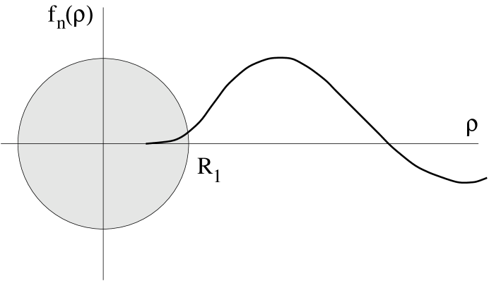
FIG. 1.: A sketch of the mode function $f_{n}$ corresponding to a low-frequency mode of the electromagnetic field, in the presence of a round superconducting wire (of radius $R_{1}$). The sketch is meant to reflect two features: the main support of $f_{n}$ is outside the superconductor, and the value of $f_{n}$ on the surface is much smaller than its typical value outside.

REFERENCES

- [1] S. Khlebnikov, quant-ph/9909024.
- [2] A. O. Caldeira and A. J. Leggett, Ann. Phys. (N.Y.) 149, 374 (1983).
- [3] S. Chakravarty and A. J. Leggett, Phys. Rev. Lett. 52, 5 (1984).
- [4] W. G. Unruh, Phys. Rev. A 51, 992 (1995).
- [5] R. G. Hulet and D. Kleppner, Phys. Rev. Lett. 51, 1430 (1983).
- [6] P. Domokos et al., Phys. Rev. A 52, 3554 (1995); X. Maître et al., Phys. Rev. Lett. 79, 769 (1997).
- [7] L. D. Landau and E. M. Lifshitz, Quantum Mechanics. Nonrelativistic Theory, 3rd ed. (Moscow, Nauka, 1974), Sect. 132 [in Russian].