Laser Cooling of Trapped Fermi Gases deeply below the Fermi Temperature

Abstract

We study the collective Raman cooling of a polarized trapped Fermi gas in the Festina Lente regime, when the heating effects associated with photon reabsorptions are suppressed. We predict that by adjusting the spontaneous Raman emission rates and using appropriately designed anharmonic traps, temperatures of the order of $2.7\%$ of the Fermi temperature can be achieved in 3D.

The realization of atomic Bose-Einstein condensation (BEC) [1] and degenerated Fermi gases [2, 3, 4], are among the most remarkable recent achievements of the Atomic and Condensed-Matter Physics. In the context of these experiments it has been recently proposed [5] that a well-known effect in superconductivity (see e.g. [6]), the BCS transition, could be observable in atomic Fermi gases. The experimental observation of such effect remains, however, as an open challenge. The BCS transition requires temperatures well below the Fermi temperature ($T_{F}$) and, unfortunately, present techniques, based on evaporative cooling in a Fermi gas with two constituents, have not yet been able to reach the required low temperatures. This is due to the Pauli blocking of the atom-atom collisions, which prolongs the cooling into time scales at which technical losses become dominant [7]. Alternative cooling mechanisms [8, 9] combined with the external modification of the scattering length [10], have been proposed as possible mechanisms to achieve BCS.

The aim of this Letter is to show that laser cooling offers a realistic and effective method to cool fermionic samples well below $T_{F}$. Evaporative cooling [2] involves the loss of a large fraction of the initial atoms, which in addition lowers $T_{F}$. On the contrary, laser cooling introduces in principle no atom losses, and therefore allows to cool larger fermionic samples, without significantly lowering $T_{F}$ during the process. In addition, laser cooling allows to cool polarized single–component Fermi gases, in which the atom–atom collisions are almost absent. Once such a polarized gas was sufficiently cooled, an interaction (for instance dipole-dipole one [11]) could be externally induced, which can also lead to BCS transition [12].

Laser cooling of trapped bosons towards BEC have been predicted to work in the Festina Lente (FL) regime [13, 14], in which the spontaneous emission $\gamma$ is smaller than the trap frequency $\omega$. Experimental confirmation of this possibility has been recently reported in Ref. [15]. For fermions, apart from standard problems (reabsorptions), laser cooling is obstacled by the inhibition of spontaneous emission [16]. Such inhibition, combined with the already slow spontaneous emission rate in the FL regime, would lead to unacceptably long cooling times. This Letter shows that both, reabsorption problem and inhibition of the spontaneous emission, can be overcome in the Raman cooling of trapped Fermi gases. This is done first by adjusting the spontaneous Raman rate, and second by employing the anharmonicity of the trap.

We consider $N$ fermions with an accessible electronic three–level $\Lambda$ scheme, with levels $|g\rangle$, $|e\rangle$ and $|r\rangle$. We assume that the ground state $|g\rangle$ is coupled via a Raman transition to $|e\rangle$ (which is assumed metastable). Another laser couples $|e\rangle$ to the upper state $|r\rangle$, which rapidly decays into $|g\rangle$. After the adiabatic elimination of $|r\rangle$, a two–level system is obtained, with an effective Rabi frequency $\Omega$, and an effective spontaneous emission rate $\gamma$. The latter can be controlled by modifying the coupling from $|e\rangle$ to $|r\rangle$. The atoms are confined in a non-isotropic dipole trap with frequencies $\omega^{g}_{x,y,z}$, $\omega^{e}_{x,y,z}$, different for the $|g\rangle$ and $|e\rangle$ states, and non-commensurable one with another. The latter assumption simplifies enormously the dynamics of the spontaneous emission processes in the FL limit. The cooling process consists of sequences of Raman pulses of appropriate frequencies, similar to those of Refs. [14]. We assume weak excitation, so that no significant population in $|e\rangle$ is present. This allows to adiabatically eliminate $|e\rangle$, and consequently to consider only the density matrix $\rho(t)$ describing all atoms in $|g\rangle$, and being diagonal in the Fock representation corresponding to the bare trap levels.

In principle, an inherent heating is introduced by the reabsorption of the spontaneously scattered photons. Fortunately, it has been shown that such heating is largely reduced in the FL regime [13]. Due to the Pauli blocking of the $s$-wave scattering, the elastic collisions can be considered as absent, as well as the collisional two-body and three-body losses. Therefore, the main sources of losses are background collisions and photoassociation. For the considered laser intensities and atomic densities both loss mechanisms are negligible [17], in comparison to the losses introduced by the removal of excited–state atoms discussed below.

In this Letter we use the notation of Refs. [14]. Using the standard theory of quantum stochastic processes one can derive the quantum master equation which describes the atom dynamics in the FL regime. One can then adiabatically eliminate the excited state, to obtain the rate equations for the populations $N_{j}$ in each level of the ground–state trap:

$$\dot{N}_{n}=\sum_{m}\Gamma_{n\leftarrow m}N_{m}-\sum_{m}\Gamma_{m\leftarrow n}N_{n},$$ (1)

where the rates are of the form:

$$\Gamma_{n\leftarrow m} = \frac{\Omega^{2}}{2\gamma}\int_{0}^{2\pi}d\phi\int_{0}^{\pi}d\theta{\cal W}(\theta,\phi)(1-N_{n})$$ (2)

$$\times \left|\sum_{l}\frac{\gamma\eta_{ln}^{\ast}(\vec{k})\eta_{lm}(k_{L})}{[\delta-(\omega_{l}^{e}-\omega_{m}^{g})]+i\gamma(R_{ml}+\Delta_{ml})}\right|^{2},$$ (3)

with

$$R_{ml} = \int_{0}^{2\pi}d\phi\int_{0}^{\pi}d\theta{\cal W}(\theta,\phi)\sum_{n^{\prime}}|\eta_{ln^{\prime}}(\vec{k})|^{2}(1-N_{n^{\prime}}),$$ (4)

and $\Delta_{ml}=\int d\phi\int d\theta{\cal W}(\theta,\phi)|\eta_{lm}(k_{L})|^{2}$. In the above expressions $2\gamma$ is the single–atom spontaneous emission rate, $\Omega$ is the Rabi frequency associated with the atom transition and the laser field, $\eta_{lm}(k_{L})=\langle e,l|e^{i\vec{k}_{L}\cdot\vec{r}}|g,m\rangle$ are the Franck–Condon factors, ${\cal W}(\theta,\phi)$ is the fluorescence dipole pattern, $\omega_{m}^{g}$ ($\omega_{l}^{e}$) are the energies of the ground (excited) trap level $m$ ($l$), and $\delta$ is the laser detuning from the atomic transition [18]. We consider $\Omega<\gamma$ to ensure the validity of the adiabatic elimination of $|e\rangle$.

Note that the rates (3) are nonlinear, due to their quantum statistical dependence on the number of atoms in each level. In particular, we clearly distinguish two different quantum–statistical contributions: (a) If the relevant levels are occupied, $R_{ml}$ vanishes, and the atoms remain for very long times in the excited state $l$, i.e. the spontaneous emission is inhibited. This affects negatively the cooling process in two ways: first, the cooling times become very long, and second, the excited-ground collisions can occur and lead to heating and losses. In addition, the adiabatic elimination used in the derivation of Eq. (1) ceases to be valid. (b) The fermionic inhibition factor $(1-N_{n})$ appears in the numerator of the rates, introducing also a slowing-down of the cooling process.

The above shortcomings can be overcome in the following way. First, note that $\gamma$ can be controlled at will in Raman cooling [13]. One can increase it gradually during the cooling in order to avoid the inhibition effects, but remaining in the FL regime. Still, even if one uses such approach some small fraction of the atoms will remain in the excited state after the cooling pulse, and has to be removed from the trap in order to avoid non-elastic collisions. The latter aim can be achieved by optically pumping the excited atoms to a third non-trapped level. This introduces a new loss mechanism which has to be taken into account in the simulations.

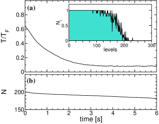
In the following we shall consider a dipole trap characterized by a Lamb-Dicke parameter $\eta=2\pi a/\lambda=2$, with $a=\sqrt{\hbar/2m\omega}$ being the size of the ground state of the trap, and $\lambda$ the laser wavelength. This is the case of current experiments in Mg [19], although our scheme could be also applied to more general traps, and other fermionic species. Let us first consider 1D cooling, as a test of our ideas. Due to numerical demands in the calculation of the Franck-Condon factors for large quantum numbers, we present the results for only $N=200$ fermions, $500$ trap levels, and an initial thermal distribution with $T=0.65T_{F}$, We stress, however, that the method could be employed for larger $N$ and an initial $T>T_{F}$. For Mg atoms and a laser wavelength $\lambda\simeq 600$nm, $\eta=2$ corresponds to a trap frequency $\omega=2\pi\times 5.7$ kHz. A sequence of two pulses with respective detunings $\delta=-15,-16\omega$ was applied. When the system becomes degenerated, the atoms usually jump after a spontaneous emission from $|e\rangle$ into levels of higher energy, since the lower energy levels are occupied. Therefore large negative detunings of the order of four recoil energies are required. Every cooling pulse was assumed to have $\Omega=0.25\omega$ and a duration $t_{p}=100\omega^{-1}$. The spontaneous Raman rate was modified during the cooling process in such a way that the averaged lifetime of the excited atoms was of the order of $0.05t_{p}$. This average was estimated by evaluating the rates (3). The atoms which did not return to $|g\rangle$ after the cooling pulse were removed from the trap.

Fig. 1 (a) shows the time dependence of the temperature, whereas in the inset the final averaged population distribution is depicted. Fig. 1 (b) shows the atomic losses due to removal of the excited atoms with inhibited spontaneous emission. As observed, $T\simeq 0.1T_{F}$ can be reached within $4$ s. In order to achieve such low $T$ with relatively small losses the value of $\gamma$ has been adjusted from an initial value $0.5\omega$ to $8\omega$ in the final stages. Note that this does not imply a departure from the FL regime, since the inhibition effects drastically reduce the effective width of the excited levels. The temperature was calculated from the mean energy $\bar{E}$ with the expression $\bar{E}=0.5NE_{F}(1+(\pi^{2}/3)(T/T_{F})^{2})$, valid for low $T$.

To achieve even a lower $T$, the excitation of atoms deeply placed in the Fermi sea must be avoided. An experimentally feasible method to do it is to use an anharmonic trap, in such a way that the Raman lasers are close to resonance just for the atoms within some desired band of energies; only those atoms are effectively excited. In particular, for strongly degenerated systems one should only excite a band of levels close to the Fermi surface. In the simulations we have used the dependence $\omega_{n}^{e,g}=\omega n(1-\alpha n)$ for the trap levels, where $\alpha$ is the anharmonicity parameter [20]. Sufficiently small anharmonicity does not affect the Franck-Condon factors, but it does influence the resonance term in the denominator of the rates (3). The requirement that the pulse resonant with the transition $\omega_{m+s}^{e}-\omega_{m}^{g}$, affects only the atoms occupying the band of energies around $m$, put on $\alpha$ the following constrain: $\alpha m_{max}<1/4|s|$ with $m_{max}$ the maximum level considered in the simulation. This inequality has to be fulfilled for each cooling pulse. The width $\delta_{m}$ of the affected band is related to $\gamma$. Comparison of the two terms in the denominator of (3) leads to the following formula $\gamma\sim\alpha s\delta_{m}\omega/(4R_{m,m+s})$ [21].

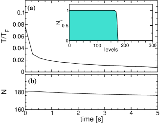
We have considered a fermionic gas, already pre-cooled by the previous method, with an initial $T=0.08T_{F}$ and $N=181$ ($10\%$ of the above considered initial number $200$ is lost during the first stage of cooling). The trap parameters were chosen as above, except for the addition of a small anharmonicity $\alpha=1.04\times 10^{-5}$. Such $\alpha$, and a value $\gamma=0.02\omega$ were chosen to allow for transitions inside a band of about $20$ levels. The cooling scheme consist of two pulses with detunings designed to be resonant with the transition from the Fermi level ($181$) and $47$ and $48$ levels below respectively. Those large detunings are necessary to fill the holes deep inside the Fermi sea by the atoms from the surface. Both pulses have $\Omega=0.016\omega$ and a quite long duration $t_{p}=5000\omega^{-1}$. The latter is necessary due to the slow Raman spontaneous process in a deeply degenerated system. The losses in this case are negligible ($\sim 1\%$) mainly due to the long pulses used.

Fig. 2 (a) shows the time dependence of the temperature, whereas its inset shows the final atom distribution. At the end of this cooling stage (after $5$ s) the temperature decreases down to $0.01T_{F}$. Fig. 2 (b) shows the atomic losses due to the removal of the excited atoms with inhibited spontaneous emission.

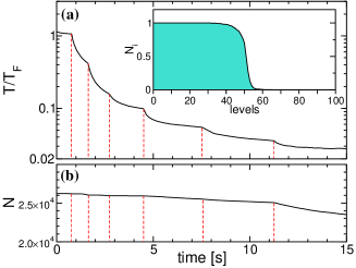
Finally, we have analyzed the more interesting case of a 3D cooling. For simplicity we have considered an isotropic trap, in which the level energies have a dependence similar to the 1D case [22]. We have taken $N=26235$ atoms, $101$ energy shells ($176851$ levels), and an initial thermal distribution with $T=1.14T_{F}$. At $T=0$ the atoms fill $53$ complete energy shells. In this case the method of increasing $\gamma$ during the duration of the pulses was not used, and thus a rather complex sequence of pulses was employed. The cooling was divided into $7$ stages, each one of them consisting in cycles of two Raman pulses with detunings $\delta/\omega=\{$$(-6,-7)$, $(-14,-15)$, $(-19,-20)$, $(-19,-20)$, $(-18,-19)$, $(-20,-18)$, $(-20,-18)\}$, and tuned to induce transitions from the bands centered at the shells $\{16$, $40$, $90$, $70$, $61$, $(53,57)$, $56\}$ with respective widths of $\{20$, $28$, $60$, $40$, $40$, $(40,10)$, $20\}$ levels. The spontaneous emission rates were chosen $\gamma/\omega=\{$$(0.0075,0.0088)$, $(0.025,0.026)$, $(0.071,0.075)$, $(0.048,0.05)$, $(0.045,0.048)$, $(0.48,0.028)$, $(0.15,0.07)\}$. The detunings were chosen taking into account the 3D character of the trap states, since the excitation quantum number can only be decreased in one direction in one cooling cycle. The first four pulses redistribute atoms occupying the levels below $E_{F}$, making this part of the system more degenerate, next six pulses empty the trap levels well above $E_{F}$ and the last four affect the band around $E_{F}$. We use $\Omega=0.8\gamma$ in each pulse, except in the $11$–th where $\Omega=0.1\gamma$, to ensure the validity of the adiabatic elimination.

Fig. 3 shows: (a) the time dependence of $T/T_{F}$ during the cooling (solid line), and (b) the atom losses. The temperature was calculated with the help of the grand canonical expressions for the mean values of the particle number and energy. At the end of the process ($t=13$s) the system reached $T=0.027T_{F}$. In the simulations we assumed that a fraction of the order of $1\%$ of atoms is excited in every pulse, except sixth stage where there was about $7\%$ excited atoms in every pulse. If such fraction is kept constant, similar cooling times are expected for larger $N$, the only limitation being the photoassociation losses.

Our analysis can be extended to the case of a multi–component Fermi gas. In such a case, the different species can interact via $s$-wave scattering, although for a sufficiently degenerated gas such collisions should be largely suppressed, and in practice only possible close to the Fermi surface, inducing a perturbative modification of the trap levels. The collisional dynamics can be split from the laser cooling dynamics [23], and can be studied within the formalism of Quantum-Boltzmann-Master-Equation [23, 24]. The collisions will introduce a thermalization effect, which in fact should help in the cooling. The case of an unpolarized Fermi gas is particularly interesting when the interaction between different species is attractive, since in such a case BCS pairing should be possible for temperatures below a critical value $T_{c}$. For reasonable densities and scattering lengths, $T_{c}$ is well below $T_{F}$, and beyond the reach of the present evaporative cooling techniques. The methods discussed in our Letter offer an interesting perspective in this sense, since they allow to reach $T\ll T_{F}$.

Polarized Fermi gases are by themselves also interesting, since once the gas had acquired a sufficiently low $T$, an interaction, such as for instance dipole-dipole one [11], could be externally induced. Such interaction, partially attractive, allows for the appearance of BCS transition [12]. BCS transition in a dipolar gas presents clear advantages compared to the one generated in a two-species gas, since for the latter the precise matching of both Fermi surfaces is essential, and experimentally very demanding.

Finally, let us point that the full description of the laser-induced BCS transition within the Master Equation formalism remains as a fascinating challenge. Such analysis will be the subject of future investigations.

We acknowledge support of the Deutsche Forschungsgemeinschaft (SFB 407), ESF PESC BEC2000+, and TMR ERBXTCT96-0002. Z. I. was additionally supported by Polish KBN Grant No. 5 P03B 103 20 and the Subsidy of the Foundation for Polish Science. Fruitful discussions with M. Baranov, T. Mehlstäubler, J. Keupp, E. Rasel, and K. Sengstock are acknowledged.

FIG. 1.: 1D cooling by using the controlled Raman rate: (a) time dependence of the temperature and (b) losses. Inset: final averaged distribution. For details, see text.

FIG. 2.: 1D cooling by using the anharmonicity of the trap: (a) time dependence of the temperature and (b) losses. Inset: final averaged distribution. For details, see text.

FIG. 3.: 3D cooling by using the anharmonicity of the trap: (a) time dependence of the temperature and (b) losses. Dashed lines separate different stages of the cooling process. Inset: final averaged distribution. For details, see text.

REFERENCES

- [1] M. H. Anderson et al., Science 269, 198 (1995); K.B. Davis et al., Phys. Rev. Lett. 75, 3969 (1995); C. C. Bradley et al., ibid 75, 1687 (1995); 79, 1170 (1997).
- [2] B. DeMarco and D. S. Jin, Science 285, 1703 (1999).
- [3] F. Schreck et al., Phys. Rev. A 64, 011402R (2001); F. Schreck et al, Phys. Rev. Lett. 87, 080403 (2001).
- [4] A. G. Truscott et al., Science 291, 2570 (2001).
- [5] H.T.C. Stoof et al., Phys. Rev. Lett. 76, 10 (1996); M. A. Baranov et al., JETP Lett. 64, 301 (1996); M. Houbiers et al., Phys. Rev. A 56, 4864 (1997).
- [6] P. G. de Gennes, Superconductivity in metals and alloys (W. A. Benjamin, New York, 1966)
- [7] M. J. Holland et al., Phys. Rev. A 61, 053610 (2000)
- [8] L. Viverit et al., cond-mat/0005517.
- [9] G. Ferrari and C. Salomon, private communication.
- [10] J. Stenger et al., Phys. Rev. Lett. 82, 2422 (1999); S. L. Cornish et al., ibid 85, 1795 (2000).
- [11] S. Yi, and L. You, Phys. Rev. A 61, 041604 (2000); K. Góral et al., ibid 61, 051601 (2000); L. Santos et al., Phys. Rev. Lett. 85, 1791 (2000).
- [12] L. You and M. Marinescu, Phys. Rev. A 60, 2324 (1999); M. A. Baranov et al., in preparation.
- [13] Y. Castin et al., Phys. Rev. Lett. 80, 5305 (1998).
- [14] L. Santos and M. Lewenstein, Eur. Phys. J. D 7, 379 (1999); L. Santos and M. Lewenstein, Phys. Rev. A 60, 3851 (1999).
- [15] S. Wolf, S. J. Oliver, and D. S. Weiss, Phys. Rev. Lett. 85, 4249 (2000).
- [16] T. Busch et al., Europhys. Lett. 44, 1 (1998); B. DeMarco and D.S. Jin, Phys. Rev. A 58, R4267 (1998); J. Ruostekoski and J. Javanainen, Phys. Rev. Lett. 82, 4741 (1999).
- [17] Background collisions depend on the technical limitations, and for rates of the order of Hz [7] can be safely ignored in our simulations. Photoassociation losses (when the laser is tuned between molecular resonances) are typically of the order of cm3/s for laser intensities of mW/cm2 (see e.g. M. Machholm et al, Phys. Rev. A 59, R4113 (1999)). In our case the laser intensities needed are typically times smaller, and therefore photoassociation losses can be neglected, since we keep the densities smaller than cm-3.
- [18] Conservative dipole–dipole interactions do not play a significant role at the considered densities (cm3), and are omitted. Their role is discussed in Refs. [14, 23].
- [19] Laser cooling of Mg is currently experimentally studied by E. Rasel and W. Ertmer (private communication).
- [20] For instance, by superimposing a red detuned Gaussian laser beam, or a magnetic trap, with a blue-detuned higher Laguerre-Gauss beam, one can design a combination of harmonic and quartic potential; for experiments see K. Bongs et al., Phys. Rev. A 63, 031602 (2001).
- [21] The coefficient depends on the atom distribution, therefore in the calculation of the effect of increasing degeneracy has to be taken into account.
- [22] Anharmonic trap may be designed in such a way that the energy levels , depend only on , i.e. the energy of unperturbed trap. Such dependence requires the presence of cross terms (like ) in the perturbative potential. Eventually, a potential in which the , and dependences are separated could also be used, although such potential may lead to some accidental degeneracies for transitions well below the Fermi level.
- [23] L. Santos and M. Lewenstein, Appl. Phys. B 69, 363 (1999).
- [24] C. Gardiner and P. Zoller, Phys. Rev. A 55, 2902 (1997); D. Jaksch et al., ibid 56, 575 (1997).