Vacuum Induced Coherences in Radiatively Coupled Multilevel Systems

Abstract

We show that radiative coupling between two multilevel atoms having near-degenerate states can produce new interference effects in spontaneous emission. We explicitly demonstrate this possibility by considering two identical V systems each having a pair of transition dipole matrix elements which are orthogonal to each other. We discuss in detail the origin of the new interference terms and their consequences. Such terms lead to the evolution of certain coherences and excitations which would not occur otherwise. The special choice of the orientation of the transition dipole matrix elements enables us to illustrate the significance of vacuum induced coherence in multi-atom multilevel systems. These coherences can be significant in energy transfer studies.

PACS No. : 42.50.Fx, 42.50.Ct, 42.50.Md

I Introduction

A multilevel atom having closely lying energy states (energy separation of the order of the natural linewidth) can show interferences in the decays from those closely lying levels to a common ground state. This is due to the fact that, both the decay channels are coupled via the same continuum of the vacuum, creating the interfering path ways. The resulting coherence in the system is known as vacuum induced coherence (VIC). Occurrence of this coherence requires a stringent but achievable condition - i.e. the transition dipole matrix elements involving the decay processes should be non-orthogonal [1]. The manifestation of VIC in atomic systems has given rise to a myriad of fascinating phenomena [1-17]. All these studies deal with a single multilevel atom or equivalently with an ensemble of non-interacting multilevel atoms (e.g. very low density atomic gas systems). However, VIC in coupled atomic systems has remained unexplored. In this paper, we consider the role of VIC in two radiatively coupled multilevel atoms.

We start by recalling some of the consequences of VIC in a single atom. It was first shown by Agarwal [1] that population gets trapped in degenerate excited states of an atom due to interference in decays channels. Recently, there has been renewed interest in this subject particularly in the context of coherently driven systems [2, 3, 4, 5]. Harris and Imamoğlu were the first to discover the possibility of achieving lasing without population inversion in systems where two excited states were coupled to a common continuum [6] (See also [7, 8]). It has also been been observed that narrowing of spontaneous emission can be obtained by making use of the VIC [3, 9]. Quantum beat has been observed in spontaneous emission which showed pronounced beat structures determined by the energy separation of the closely lying states [10, 11]. The VIC also leads to cancellation of spontaneous emission [12, 13, 14]. Zhu and coworkers have experimentally demonstrated the quenching of spontaneous emission in sodium dimers [12]. Further Scully, Zhu and coworkers proposed many schemes with different configurations demonstrating the possibility of obtaining quenching of spontaneous emission [13]. It was also reported that in the presence of VIC, the resonance fluorescence [15, 16] and other spectral line shapes [5] become sensitive to the phase of the control laser. Knight and coworkers [16] have demonstrated the possibility of controlling spontaneous emission by varying the relative phase of two control lasers in a four-level system. The question of requirement of non-orthogonal dipole moments has been addressed and alternative possibilities have been suggested [11, 12, 14, 17].

All the above works [2-17] correspond to a single atom system, or equivalently an ensemble of non-interacting atoms where the average inter-atomic distance is much larger compared to the wavelength of the emitted radiation. However, when the inter-atomic distance becomes comparable to the wavelength, the dipole-dipole (dd) coupling between the atoms via vacuum gives rise to collective effects. Our usage of dd interaction should be understood in the sense of retarded (and complex) dipole-dipole interaction. The classic example is Dicke superradiance [18], where the atoms in their excited state decay much faster compared to that of the single atom case. The collective effects in atoms have been extensively studied [18-30]. Recently experiments have been reported to observe collective behavior with two identical atoms [19, 20]. The dd interaction has been shown to produce two-photon resonance [21] and frequency shifts in emission [22]. The energy exchange between two coupled systems is discussed in [23]. Many interesting features of dd interaction in the context of atoms interacting with a squeezed vacuum [24], and inside bandgap materials [25] have been reported. Mayer and Yeoman [26] have considered two-atom laser in the presence of the atom-atom interaction. Quantum jump from two dipole interacting V-systems giving rise to new fluorescence periods has been reported by Hegerfeldt and coworkers [27]. Meystre and coworkers [28] found that the dd interaction leads to the occurrence of dark states in the fluorescence of two moving atoms [29]. Finally note that the local field effects in a dense media are also a consequence of dd interaction [30]. All the dd interaction related effects can be understood as due to the exchange of virtual photons between the atoms. Most of the existing literature concerns two-level atoms.

In this paper, we consider two identical V-systems having two closely lying excited states (as shown in Fig. 1). The two atoms get coupled by the exchange of radiation. We would specifically show how the radiative coupling in multilevel systems can lead to a population transfer from $|1_{A}\rangle$ to $|2_{B}\rangle$ even if the corresponding dipole matrix elements are orthogonal.

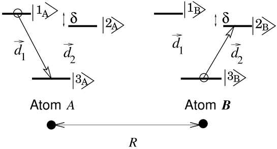
FIG. 1.: The two identical $V$ systems under consideration. The distance between the two atoms is $R$. The transition dipole matrix elements $\vec{d}_{1}$ and $\vec{d}_{2}$ are chosen to be orthogonal with each other. The energy separation between the excited states is $\hbar\delta$. We discuss the situation where initially atom $A$ is in excited state $|1_{A}\rangle$ and atom $B$ is in ground state $|3_{B}\rangle$. Possibility of dd interaction induced excitation in the $|3_{B}\rangle\rightarrow|2_{B}\rangle$ transition is indicated.

The organization of the paper is the following: In Sec. II we derive the equations for the dynamical evolution of the two V-systems in master equation formalism. In Sec. III we interpret the terms appearing in the master equation and discuss the dependence of these terms on the geometry of the atoms in detail. In Sec.IV we present the numerical results on the evolution of the excited state coherence and the excitation probabilities. In Sec. V we present results for the case of magnetic degeneracies and we also discuss how the new coherence effect can be monitored. In Sec.VI we present the concluding remarks.

II Dynamical Evolution of Two V-systems

We consider [Fig. 1] two identical V-systems (say A and B) in free space, having two near-degenerate excited states $|1_{\mu}\rangle$ and $|2_{\mu}\rangle$ ($\mu=A,B$) with the level separation $\hbar\delta$. The ground states of the atoms are represented by $|3_{\mu}\rangle$. Let $\omega_{1}$ and $\omega_{2}$ be the atomic frequencies corresponding to $|1_{\mu}\rangle\leftrightarrow|3_{\mu}\rangle$ and $|2_{\mu}\rangle\leftrightarrow|3_{\mu}\rangle$ transitions respectively. Let the position vectors of the atoms be $\vec{x}_{A}$ and $\vec{x}_{B}$. Both the atoms couple with the vacuum field, which is given by

$$\vec{E}_{v}(\vec{x})=\vec{E}^{(+)}(\vec{x})+\vec{E}^{(-)}(\vec{x});$$ (1)

where $\vec{E}^{(+)}~{}(\vec{E}^{(-)})$ represents the positive (negative) frequency part the vacuum field at $\vec{x}$ and is defined as

$$\vec{E}^{(+)}(\vec{x})=\sum_{k,s}i\left(\frac{2\pi\hbar\omega_{k}}{V}\right)^{1/2}\hat{a}_{ks}\hat{\epsilon}_{ks}e^{i\vec{k}\cdot\vec{x}},$$ (2)

and $\vec{E}^{(-)}$ is the Hermitian conjugate of $\vec{E}^{(+)}$. Here $\hat{a}_{ks}~{}(\hat{a}_{ks}^{{\dagger}})$ represent the annihilation (creation) operator of a field mode having propagation vector $\vec{k}$ and polarization $s$; $\omega_{k}(=kc)$ represents the angular frequency corresponding to the $k$-mode. The corresponding unit polarization vector is denoted by $\hat{\epsilon}_{ks}$.

In what follows we consider the following physical process: Initially atom $A$ is taken to be in excited state $|1_{A}\rangle$ and the second atom in ground state $|3_{B}\rangle$. To highlight the effect of new interference terms, we specifically consider the case when the two transition dipole matrix elements $\vec{d}_{1}$ and $\vec{d}_{2}$ are orthogonal to each other. In the absence of atom $B$, the VIC cannot be created in the excited states of atom $A$ because the transition dipole matrix elements $\vec{d}_{1}$ and $\vec{d}_{2}$ are orthogonal. However, the radiative coupling can lead to evolution of the excited state coherences. We will also show a manifestation of this coherence in the dynamical evolution of the atomic population.

The total Hamiltonian for the atoms and the field system is given by

$$H=H_{a}+H_{f}+H_{I},$$ (3)

where the unperturbed Hamiltonian for the atoms and field are

$$H_{a}=\hbar\sum_{\mu=A,B}\left(\omega_{1}\hat{\alpha}_{\mu}^{\dagger}\hat{\alpha}_{\mu}+\omega_{2}\hat{\beta}_{\mu}^{\dagger}\hat{\beta}_{\mu}\right),$$ (4)

$$H_{f}=\sum_{ks}\hbar\omega_{ks}\hat{a}_{ks}^{\dagger}\hat{a}_{ks},$$ (5)

and the interaction Hamiltonian is

$$H_{I} = -\vec{d}.\vec{E}_{v}$$ (6)

$$= -\sum_{j=1}^{2}\left[\vec{d}_{j3}^{~{}(\mu)}\cdot\vec{E}_{v}(\vec{x}_{\mu})+h.c.\right]~{}~{}(\mu=A,~{}B).$$ (7)

The atomic transition operators introduced in (4), are given by

$$\hat{\alpha}_{\mu}\equiv|3_{\mu}\rangle\langle 1_{\mu}|,~{}~{}\hat{\beta}_{\mu}\equiv|3_{\mu}\rangle\langle 2_{\mu}|,$$ (8)

$$\hat{\alpha}_{\mu}^{{\dagger}}\equiv|1_{\mu}\rangle\langle 3_{\mu}|,~{}~{}\hat{\beta}_{\mu}^{{\dagger}}\equiv|2_{\mu}\rangle\langle 3_{\mu}|.$$ (9)

Thus $\hat{\alpha}_{\mu},\hat{\alpha}_{\mu}^{{\dagger}}$ ($\hat{\beta}_{\mu},\hat{\beta}_{\mu}^{{\dagger}}$) represent the atomic lowering and raising operators respectively corresponding to the $|1_{\mu}\rangle\leftrightarrow|3_{\mu}\rangle$ ($|2_{\mu}\rangle\leftrightarrow|3_{\mu}\rangle$) transition. The dipole matrix elements are represented by

$$\vec{d}_{j3}^{~{}(\mu)}=\vec{d}_{j}^{~{}(\mu)}|j_{\mu}\rangle\langle 3_{\mu}|.$$ (10)

For simplicity we consider a situation where the transition dipole matrix elements of atom $A$ are parallel to the transition dipole matrix elements of atom $B$

$$\vec{d}_{13}^{~{}(A)}~{}||~{}\vec{d}_{13}^{~{}(B)}~{}~{}{\rm and}~{}~{}\vec{d}_{23}^{~{}(A)}~{}||~{}\vec{d}_{23}^{~{}(B)}.$$ (11)

We also assume that

$$\vec{d}_{13}^{~{}(A)}\cdot\vec{d}_{23}^{~{}(A)^{*}}=0.$$ (12)

Thus the index $\mu$ in the right hand side of Eq. (10) can be dropped and the dipole matrix elements can be rewritten as

$$\vec{d}_{j3}^{~{}(\mu)}=\vec{d}_{j}|j_{\mu}\rangle\langle 3_{\mu}|.$$ (13)

Here we note that $\vec{d}_{j}$, in general, can be complex (see for example Sec.V). Using Eq. (13), the interaction Hamiltonian in (6) reduces to

$$H_{I}=-\sum_{\mu=A,B}\left[\left(\vec{d}_{1}\hat{\alpha}_{\mu}^{\dagger}+\vec{d}_{2}\hat{\beta}_{\mu}^{\dagger}\right)\cdot\vec{E}_{v}(\vec{x}_{\mu})+h.c.\right].$$ (14)

We work in the interaction picture by transforming (14)

$$H_{I}(t) = e^{\frac{i}{\hbar}(H_{a}+H_{f})t}H_{I}e^{-\frac{i}{\hbar}(H_{a}+H_{f})t}$$ (15)

$$= -\sum_{\mu=A,B}\left[\left(\vec{d}_{1}\hat{\alpha}_{\mu}^{\dagger}e^{i\omega_{1}t}+\vec{d}_{2}\hat{\beta}_{\mu}^{\dagger}e^{i\omega_{2}t}\right)\cdot\left(\vec{E}^{(+)}(\vec{x}_{\mu},t)+\vec{E}^{(-)}(\vec{x}_{\mu},t)\right)+h.c.\right];$$ (16)

where,

$$\vec{E}^{(+)}(\vec{x}_{\mu},t)=\sum_{k,s}i\left(\frac{2\pi\hbar\omega_{k}}{V}\right)^{1/2}\hat{a}_{ks}\hat{\epsilon}_{ks}e^{i(\vec{k}\cdot\vec{x}_{\mu}-\omega_{k}t)}~{}~{}{\rm and}~{}~{}\vec{E}^{(-)}(\vec{x}_{\mu},t)=[\vec{E}^{(+)}(\vec{x}_{\mu},t)]^{{\dagger}}.$$ (17)

Let the density operator of the combined atom-field system in the interaction picture be represented by $\rho(t)$ which satisfies the Liouville equation of motion

$$\frac{\partial\rho}{\partial t}=-\frac{i}{\hbar}\left[H_{I}(t),\rho\right].$$ (18)

To derive useful information about the evolution of the atomic system, we derive a master equation for the reduced atomic operator by using the standard projection operator techniques [1]. We make certain approximations in deriving the master equation: (a) at $t=0$, $\rho(0)$ can be factorized into a product of atom [$\rho_{a}$] and field [$\rho_{f}$] density operators, i.e. $\rho(0)\equiv\rho_{a}(0)\rho_{f}(0)$. Furthermore, we invoke (b) the Born approximation and (c) the Markoff approximation. The Born approximation depends on the weak coupling between the vacuum and the atoms. The Markoff approximation holds because the vacuum has fairly flat density of states. Using the above approximations and tracing over the field states, the density matrix equation for the atoms becomes

$$\frac{\partial{\rho_{a}}}{\partial t}=-\frac{1}{\hbar^{2}}\lim_{t\rightarrow\infty}\int_{0}^{t}d\tau{\rm Tr}_{f}\left[H_{I}(t),[H_{I}(t-\tau),\rho_{f}(0){\rho_{a}}]\right].$$ (19)

The trace over the field operators inside the integral in Eq. (19) is calculated using the following relations:

$${\rm Tr}_{f}(\rho_{f}a^{\dagger}_{ks}a_{k^{\prime}s^{\prime}})=0,~{}{\rm Tr}_{f}(\rho_{f}a_{ks}a^{\dagger}_{k^{\prime}s^{\prime}})=\delta_{kk^{\prime}}\delta_{ss^{\prime}},$$ (20)

$${\rm Tr}_{f}(\rho_{f}a_{ks}a_{k^{\prime}s^{\prime}})={\rm Tr}_{f}(\rho_{f}a^{\dagger}_{ks}a^{\dagger}_{k^{\prime}s^{\prime}})=0.$$ (21)

One also uses the rotating wave approximation (RWA) to drop the anti-resonant terms like $\hat{\alpha}_{\mu}\hat{\alpha}_{\mu}$, $\hat{\alpha}_{\mu}^{\dagger}\hat{\alpha}_{\mu}^{\dagger}$, $\hat{\beta}_{\mu}\hat{\beta}_{\mu}$ and $\hat{\beta}_{\mu}^{\dagger}\hat{\beta}_{\mu}^{\dagger}$ in (19). Using the above conditions and carrying out a long algebra, we obtain the master equation for the atomic density operator

$$\frac{\partial\rho}{\partial t}= - \left[\left\{\gamma_{1}\sum_{\mu=A,B}\left(\hat{\alpha}_{\mu}^{\dagger}\hat{\alpha}_{\mu}\rho-2\hat{\alpha}_{\mu}\rho\hat{\alpha}_{\mu}^{\dagger}+\rho\hat{\alpha}_{\mu}^{\dagger}\hat{\alpha}_{\mu}\right)\right\}+1\rightarrow 2,~{}\alpha\rightarrow\beta\right]$$ (22)

$$- \left[\Gamma_{1}\left\{(\hat{\alpha}_{A}^{\dagger}\hat{\alpha}_{B}\rho-2\hat{\alpha}_{B}\rho\hat{\alpha}_{A}^{\dagger}+\rho\hat{\alpha}_{A}^{\dagger}\hat{\alpha}_{B})+~{}{\rm h.c.}\right\}+1\rightarrow 2,~{}\alpha\rightarrow\beta\right]$$ (23)

$$+ \left[\left\{i\Omega_{1}[\hat{\alpha}_{A}^{\dagger}\hat{\alpha}_{B},\rho]+h.c.\right\}+1\rightarrow 2,~{}\alpha\rightarrow\beta\right]$$ (24)

$$- \left[\left\{\Gamma_{vc}\left(\hat{\beta}_{A}^{\dagger}\hat{\alpha}_{B}\rho-2\hat{\alpha}_{B}\rho\hat{\beta}_{A}^{\dagger}+\rho\hat{\beta}_{A}^{\dagger}\hat{\alpha}_{B}\right)e^{-i\delta t}+h.c.\right\}+A\leftrightarrow B\right]$$ (25)

$$+ \left[\left\{i\Omega_{vc}[\hat{\beta}_{A}^{\dagger}\hat{\alpha}_{B},\rho]e^{-i\delta t}+h.c.\right\}+A\leftrightarrow B\right];$$ (26)

where,

$$\gamma_{i} = \sum_{k,s}\left(\frac{2\pi\omega_{k}}{\hbar V}\right)\pi\delta(\omega_{0}-\omega_{k})|\vec{d}_{i}\cdot\hat{\epsilon}_{ks}|^{2},$$ (27)

$$\Gamma_{i} = \sum_{k,s}\left(\frac{2\pi\omega_{k}}{\hbar V}\right)\pi\delta(\omega_{0}-\omega_{k})|\vec{d}_{i}\cdot\hat{\epsilon}_{ks}|^{2}e^{i\vec{k}\cdot\vec{R}},$$ (28)

$$\Omega_{i} = \sum_{k,s}\left(\frac{2\pi\omega_{k}}{\hbar V}\right)\left(\frac{1}{\omega_{0}-\omega_{k}}-\frac{1}{\omega_{0}+\omega_{k}}\right)|\vec{d}_{i}\cdot\hat{\epsilon}_{ks}|^{2}e^{i\vec{k}\cdot\vec{R}},$$ (29)

$$\Gamma_{vc} = \sum_{k,s}\left(\frac{2\pi\omega_{k}}{\hbar V}\right)\pi\delta(\omega_{0}-\omega_{k})(\vec{d}_{2}\cdot\hat{\epsilon}_{ks})(\vec{d}_{1}\cdot\hat{\epsilon}_{ks})^{*}e^{i\vec{k}\cdot\vec{R}},$$ (30)

$$\Omega_{vc} = \sum_{k,s}\left(\frac{2\pi\omega_{k}}{\hbar V}\right)\left(\frac{1}{\omega_{0}-\omega_{k}}-\frac{1}{\omega_{0}+\omega_{k}}\right)(\vec{d}_{2}\cdot\hat{\epsilon}_{ks})(\vec{d}_{1}\cdot\hat{\epsilon}_{ks})^{*}e^{i\vec{k}\cdot\vec{R}}.$$ (31)

Here, $\vec{R}=\vec{x}_{A}-\vec{x}_{B}$. Since the states $|1_{\mu}\rangle$ and $|2_{\mu}\rangle$ are closely lying, we have set $\omega_{1}\cong\omega_{2}\equiv\omega_{0}$. The suffix $a$ of $\rho_{a}$ in Eq. (26) has been dropped for brevity. We have also dropped the Lamb shift terms associated with the spontaneous emission of the individual atoms. The summation over the polarization components is evaluated using the relation

$$\sum_{s}(\hat{\epsilon}_{ks})_{\mu}(\hat{\epsilon}_{ks}^{*})_{\nu}\equiv\delta_{\mu\nu}-\hat{k}_{\mu}\hat{k}_{\nu},$$ (32)

where $\hat{k}_{l}$ represents the direction cosine of $\vec{k}/|\vec{k}|$ along the $l^{th}$ Cartesian axis. Taking the limit $V\rightarrow\infty$ and replacing the summation over $k$ by integration over the continuum of the field modes, the terms in (27) become

$$\gamma_{i}=\frac{2|\vec{d}_{i}|^{2}}{3\hbar}\left(\frac{\omega_{0}}{c}\right)^{3}$$ , (33)

$$\Gamma_{i}=\frac{1}{\hbar}~{}(\vec{d}_{i}\cdot{\rm Im}~{}\stackrel{{\scriptstyle\Rightarrow}}{{\chi}}\cdot\vec{d}_{i}^{*}) ~{}~{}\Omega_{i}=\frac{1}{\hbar}~{}(\vec{d}_{i}\cdot{\rm Re}~{}\stackrel{{\scriptstyle\Rightarrow}}{{\chi}}\cdot\vec{d}_{i}^{*}),$$ , (34)

$$\Gamma_{vc}=\frac{1}{\hbar}~{}(\vec{d}_{2}\cdot{\rm Im}~{}\stackrel{{\scriptstyle\Rightarrow}}{{\chi}}\cdot\vec{d}_{1}^{*}) ~{}~{}\Omega_{vc}=\frac{1}{\hbar}~{}(\vec{d}_{2}\cdot{\rm Re}~{}\stackrel{{\scriptstyle\Rightarrow}}{{\chi}}\cdot\vec{d}_{1}^{*});$$ , (35)

where $\stackrel{{\scriptstyle\Rightarrow}}{{\chi}}$ is a tensor whose components are given by

$$\chi_{\mu\nu}(\vec{x}_{A},\vec{x}_{B},\omega_{0}) \equiv \left(k_{0}^{2}\delta_{\mu\nu}+\frac{\partial^{2}}{\partial{x_{A}}_{\mu}\partial{x_{A}}_{\nu}}\right)\frac{e^{ik_{0}R}}{R}~{}~{}~{}~{}~{}(k_{0}=\omega_{0}/c)$$ (36)

$$\equiv \left[\delta_{\mu\nu}\left(\frac{k_{0}^{2}}{R}+\frac{ik_{0}}{R^{2}}-\frac{1}{R^{3}}\right)-R_{\mu}R_{\nu}\left(\frac{k_{0}^{2}}{R^{3}}+\frac{3ik_{0}}{R^{4}}-\frac{3}{R^{5}}\right)\right]e^{ik_{0}R};R=|\vec{x}_{A}-\vec{x}_{B}|.$$ (37)

III Interpretation of different terms in the master equation (18)

The $2\gamma_{i}$ in Eq. (33) represents the single atom spontaneous decay rate from the state $|i\rangle$ to the state $|3\rangle$. Rest of the coefficients in (26) are related to the coupling between the two $V$-systems. This coupling is produced by the exchange of a photon between the two systems. The dipole-dipole interaction manifests itself through the tensor $\stackrel{{\scriptstyle\Rightarrow}}{{\chi}}$ defined by Eq. (36). The tensor $\stackrel{{\scriptstyle\Rightarrow}}{{\chi}}_{\alpha\beta}(\vec{x}_{A},\vec{x}_{B},\omega)$ has the following meaning: It represents the $\alpha^{th}$ component of the electric field at the point $\vec{x}_{A}$, produced by an oscillating dipole of unit strength along the direction $\beta$ and located at the point $\vec{x}_{B}$ [31]. In the limit $c\rightarrow\infty$ ($k_{0}\rightarrow 0$), it reduces to the static dipole-dipole interaction. $\Gamma_{i}$ and $\Omega_{i}$ represent the dd couplings which are related to the decay and level shift of the collective atomic states. These coefficients couple a pair of parallel dipoles and are well known [1], particularly in the context of collective effects in two level atoms. The new coherence terms $\Gamma_{vc}$ and $\Omega_{vc}$ are the dipole-dipole cross coupling coefficients, which couple a pair of orthogonal dipoles. The meaning of such terms can be clearly understood by calculating the evolution of the population in the state $|3_{A},2_{B}\rangle$, given the initial condition $|1_{A},3_{B}\rangle$. From the master equation (26), one can show that at $t\approx 0$,

$$\frac{\partial}{\partial t}\langle 1_{A},3_{B}|\rho|3_{A},2_{B}\rangle=-(\Gamma_{vc}^{*}+i\Omega_{vc}^{*})e^{i\delta t},$$ (38)

and hence

$$\frac{\partial}{\partial t}\langle 3_{A},2_{B}|\rho|3_{A},2_{B}\rangle = -(\Gamma_{vc}-i\Omega_{vc})e^{-i\delta t}\langle 1_{A},3_{B}|\rho|3_{A},2_{B}\rangle$$ (40)

$$-(\Gamma_{vc}^{*}+i\Omega_{vc}^{*})e^{i\delta t}\langle 3_{A},2_{B}|\rho|1_{A},3_{B}\rangle$$

$$= -2|\Gamma_{vc}-i\Omega_{vc}|^{2}\left(\frac{\sin\delta t}{\delta}\right).$$ (41)

Thus to the lowest order in $\Gamma_{vc}$ and $\Omega_{vc}$, we obtain

$$\langle 3_{A},2_{B}|\rho|3_{A},2_{B}\rangle\approx 4|\Gamma_{vc}+i\Omega_{vc}|^{2}\left(\frac{\sin^{2}(\delta t/2)}{\delta^{2}}\right).$$ (42)

Therefore the radiative process, in which atom $A$ in the excited state $|1_{A}\rangle$ loses its excitation which in turn excites atom $B$ to the state $|2_{B}\rangle$, is possible only because of $\Gamma_{vc}$ and $\Omega_{vc}$ terms in the master equation (26). Note further that such terms start becoming insignificant as $\hbar\delta$ - the energy separation between the two excited states increases. Such interference terms occur in the master equation even when the transition dipole matrix elements $\vec{d}_{1}$ and $\vec{d}_{2}$ are orthogonal. Such contributions come from the second term in Eq. (36). In the rest of the paper, we study in detail various consequences of these interference terms which could be large and could significantly contribute to the dynamics of the system when the atomic separation is smaller than $\lambda$.

Let us consider a geometry where atom $A$ is placed at the origin of a Cartesian co-ordinate system and the position vector of atom $B$ is $\vec{R}$ (as shown in Fig. 2). $\vec{R}$ makes an angle $\theta$ with the $z$ axis. Let us assume $\vec{d}_{1}=\hat{x}d$ and $\vec{d}_{2}=\hat{y}d$. All the radiative coupling terms in the master equation can be written down explicitly as

$$\Gamma_{1}=\frac{|d|^{2}}{\hbar}{\rm Im}~{}\chi_{xx}=\frac{3\gamma}{2}(P_{i}-\sin^{2}\theta\cos^{2}\phi~{}Q_{i}) ~{}~{}\Omega_{1}=\frac{|d|^{2}}{\hbar}{\rm Re}~{}\chi_{xx}=\frac{3\gamma}{2}(P_{r}-\sin^{2}\theta\cos^{2}\phi~{}Q_{r}),$$ , (43)

$$\Gamma_{2}=\frac{|d|^{2}}{\hbar}{\rm Im}~{}\chi_{yy}=\frac{3\gamma}{2}(P_{i}-\sin^{2}\theta\sin^{2}\phi~{}Q_{i}) ~{}~{}\Omega_{2}=\frac{|d|^{2}}{\hbar}{\rm Re}~{}\chi_{yy}=\frac{3\gamma}{2}(P_{r}-\sin^{2}\theta\sin^{2}\phi~{}Q_{r})$$ , (44)

$$\Gamma_{vc}=\frac{|d|^{2}}{\hbar}{\rm Im}~{}\chi_{yx}=-\frac{3\gamma}{2}\sin^{2}\theta\sin\phi\cos\phi~{}Q_{i} ~{}~{}\Omega_{vc}=\frac{|d|^{2}}{\hbar}{\rm Re}~{}\chi_{yx}=-\frac{3\gamma}{2}\sin^{2}\theta\sin\phi\cos\phi~{}Q_{r};$$ , (45)

where $\phi$ is defined as in the Fig. 2, and

$$P_{r}=\frac{\cos\zeta}{\zeta}-\frac{\sin\zeta}{\zeta^{2}}-\frac{\cos\zeta}{\zeta^{3}} ~{}Q_{r}=\frac{\cos\zeta}{\zeta}-3\frac{\sin\zeta}{\zeta^{2}}-3\frac{\cos\zeta}{\zeta^{3}},$$ , (46)

$$P_{i}=\frac{\sin\zeta}{\zeta}+\frac{\cos\zeta}{\zeta^{2}}-\frac{\sin\zeta}{\zeta^{3}} ~{}Q_{i}=\frac{\sin\zeta}{\zeta}+3\frac{\cos\zeta}{\zeta^{2}}-3\frac{\sin\zeta}{\zeta^{3}};~{}\zeta=k_{0}R.$$ , (47)

FIG. 2.: The geometry under consideration where the dipole matrix elements $\vec{d}_{1}$ and $\vec{d}_{2}$ are taken to be real and aligned along the $x$ and $y$ directions respectively.

In the following, we examine the behavior of the cross coupling coefficients responsible for the new coherence effects in different geometries. In Fig. 3 we plot these coefficients as a function of the distance between the two atoms. In Fig. 3(a) we have plotted $\Gamma_{1}$ and $\Gamma_{vc}$, and in Fig. 3(b) we plot $\Omega_{1}$ and $\Omega_{vc}$, for comparison. Clearly, the values of the cross coupling coefficients are comparable with the $\Gamma_{i}$ and $\Omega_{i}$ values. The value of $\Omega_{vc}$ becomes significantly large for $R<\lambda/2$. However for $R\rightarrow 0$, the terms $\Omega_{i},\Omega_{vc}$ diverge, whereas the terms $\Gamma_{i},\Gamma_{vc}\rightarrow 1$.

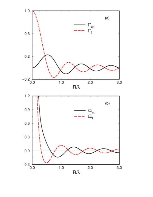
FIG. 3.: Plots of dd-coupling coefficients as a function of the atomic separation. Here $\theta=\pi/2$, i.e. both the atoms lie on the $xy$-plane and $\phi=\pi/4$. The new coherence terms $\Gamma_{vc}$, $\Omega_{vc}$ are comparable to $\Gamma_{i}$, $\Omega_{i}$. All the coefficients are scaled with $\gamma$.

Further, in Fig. 4 we examine the atomic position dependences of these coefficients. We have plotted the coupling coefficients as a function of $\phi$. Here we have fixed $\theta=\pi/2$; i.e. both the atoms are lying in the $xy$-plane. Again for a comparison, we have plotted $\Gamma_{1}$ and $\Gamma_{vc}$ in Fig. 4(a), and $\Omega_{1}$ and $\Omega_{vc}$ in Fig. 4(b). We observe the following special cases:

Case I: If $\theta=n\pi$, then $\Gamma_{vc}=\Omega_{vc}=0$; i.e. if $\vec{R}$ is perpendicular to the plane containing $\vec{d}_{1}$ and $\vec{d}_{2}$, the interference terms in the master equation drop out.

Case II: When $\phi=n\pi/2$, the coherence terms $\Gamma_{vc}=\Omega_{vc}=0$; i.e. when the second atom is placed in a position such that $\vec{R}$ is along one of the dipoles $\vec{d}_{1}$ or $\vec{d}_{2}$, then again the interference terms drop out. Thus the interference effects in the radiatively coupled systems are sensitive to the geometry.

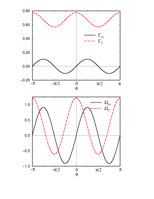
FIG. 4.: The dd-coupling terms as a function of the azimuthal angle $\phi$. Here $\theta=\pi/2$ and the atomic separation is taken to be $\lambda/4$. All coefficients are scaled with $\gamma$.

IV Numerical Results

In this section we present the numerical results that demonstrate the effect of the interference terms on the dynamics of the radiatively coupled multilevel systems. We use fifth order Runge-Kutta method for the numerical solution of the master equation (26). For numerical solutions we use the initial condition that at $t=0$, the first atom is in excited state $|1_{A}\rangle$ and the second atom is in the ground state $|3_{B}\rangle$.

In Fig. 5, we have plotted the density matrix element $\rho_{12}^{(A)}\equiv\langle 1_{A}|\langle 3_{B}|\rho(t)|2_{A}\rangle|3_{B}\rangle$ which represents the coherence in the excited states of atom $A$ when atom $B$ is in ground state $|3_{B}\rangle$. It is clear from Fig. 5 that the interference terms $\Gamma_{vc},~{}\Omega_{vc}$ in the master equation result in finite coherence in atom $A$. Otherwise, when $\Gamma_{vc}=\Omega_{vc}=0$, such coherences vanish. It is important to note that this coherence is produced by the radiative coupling between two atoms even when the dipole matrix elements $\vec{d}_{1}$ and $\vec{d}_{2}$ are orthogonal.

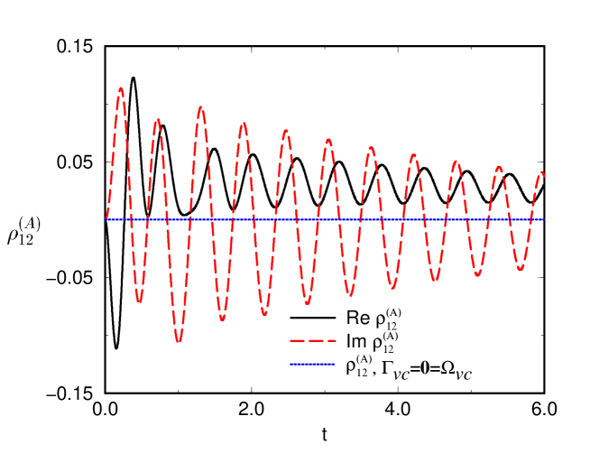
FIG. 5.: Time evolution of the coherence in the excited states of atom $A$ with atom $B$ being in $|3_{B}\rangle$. The coherence evolves only for non-zero values of $\Gamma_{vc}$ and $\Omega_{vc}$. Large oscillations are seen in $\rho_{12}^{(A)}$ which is decided by $\Omega_{i},~{}\Omega_{vc}$, and $\delta$. The parameters used are $\theta=\pi/2,~{}\phi=\pi/4,~{}R=\lambda/2\pi$ and $\delta=3\gamma$.

In Figs. [6-7], we plot the probabilities that atom $A$ is in state $|i_{A}\rangle$ and atom $B$ is in $|j_{B}\rangle$, which we denote by $p_{i;j}\equiv\langle i_{A}|\langle j_{B}|\rho(t)|i_{A}\rangle|j_{B}\rangle$. In Fig. 6(a), we present $p_{3;2}(t)$ that represents the simultaneous probability of atom $A$ being de-excited to state $|3_{A}\rangle$ and atom $B$ being excited to the state $|2_{B}\rangle$. Fig. 6(b) is the plot of $p_{2;3}(t)$ that represents the probability that the atom $A$ is excited to state $|2_{A}\rangle$ with atom $B$ being in $|3_{B}\rangle$. Obviously both $p_{3;2}$ and $p_{2;3}$ become zero if $\Gamma_{vc}=\Omega_{vc}=0$. It is observed that smaller the atomic separation larger is the excitation probability. For atomic separation $R=\lambda/2\pi$, the excitation probabilities are very large, e.g. more than $25\%$ of the population in atom $B$ could be excited to state $|2_{B}\rangle$ at $t\sim 0.3/\gamma$ (Fig. 6(a)) and, similarly in atom $A$, $\sim 18.5\%$ population could be excited to state $|2_{A}\rangle$ at $t\sim 0.5/\gamma$. Thus significant amount of energy transfer can take place between the states $|1_{A}\rangle$ and $|2_{B}\rangle$, though the corresponding transition dipoles are orthogonal to each other. Note that the initial evolution of $p_{2;3}$ is much slower compared to the evolution of $p_{3;2}$. This can be understood as follows: The excitation of atom $B$ to the state $|2_{B}\rangle$ can be caused by a single photon transfer from $A$ to $B$ [the process $|1_{A},3_{B}\rangle\rightarrow|3_{A},2_{B}\rangle$], whereas the excitation of atom $A$ to the state $|2_{A}\rangle$ occurs only through atom $B$ and this involves a net transfer of two photons [processes $|1_{A},3_{B}\rangle\rightarrow|3_{A},2_{B}\rangle\rightarrow|2_{A},3_{B}\rangle$ or $|1_{A},3_{B}\rangle\rightarrow|3_{A},1_{B}\rangle\rightarrow|2_{A},3_{B}\rangle$]. The oscillatory character of $p_{3;2}$ and $p_{2;3}$ comes from non-vanishing $\delta$ and from the dd-coupling co-efficients $\Omega_{i}$ and $\Omega_{vc}$. The excitation probabilities are seen to be larger for degenerate excited states ($\delta=0$) compared to that with finite separation between the excited states. For very large $\delta$ ($>>\gamma$), this interference effect disappears.

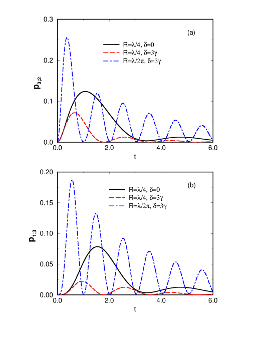
FIG. 6.: The time evolution of (a) $p_{3;2}$ and (b) $p_{2;3}$ are plotted for different parameters with the initial condition that atom $A$ is in state $|1_{A}\rangle$ and atom $B$ in $|3_{B}\rangle$. In both cases $\theta=\pi/2$ and $\phi=\pi/4$. The values of other parameters are shown as legends.

In Fig. 7, we present a comparative study of the probability that atoms remain in their initial states, i.e. $p_{1;3}$, in the presence and absence of the dd-coupling terms. The probability of atom $A$ staying in $|1_{A}\rangle$ decays exponentially in the absence of atom $B$. However, in the presence of the second atom, the nature of its decay is significantly modified - large oscillations are seen in $p_{1;3}$ in the presence of the new coherence terms, which is evident from Fig. 7. The origin of this oscillation is attributed to the large values of $\Omega_{vc}$.

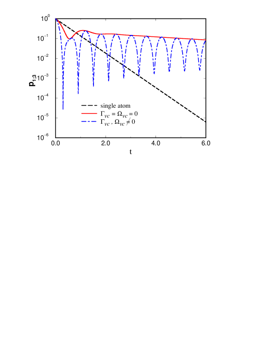
FIG. 7.: Plot of the probability that both atoms remain in their initial states. This probability is plotted on a logarithmic scale as a function of time in linear scale. The parameters used are $\theta=\pi/2,~{}\phi=\pi/4,~{}R=\lambda/4$ and $\delta=0$.

V Two $V$-systems with magnetic sub-levels in the presence of a magnetic field

In this section we consider the new coherence effects in two $V$-systems with $m$-degenerate magnetic sub-levels as excited states. The system could be, for example, a ⁴⁰Ca system - where $4~{}^{1}P_{1}$ degenerate sublevels would correspond to the excited states $|1_{\mu}\rangle\equiv|j=1,m=1\rangle$ and $|2_{\mu}\rangle\equiv|j=1,m=-1\rangle$, and the $4~{}^{1}S_{0}$ state would correspond to the ground state $|3_{\mu}\rangle$. In this case the dipole matrix elements $\vec{d}_{1}$ and $\vec{d}_{2}$ are complex and orthogonal to each other, and are given by

$$\vec{d}_{1}=-d\hat{\epsilon}_{-},~{}\vec{d}_{2}=d\hat{\epsilon}_{+};~{}\hat{\epsilon}_{\pm}=\frac{\hat{x}\pm i\hat{y}}{\sqrt{2}},$$ (48)

where $d$ is the reduced dipole matrix element. The magnetic field produces a Zeeman splitting $\delta$ and fixes the quantization axis ($z$ axis in our case). The geometry can be taken to be the same as in Fig. 2. However, in the present case, $\vec{d}_{1}$ and $\vec{d}_{2}$ being complex dipoles, they are not fixed along the real axes unlike in Fig. 2. Using Eq. (33), the dd coupling coefficients for this scheme can be obtained

$$\Gamma_{1} = \Gamma_{2}=\frac{|d|^{2}}{2\hbar}{\rm Im}~{}(\chi_{xx}+\chi_{yy})\equiv\frac{3\gamma}{4}(2P_{i}-\sin^{2}\theta Q_{i}),$$ (49)

$$\Omega_{1} = \Omega_{2}=\frac{|d|^{2}}{2\hbar}{\rm Re}~{}(\chi_{xx}+\chi_{yy})\equiv\frac{3\gamma}{4}(2P_{r}-\sin^{2}\theta Q_{r}),$$ (50)

$$\Gamma_{vc} = -\frac{|d|^{2}}{2\hbar}\left[{\rm Im}~{}(\chi_{xx}-\chi_{yy})+i~{}{\rm Im}~{}(\chi_{xy}+\chi_{yx})\right]\equiv\frac{3\gamma}{4}\sin^{2}\theta e^{2i\phi}Q_{i},$$ (51)

$$~{}~{}\Omega_{vc} = -\frac{|d|^{2}}{2\hbar}\left[{\rm Re}~{}(\chi_{xx}-\chi_{yy})+i~{}{\rm Re}~{}(\chi_{xy}+\chi_{yx})\right]\equiv\frac{3\gamma}{4}\sin^{2}\theta e^{2i\phi}Q_{r}.$$ (52)

The $P$s’ and $Q$s’ are as defined in Eq. (26). In deriving (52), we have used the fact that $\chi_{xy}=\chi_{yx}$. It may be noted that $\Gamma_{i}$ and $\Omega_{i}$ are real, and are independent of the azimuthal angle, whereas $\Gamma_{vc}$ and $\Omega_{vc}$ are complex and are functions of $\phi$. For $\theta=n\pi$, the coherence terms disappear in Eq. (26). Thus if $\vec{R}$ is perpendicular to the plane containing both the dipoles, i.e. both atoms lie on the quantization axis ($z$-axis), the coherence effects vanish.

The solutions of the master equation can be recalculated using the above coefficients and the analog of all the results presented in Sec.IV can be produced for the present system. For completeness, we present the numerical plot that shows the excitation probability $p_{3;2}$ with the initial condition $p_{1;3}(t=0)=1$. The time evolution of $p_{3;2}$ is similar to the one in the case of real dipoles (cf. Fig. 6(a)).

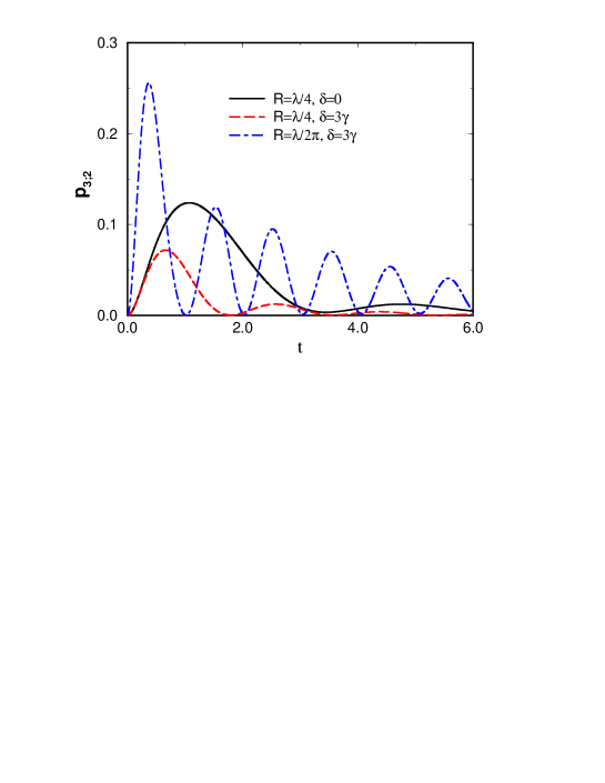
FIG. 8.: The time evolution of the probability $p_{3;2}$ when the dipoles $\vec{d}_{1}$ and $\vec{d}_{2}$ are complex. All the parameters are same as in Fig. 6.

It may further be noted that $p_{3;2}$ is independent of $\phi$ though $\Gamma_{vc}$ and $\Omega_{vc}$ are functions of $\phi$. This is because $p_{3;2}$ is a function of the absolute values of $\Gamma_{vc}$ and $\Omega_{vc}$. - which can be shown from (42) and (52), to the lowest order in $\Gamma_{vc}$ and $\Omega_{vc}$,

$$p_{3;2}\approx 4\left(|\Gamma_{vc}|^{2}+|\Omega_{vc}|^{2}\right)\left(\frac{\sin^{2}(\delta/2)}{\delta^{2}}\right).$$ (53)

We now discuss how the new coherence effect can be monitored experimentally for the above mentioned system. The dipole transitions $|1_{\mu}\rangle\leftrightarrow|3_{\mu}\rangle$, in the system described above, involve photons having $\sigma_{+}$ polarization. Thus the emission from $|1_{\mu}\rangle\rightarrow|3_{\mu}\rangle$ does not contain any field component in $\sigma_{-}$ polarization. On the other hand, the emission from $|2_{\mu}\rangle\rightarrow|3_{\mu}\rangle$ would contain $\sigma_{-}$ component. Thus the signal that one has to look for is - the intensity of the emitted photon from $|2_{\mu}\rangle$ levels in $\sigma_{-}$ polarization, which would a be measure of the total excitation probability to $|2_{\mu}\rangle$ states and hence would confirm the occurrence of VIC. Another possibility to probe the population in $|2_{\mu}\rangle$ will be to excite it with a circularly polarized radiation to a fourth state $6~{}^{1}S_{0}$ and to monitor the fluorescence from $6~{}^{1}S_{0}$.

VI Conclusions

In conclusion, we have shown that the radiative coupling between multilevel atoms with near-degenerate transitions can produce new interference effects which are especially important when the distance between two dipoles is less than a wavelength. We have demonstrated this possibility by considering two identical $V$-systems such that the pair of transition dipole matrix elements in each system are orthogonal to each other in both the atoms. Such interference effects are especially significant in the energy transfer studies. The choice of orthogonal dipole matrix elements enables us to specially isolate the effects of the vacuum induced coherences in the radiative coupling between multilevel atoms with nearly degenerate transitions. We have presented detailed numerical results to bring out the role of multi-atom multilevel interference effects.

REFERENCES

- [1] G. S. Agarwal, “Quantum Statistical Theories of Spontaneous Emission and their relation to other approaches”, Springer Tracts in Modern Physics: Quantum Optics (Springer-Verlag, 1974), Sec.15.
- [2] D. A. Cardimona, M. G. Raymer, and C. R. Stroud Jr., J. Phys. B15, 55 (1982);
- [3] P. Zhou, and S. Swain, Phys. Rev. Lett. 77, 3995 (1996); Phys. Rev. A 56, 3011 (1997).
- [4] S. Menon, and G. S. Agarwal, Phys. Rev. A 61, 013807 (2000).
- [5] S. Menon, and G. S. Agarwal, Phys. Rev. A 57, 4014 (1998).
- [6] A. Imamoğlu, and S. E. Harris, Opt. Lett. 14, 1344 (1989); S. E. Harris, Phys. Rev. Lett. 62, 1033 (1989); A. Imamoğlu, Phys. Rev. A 40, 2835 (1989).
- [7] P. Zhou, and S. Swain, Phys. Rev. Lett. 78, 832 (1997).
- [8] E. Paspalakis, S. -Q. Gong, and P. L. Knight, Opt. Commun. 152, 293 (1998); S. -Q. Gong, E. Paspalakis, and P. L. Knight, J. Mod. Opt. 45, 2433 (1998).
- [9] C. H. Keitel, Phys. Rev. Lett. 83, 1307 (1999).
- [10] G. C. Hegerfeldt, and M. B. Plenio, Phys. Rev. A 46, 373 (1992); ibid, 47, 2186 (1993); T. P. Altenmüller, Z. Physik D34, 157 (1995).
- [11] A. K. Patnaik, and G. S. Agarwal, J. Mod. Opt. 45, 2131 (1998); Phys. Rev. A59, 3015 (1999).
- [12] H. R. Xia, C. Y. Ye, and S. Y. Zhu, Phys. Rev. Lett. 77, 1032 (1996); A clear physical picture is given in: G. S. Agarwal, Phys. Rev. A 55, 2457 (1997).
- [13] S. Y. Zhu, R. C. F. Chan, and C. P. Lee, Phys. Rev. A 52, 710 (1995); S. Y. Zhu, and M. O. Scully, Phys. Rev. Lett. 76, 388 (1996); H. Lee, P. Polynkin, M. O. Scully, and S. Y. Zhu, Phys. Rev. A 55, 4454 (1997); H. Huang, S. -Y. Zhu, and M. S. Zubairy, Phys. Rev. A 55, 744 (1997); F. Li, S. -Y. Zhu, ibid, 59, 2330 (1999).
- [14] P. R. Berman, Phys. Rev. A 58, 4886 (1998).
- [15] M. A. G. Martinez, P. R. Herczfeld, C. Samuels, L. M. Narducci, and C. H. Keitel, Phys. Rev. A 55, 4483 (1997).
- [16] E. Paspalakis, and P. L. Knight, Phys. Rev. Lett. 81, 293, (1998); E. Paspalakis, C. H. Keitel, and P. L. Knight, Phys. Rev. A 58, 4868 (1998); application to loss free propagation of short pulse laser is reported in: E. Paspalakis, N. J. Kylstra, and P. L. Knight, Phys. Rev. Lett. 81, 293, (1998).
- [17] G. S. Agarwal, Phys. Rev. Lett. 84, 5500 (2000).
- [18] R. H. Dicke, Phys. Rev. 93, 99 (1954); for an excellent review on the subject, see: M. Gross and S. Haroche, Phys. Rep. 93, 303 (1982).
- [19] R. G. DeVoe, and R. G. Brewer, Phys. Rev. Lett. 76, 2049 (1996); the theory is discussed in: R. G. Brewer, Phys. Rev. Lett. 77, 5153 (1996).
- [20] P. Mataloni, E. De Angelis, and F. De Martini, Phys. Rev. Lett. 85, 1420 (2000).
- [21] G. V. Varda and G. S. Agarwal, Phys. Rev. A 45, 6721 (1992).
- [22] G. V. Varda and G. S. Agarwal, Phys. Rev. A 44, 7626 (1991); D. F. V. James, Phys. Rev. A 47, 1336 (1993).
- [23] Two 2-level atoms inside cavity is considered in: G. S. Agarwal, and S. Dutta Gupta, Phys. Rev. A 57, 667 (1998); excitation exchange between atoms (atomic separation ) giving rise to self interference of a single photon is discussed in: H. T. Dung and K. Ujihara, Phys. Rev. A 59, 2524 (1999); Phys. Rev. Lett. 84, 254 (2000); energy exchange leading to modification in spontaneous emission in a mono-layer is reported in: P. T. Worthing, R. M. Amos, and W. L. Barnes, Phys. Rev. A 59, 865 (1999).
- [24] Z. Ficek, Phys. Rev. A 44, 7759 (1991); Z. Ficek and R. Tanaś, Opt. Commun. 153, 245 (1998).
- [25] G. Kurizki, Phys. Rev. A 42, 2915 (1990); S. John and T. Quang, Phys. Rev. A 52, 4083 (1995); S. Bay, P. Lambropoulos, and K. Molmer, Opt. Commun. 132, 257 (1996).
- [26] G. M. Meyer, and G. Yeoman, Phys. Rev. Lett. 79, 2650 (1997); G. Yeoman, and G. M. Meyer, Phys. Rev. A 58, 2518 (1998); Similar situation in free space is discussed in T. Rudlph, and Z. Ficek, Phys. Rev. A 58, 748 (1998).
- [27] A. Beige and G. C. Hegerfeldt, Phys. Rev. A 59, 2385 (1999); S. U. Addicks, A. Beige, M. Dakna, and G. C. Hegerfeldt, quant-ph/0002093 and references there in.
- [28] G. Lenz and P. Meystre, Phys. Rev. A 48, 3365 (1993); E. V. Goldstein P. Pax, and P. Meystre, Phys. Rev. A 53, 2604 (1996); G. J. Yang, O. Zobay, and P. Meystre, Phys. Rev. A 59, 4012 (1999);
- [29] Static dd interaction has been important in earlier studies on collisional transfer of excitation from one atom to the other, e.g. see: W. R. Green, M. D. Wright, J. F. Young, and S. E. Harris, Phys. Rev. Lett. 43, 120 (1979).
- [30] M. E. Crenshaw, M. Scalora, and C. M. Bowden, Phys. Rev. Lett. 68, 911 (1992); C. M. Bowden and J. P. Dowling, Phys. Rev. A 47, 1247 (1993); M. E. Crenshaw and C. M. Bowden, Phys. Rev. Lett. 85, 1851 (2000).
- [31] M. Born and E. Wolf, Principles of Optics, 7th Edition (Cambridge University Press, 1999), Sec. 2.3.3.