Contradiction of Quantum Mechanics with Local Hidden Variables for Continuous Variable Quadrature Phase Amplitude Measurements

Abstract

We demonstrate a contradiction of quantum mechanics with local hidden variable theories for continuous variable quadrature phase amplitude (“position” and “momentum”) measurements, by way of a violation of a Bell inequality. For any quantum state, this contradiction is lost for situations where the quadrature phase amplitude results are always macroscopically distinct. We show that for optical realisations of this experiment, where one uses homodyne detection techniques to perform the quadrature phase amplitude measurement, one has an amplification prior to detection, so that macroscopic fields are incident on photodiode detectors. The high efficiencies of such detectors may open a way for a loophole-free test of local hidden variable theories.

In 1935 Einstein, Podolsky and Rosen ${}^{\cite[cite]{[\@@bibref{Number}{1}{}{}]}}$ presented an argument for the incompleteness of quantum mechanics. The argument was based on the validity of two premises: no action-at-a-distance (locality) and realism. Bell ${}^{\cite[cite]{[\@@bibref{Number}{2}{}{}]}}$ later showed that the predictions of quantum mechanics are incompatible with the premises of local realism (or local hidden variable theories). Experiments ${}^{\cite[cite]{[\@@bibref{Number}{3}{}{}]}}$ based on Bell’s result support quantum mechanics, indicating the failure of local hidden variable theories.

One feature appears characteristic of all the contradictions of quantum mechanics with local hidden variables studied to date. The measurements considered have discrete outcomes, for example being measurements of spin or photon number. By this we mean specifically that the eigenvalues of the appropriate system hermitian operator, which represents the measurement in quantum mechanics, are discrete.

In this paper we show how the predictions of quantum mechanics are in disagreement with those of local hidden variable theories for a situation involving continuous quadrature phase amplitude (“position” and “momentum”) measurements. By this we mean that the quantum predictions for the probability of obtaining results $x$ and $p$ for position and momentum (and various linear combinations of these coordinates) cannot be predicted by any local hidden variable theory. This is of fundamental interest since the original argument ${}^{\cite[cite]{[\@@bibref{Number}{1}{}{}]}}$ of Einstein, Podolsky and Rosen was given in terms of position and momentum measurements. The original state considered by Einstein, Podolsky and Rosen, and that produced experimentally in the realisation by Ou et al ${}^{\cite[cite]{[\@@bibref{Number}{4}{}{}]}}$ of this argument, gives probability distributions for $x$ and $p$ completely compatible with a local hidden variable theory.

Second we suggest a new macroscopic aspect to the proposed failure of local hidden variable theories for the case where one uses optical homodyne detection to realise the quadrature phase amplitude measurement ${}^{\cite[cite]{[\@@bibref{Number}{4,5}{}{}]}}$. The homodyne detection method employs a second “local-oscillator” field which combines with the original field to provide an amplification prior to photodetection. In these experiments then large field fluxes fall incident on highly efficient photodiode detectors, in dramatic contrast to the former photon-counting experiments. A microscopic resolution (in absolute terms) of this incident photon number is not necessary to obtain the violations with local hidden variables. This is in contrast to many previously cited macroscopic proposals ${}^{\cite[cite]{[\@@bibref{Number}{6}{}{}]}}$ for which it appears necessary to resolve the incident photon number to absolute precision in order to show a contradiction with local hidden variable theories.

The high efficiency of detectors available in this more macroscopic detection regime may provide a way to test local hidden variables without the use of auxiliary assumptions ${}^{\cite[cite]{[\@@bibref{Number}{2,7}{}{}]}}$ which have weakened the conclusions of the former photon counting measurements. This high intensity limit has not been indicated by previous works ${}^{\cite[cite]{[\@@bibref{Number}{8}{}{}]}}$ which showed contradiction of quantum mechanics with local hidden variables using homodyne detection, since these analyses were restricted to a very low intensity of “local oscillator” field.

We consider the following two-mode entangled quantum superposition state ^[9,10]:

$$|\Psi>=N\int_{0}^{2\pi}|r_{0}e^{i\varsigma}>_{A}|r_{0}e^{-i\varsigma}>_{B}d\varsigma$$ (1)

Here $N$ is a normalisation coefficient. The $|\alpha>_{A}$, where $\alpha=r_{0}e^{i\varsigma}$, is a coherent state of fixed amplitude $r_{0}=|\alpha|$ but varying phase $\varsigma$, for a system at a location $A$. Similarly $|\beta>_{B}$, where $\beta=r_{0}e^{-i\varsigma}$ and $r_{0}=|\beta|$, is a coherent state of fixed amplitude but varying phase for a second system at a location $B$, spatially separated from $A$. The quantum state (1) is potentially generated, from vacuum fields, in the steady state by nondegenerate parametric oscillation ${}^{\cite[cite]{[\@@bibref{Number}{10}{}{}]}}$ as modelled by the following Hamiltonian, in which coupled signal-idler loss dominates over linear single-photon loss.

$$H=i\hbar E(\hat{a}_{1}^{\dagger}\hat{b}_{1}^{\dagger}-\hat{a}_{1}\hat{b}_{1})+\hat{a}_{1}\hat{b}_{1}\hat{\Gamma}^{\dagger}+\hat{a}_{1}^{\dagger}\hat{b}_{1}^{\dagger}\hat{\Gamma}$$ (2)

The $\hat{a}_{1}^{\dagger}$ and $\hat{a}_{1}$, and $\hat{b}_{1}^{\dagger}$ and $\hat{b}_{1}$, are the usual boson creation and destruction operators for the two spatially separated systems (for example field modes) at locations $A$, and $B$, respectively. In many optical systems the $\hat{a}_{1}$ and $\hat{b}_{1}$ are referred to as the signal and idler fields respectively. Here E represents a coherent driving parametric term which generates signal-idler pairs, while $\hat{\Gamma}$ represents reservoir systems which give rise to the coupled signal-idler loss. The Hamiltonian preserves the signal-idler photon number difference operator $\hat{a}_{1}^{\dagger}\hat{a}_{1}$-$\hat{b}_{1}^{\dagger}\hat{b}_{1}$, of which the quantum state (1) is an eigenstate, with eigenvalue zero. We note the analogy here to the single mode “even” and “odd” coherent superposition states $N_{\pm}^{1/2}(|\alpha>\pm|-\alpha>)$ (where $\alpha$ is real and $N_{\pm}^{-1}=2(1\pm exp(-2|\alpha|^{2})$) which are generated by the degenerate form (put $\hat{a}_{1}=\hat{b}_{1}$) of the Hamiltonian (2). These states for large $\alpha$ are analogous to the famous “Schrodinger-cat” states ${}^{\cite[cite]{[\@@bibref{Number}{11}{}{}]}}$ and have been recently experimentally generated ${}^{\cite[cite]{[\@@bibref{Number}{12}{}{}]}}$.

Consider the experimental situation depicted in Figure 1. Measurements are made of the field quadrature phase amplitudes $X_{\theta}^{A}$ at location $A$, and $X_{\phi}^{B}$ at location $B$. Here we define $X_{\theta}^{A}=\hat{a}_{1}exp(-i\theta)+\hat{a}_{1}^{\dagger}exp(i\theta)$; and $X_{\phi}^{B}=\hat{b}_{1}exp(-i\phi)+\hat{b}_{1}^{\dagger}exp(i\phi)$. Where our system is a harmonic oscillator, we note that the angle choices $\theta$ (or $\phi$) equal to zero and $\pi/2$ will correspond to position and momentum measurements respectively. The result for the amplitude measurement $X_{\theta}^{A}$ is a continuous variable which we denote by $x$. Similarly the result of the measurement $X_{\phi}^{B}$ is a continuous variable denoted by $y$.

We formulate a Bell inequality test for the experiment depicted by making the simplest possible binary classification of the continuous results $x$ and $y$ of the measurements. We classify the result of the measurement to be $+1$ if the quadrature phase result $x$ (or $y$) is greater or equal to zero, and $-1$ otherwise. With many measurements we build up the following probability distributions: $P_{+}^{A}(\theta)$ for obtaining a positive value of $x$; $P_{+}^{B}(\phi)$ for obtaining a positive $y$; and $P_{++}^{AB}(\theta,\phi)$ the joint probability of obtaining a positive result in both $x$ and $y$.

If we now postulate the existence of a local hidden variable theory, we can write the probabilities $P_{\theta,\phi}(x,y)$ for getting a result $x$ and $y$ respectively upon the simultaneous measurements $X_{\theta}^{A}$ and $X_{\phi}^{B}$ in terms of the hidden variables $\lambda$ as follows.

$$P_{\theta,\phi}(x,y)=\int\rho(\lambda)\quad p_{x}^{A}(\theta,\lambda)p_{y}^{B}(\phi,\lambda)\quad d\lambda$$ (3)

The $\rho(\lambda)$ is the probability distribution for the hidden variable state denoted by $\lambda$, while $p_{x}^{A}(\theta,\lambda)$ is the probability of obtaining a result $x$ upon measurement at $A$ of $X_{\theta}^{A}$, given the hidden variable state $\lambda$. The $p_{y}^{B}(\phi,\lambda)$ is defined similarly for the results and measurement at $B$. The independence of $p_{x}^{B}(\theta,\lambda)$ on $\phi$, and $p_{y}^{B}(\phi,\lambda)$ on $\theta$ is a consequence of the locality assumption, that the measurement at $A$ cannot be influenced by the experimenter’s choice of parameter $\phi$ at the location $B$ (and vice versa)${}^{\cite[cite]{[\@@bibref{Number}{13}{}{}]}}$ . It follows that the final measured probabilities $P_{++}^{AB}(\theta,\phi)$ can be written in a similar form

$$P_{++}^{AB}(\theta,\phi)=\int\rho(\lambda)\quad p_{+}^{A}(\theta,\lambda)p_{+}^{B}(\phi,\lambda)\quad d\lambda$$ (4)

where we have simply $p_{+}^{A}(\theta,\lambda)=\int_{x\geq 0}p_{x}^{A}(\theta,\lambda)dx$, and similarly for $p_{+}^{B}(\phi,\lambda)$. It is well known that one can now deduce ${}^{\cite[cite]{[\@@bibref{Number}{2}{}{}]}}$ the following “strong” Bell-Clauser-Horne inequality.

$$S={{P_{++}^{AB}(\theta,\phi)-P_{++}^{AB}(\theta,\phi^{\prime})+P_{++}^{AB}(\theta^{\prime},\phi)+P_{++}^{AB}(\theta^{\prime},\phi^{\prime})}\over{P_{+}^{A}(\theta^{\prime})+P_{+}^{B}(\phi)}}\leq 1$$ (5)

The calculation of the quantum prediction for $S$ for the quantum state (1) is straightforward. We note certain properties of the distribution $P_{++}^{AB}(\theta,\phi)$: it is a function only of the angle sum $\chi=\theta+\phi$ so we can abbreviate $P_{++}^{AB}(\theta,\phi)=P_{++}^{AB}(\chi)$; $P_{++}^{AB}(\chi)=P_{++}^{AB}(-\chi)$; and the marginals satisfy $P_{+}^{A}(\theta)=P_{+}^{B}(\phi)=0.5$. Results for $S$ are shown in Figure 2, for the choice of measurement angles $\theta+\phi=\theta^{\prime}+\phi^{\prime}=-(\theta^{\prime}+\phi)=\pi/4,\theta+\phi^{\prime}=3\pi/4$ (for example put $\theta=0,\phi=-\pi/4,\theta^{\prime}=\pi/2$ and $\phi^{\prime}=-3\pi/4$). This choice allows the simplification $S=3P_{++}^{AB}(\pi/4)-P_{++}^{AB}(3\pi/4)$. It can be shown that for small $r_{0}$ (less than about $1.5$) this angle choice maximises $S$.

Violations of the Bell inequality, and hence contradiction with the predictions of local hidden variables, are indicated for $0.96\lesssim r_{0}\lesssim 1.41$, the maximum violation of $S\approx 1.0157\pm 0.001$ being around $r_{0}\approx 1.1$. This is a substantially smaller violation than obtained in the discrete case (where $S\approx 1.2$) of spin measurements, considered originally by Bell. The choice of Bell inequality and quantum state to give a violation may not be optimal, but nevertheless the possibility of a contradiction of quantum mechanics with local hidden variables is established.

We note that the violations are lost at large coherent amplitudes $r_{0}$. In this limit the quantum probability distributions for $x$ and $y$ show two widely separated peaks (as indicated by Figure 3), the $+1$ and $-1$ results of the measurement then corresponding to macroscopically distinct outcomes, resembling the “alive” and “dead” states of the “Schrodinger cat” ${}^{\cite[cite]{[\@@bibref{Number}{11}{}{}]}}$. We obtain asymptotic (large $r_{0}$) analytical forms for the probability distributions which allow a complete search for all angles. Results indicate no violations of the Bell inequality (5) possible.

In fact it can be demonstrated that, for any quantum state, there is no incompatibility with local hidden variables for the case where the quadrature phase amplitude results $x$ and $y$ only take on values which are macroscopically distinct. In this case, the addition of a noise term of order the standard quantum limit (this corresponds to a variance $\Delta^{2}x=1$) to the result of quadrature phase amplitude measurement will not alter the $+1$ or $-1$ classification of the result. Yet it can be shown that the quantum predictions for the results of such a noisy experiment are given by the quantum Wigner function $W(x_{0}^{A},x_{\pi/2}^{A},x_{0}^{B},x_{\pi/2}^{B})$ for the state (1), convoluted by the gaussian noise term $(1/4{\pi}^{2})\exp\left(-\left[{x_{0}^{A}}^{2}+{x_{\pi/2}^{A}}^{2}+{x_{0}^{B}}^{2}+{x_{\pi/2}^{B}}^{2}\right]/2\right)$. This new Wigner function is always positive ${}^{\cite[cite]{[\@@bibref{Number}{14}{}{}]}}$ and can then act as a local hidden variable theory which gives all the predictions in the truly macroscopic “dead” or “alive” classification limit.

An examination however of the homodyne method of measurement of the quadrature phase amplitudes reveals a macroscopic aspect to the experiment proposed here for optical fields. The optical realisation ${}^{\cite[cite]{[\@@bibref{Number}{4,5}{}{}]}}$ of the quadrature phase amplitude measurement (see Figure 1) involves local oscillator fields at $A$ and $B$, which we designate by the boson operators $\hat{a}_{2}$ and $\hat{b}_{2}$ respectively. The measurement of $X_{\theta}^{A}$ proceeds when the local oscillator field at $A$ is combined with the field $\hat{a}_{1}$ using a beam splitter to form two combined fields $\hat{c}_{\pm}=\left(\hat{a}_{2}\pm\hat{a}_{1}\exp(-i\theta)\right)/\sqrt{2}$. A variable phase shift $\theta$ allows choice of the particular observable to be measured. Direct detection, using two photodetectors, of the intensities $\hat{c}_{\pm}^{\dagger}\hat{c}_{\pm}$ of the combined fields and subtraction of the two resulting photocurrents results in measurement of $I_{D}=\hat{c}_{+}^{\dagger}\hat{c}_{+}-\hat{c}_{-}^{\dagger}\hat{c}_{-}=s_{\theta}^{A}$ where $s_{\theta}^{A}=\hat{a}_{2}^{\dagger}\hat{a}_{1}\exp(-i\theta)+\hat{a}_{2}\hat{a}_{1}^{\dagger}\exp(i\theta)$. In the limit where the local oscillator fields are very intense one may replace the boson operators $\hat{a}_{2}$ and $\hat{b}_{2}$ by classical amplitudes $E_{A}$ and $E_{B}$ respectively. Assuming $E_{A}=E_{B}=E$ where $E$ is real, we see that $s_{\theta}^{A}=EX_{\theta}^{A}$. The $X_{\phi}^{B}$ are measured similarly to $X_{\theta}^{A}$ using a second beam splitter (to give fields $\hat{d}_{\pm}=\left(\hat{b}_{2}\pm\hat{b}_{1}\exp(-i\phi)\right)/\sqrt{2}$) and pair of photodetectors, at location $B$.

The important point is that the local oscillator acts as an amplifier prior to detection, the operators $s_{\theta}^{A},\hat{c}_{\pm}^{\dagger}\hat{c}_{\pm}$ and $\hat{d}_{\pm}^{\dagger}\hat{d}_{\pm}$ being photon number operators which have a macroscopic scaling in the very intense local oscillator limit ${}^{\cite[cite]{[\@@bibref{Number}{15}{}{}]}}$. Thus in these experiments large intensities fall incident on the photodetectors, and it is not necessary to determine these photon numbers with a microscopic uncertainty in order to arrive at the conclusion that local hidden variable theories are invalid ${}^{\cite[cite]{[\@@bibref{Number}{16}{}{}]}}$. This is in contrast with the previous photon counting experiments, and also many previous macroscopic proposals for which it appears that an absolute resolution of the incident photon number is necessary in order to show failure of local hidden variables. Our result then opens possibilities for testing quantum mechanics against local hidden variable theories in a loophole-free way using very efficient photodiode detectors.

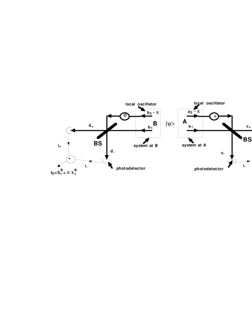
FIG. 1.: Schematic representation of a test of the Bell’s inequality. Balanced homodyne detection allows measurement of the quadrature phase amplitudes $X_{\theta}^{A}$ and $X_{\phi}^{B}$.

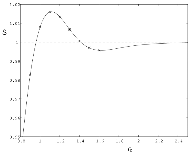
FIG. 2.: Plot of $S$ versus $r_{0}$, for the angle values indicated in the text.

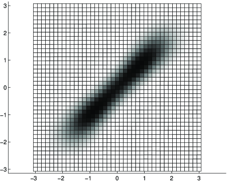
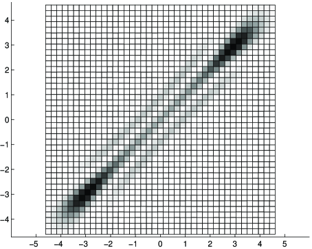
FIG. 3.: Representation of the quantum prediction for the probability $P_{\theta,\phi}(x,y)$ of getting a result $x$ (horizontal axis) and $y$ (vertical axis) respectively upon the simultaneous measurements $X_{\theta}^{A}$ and $X_{\phi}^{B}$, where $\theta=\phi$: (a) $r_{0}=1.1$; (b) $r_{0}=2.5$ showing the increasing separation of peaks and the interference fringes characteristic of quantum superposition states.

REFERENCES

- [1] A. Einstein, B. Podolsky and N. Rosen, Phys. Rev. 47, 777, (1935).
- [2] J. S. Bell, Physics, 1, 195, (19965). J. S. Bell, “Speakable and Unspeakable in Quantum Mechanics” (Cambridge Univ. Press, Cambridge, 1988). J. F. Clauser and M. A. Horne, Phys. Rev. D 10,526 (1974). J. F. Clauser and A. Shimony, Rep. Prog. Phys. 41, 1881 (1978), and references therein.
- [3] A. Aspect, P. Grangier and G. Roger, Phys. Rev. Lett. 49, 91, (1982). A. Aspect, J. Dalibard and G. Roger, ibid. 49, 1804, (1982). Y. H. Shih and C. O. Alley, Phys. Rev. Lett. 61, 2921, (1988). Z. Y. Ou and L. Mandel, Phys. Rev. Lett. 61, 50, (1988). J. G. Rarity and P. R. Tapster, Phys. Rev. Lett. 64, 2495, (1990). J. Brendel, E. Mohler and W. Martienssen, Europhys. Lett. 20, 575, (1992). P. G. Kwiat, A. M. Steinberg and R. Y. Chiao, Phys. Rev. A 47, 2472, (1993). T. E. Kiess, Y. H. Shih, A. V. Sergienko and C. O. Alley, Phys. Rev. Lett. 71 3893, (1993). P. G. Kwiat, K. Mattle, H. Weinfurter and A. Zeilinger, Phys. Rev. Lett. 75, 4337, (1995), D. V. Strekalov, T. B. Pittman, A. V. Sergienko, Y. H. Shih and P. G. Kwiat, Phys. Rev. A 54, 1, (1996).
- [4] Z. Y. Ou, S. F. Pereira, H. J. Kimble and K. C. Peng, Phys. Rev. Lett. 68, 3663 (1992).
- [5] H. P. Yuen and V. W. S. Chan, Opt. Lett. 8, 177 (1983).
- [6] N. D. Mermin, Phys. Rev. D 22, 356 (1980). P. D. Drummond, Phys. Rev. Lett. 50, 1407 (1983). A. Garg and N. D. Mermin, Phys. Rev. Lett. 49, 901 (1982). S. M. Roy and V. Singh, Phys. Rev. Lett. 67, 2761 (1991). A. Peres, Phys. Rev. A 46, 4413 (1992). M. D. Reid and W. J. Munro, Phys. Rev. Lett. 69, 997 (1992). G. S. Agarwal, Phys. Rev. A 47, 4608 (1993). D. Home and A. S. Majumdar, Phys. Rev. A 52, 4959 (1995). C. Gerry, Phys. Rev. A 54, 2529, (1996). N. D. Mermin, Phys. Rev. Lett. 65, 1838 (1990).
- [7] S. Pascazio, p 391 in “Quantum Mechanics versus Local Realism” ed. F. Selleri (Plenum Pub. Co., New York, 1988). E. Santos, Phys. Rev. A46,3646, (1992). M. Ferrero, T. W. Marshall and E. Santos, Am. J. Phys. 58, 683, (1990).
- [8] P. Grangier, M. J. Potasek and B. Yurke, Phys. Rev. A 38, 3132, (1988). B. J. Oliver and C. R. Stroud, Phys. Lett. A 135, 407, (1989). S. M. Tan, D. F. Walls and M. J. Collett, Phys. Rev. Lett. 66, 252, (1991). B. J. Sanders, Phys. Rev. A45, 6811, (1992).
- [9] G. S. Agarwal, Phys. Rev. Lett.57,827, (1986). K. Tara and G. S. Agarwal, Phys. Rev. A50, 2870, (1994).
- [10] M. D. Reid and L. Krippner, Phys. Rev. A47, 552, (1993).
- [11] E. Schrödinger, Naturwissenschaften 23, 812, (1935). A. J. Leggett and A. Garg, Phys. Rev. Lett. 54, 857 (1985).
- [12] C. Monroe, D. M. Meekhof, B. E. King and D. J. Wineland, Science, 272,1131, (1996). M. Brune, E. Hagley, J. Dreyer, X. Maitre, A. Maali, C. Wunderlich, J. M. Raimond and S. Haroche, Phys. Rev. Lett.77,4887, (1996). See also M. W. Noel and C. R. Stroud, Phys. Rev. Lett.77,1913, (1996).
- [13] As previously discussed in the literature (see A. Aspect, J. Dalibard and G. Roger, Phys. Rev. Lett 49, 1804, (1982); A. Zeilinger, Phys. Lett. A118, 1, (1986)) a stricter test is provided by ensuring measurement events at and are causally separated and that there is a sufficiently fast random switching between alternative choices of phase shift and , so that the locality condition follows from Einstein’s causality.
- [14] A. Peres, “Quantum Theory: Concepts and Methods”, (Kluwer Academic, Dordrecht, 1993).
- [15] M. D. Reid, Europhys. Lett. 36, 1 (1996). M. D. Reid Quantum Semiclass. Opt.9, 489, (1997).
- [16] Calculations reveal the violation of the Bell inequality to be sustained with only a very small ( ) amount of noise (lack of resolution) added to the result of the quadrature phase amplitude measurement of (or ). However because of the amplification, prior to photodetection, due to the local oscillator this small amount of noise in can in principle, for sufficiently large , translate to a large amount of noise (lack of resolution) in the detected photon number .