Macroscopic Local Realism Incompatible with Quantum Mechanics: Failure of Local Realism where Measurements give Macroscopic Uncertainties

Abstract

We show that quantum mechanics predicts a contradiction with local hidden variable theories for photon number measurements which have limited resolving power, to the point of imposing an uncertainty in the photon number result which is macroscopic in absolute terms. We show how this can be interpreted as a failure of a new premise, macroscopic local realism.

Bell ${}^{\cite[cite]{[\@@bibref{Number}{1}{}{}]}}$ in 1966 showed that the premises of local realism (or local hidden variable theories) were incompatible with the predictions of quantum mechanics. Experiments ${}^{\cite[cite]{[\@@bibref{Number}{2}{}{}]}}$ support quantum mechanics, and the general viewpoint is to reject the premise of local realism.

To date theoretical and experimental effort has focussed on situations where results of the relevant measurements need be only microscopically separated ${}^{\cite[cite]{[\@@bibref{Number}{15}{}{}]}}$. The measurements performed are intrinsically microscopic, in that one requires to clearly distinguish between results (eigenvalues of the appropriate quantum operator) which are microscopically distinct.

Theoretical work has shown a failure of local realism for multi-particle (or higher spin) systems ${}^{\cite[cite]{[\@@bibref{Number}{3}{}{}]}}$, where the system and range of results can be macroscopic. There have also been proposals ${}^{\cite[cite]{[\@@bibref{Number}{4}{}{}]}}$ which show failure of local realism for quantum superpositions of two macroscopically distinct states. However the violations are still apparently only indicated where measurements at some point must resolve microscopically different results, such as adjacent photon number or spin values. While the results indicate failure of local realism for macroscopic systems, it is not clear whether one is testing a premise different to that tested in the microscopic experiments.

Schrodinger ${}^{\cite[cite]{[\@@bibref{Number}{5}{}{}]}}$ raised the issue of quantum mechanics apparently predicting superpositions of states macroscopically distinct (“Schrodinger-cat states”), questioning the possibility of their true existence, based on the notion that such states apparently violate a type of macroscopic realism. Recent progress ${}^{\cite[cite]{[\@@bibref{Number}{6}{}{}]}}$ in the experimental generation of such superpositions highlights a need to test objectively for a true incompatibility with a macroscopic realism. Progress has been made by Leggett and Garg ${}^{\cite[cite]{[\@@bibref{Number}{7}{}{}]}}$ who predict an incompatibility of quantum mechanics with the premise of “macroscopic realism and noninvasive measurability”.

Here we define the premise of “macroscopic local realism” in such a way that its failure is more surprising than failure of the local realism addressed in previous Bell-type studies. This local realism becomes immediately testable in experiments where the results of all relevant measurements are macroscopically distinct, if a failure of local realism in the usual way can be shown. Experiments which still show a failure of local realism, even when uncertainties in all relevant measurements are macroscopic, will also show a failure of this type of macroscopic local realism. In this paper we prove this result and present a quantum state with this property, claiming therefore what is to our knowledge the first reported predicted failure of such macroscopic local realism.

In 1935 Einstein, Podolsky and Rosen ${}^{\cite[cite]{[\@@bibref{Number}{8}{}{}]}}$ defined “local realism” in the following way. “Realism” is sufficient to state that if one can predict with certainty the result of a measurement of a physical quantity at $A$, without disturbing the system $A$, then the results of the measurement were predetermined and one has an “element of reality” corresponding to this physical quantity. The element of reality is a variable which assumes one of a set of values which are the predicted results of the measurement. This value gives the result of the measurement, should it be performed. Locality states that the events at $A$ cannot, instantaneously, disturb in any way a second system at $B$ spatially separated from $A$. Taken together “local realism” is sufficient to imply that, if one can predict the result of a measurement of a physical quantity at $A$, by making a simultaneous measurement at $B$, then the result of the measurement at $A$ is described by an element of reality.

Macroscopic local realism ${}^{\cite[cite]{[\@@bibref{Number}{9}{}{}]}}$ is defined as a premise stating the following. If one can predict the result of a measurement at $A$ by performing a simultaneous measurement on a spatially separated system $B$, then the result of the measurement at $A$ is predetermined but described by an element of reality which has an indeterminacy in each of its possible values, so that only values macroscopically different to those predicted are excluded.

Macroscopic local realism is based on a “macroscopic locality”, which states that measurements at a location $B$ cannot instantaneously induce macroscopic changes (for example the dead to alive state of a cat, or a change between macroscopically different photon numbers) in a second system $A$ spatially separated from $B$. Macroscopic local realism also incorporates a “macroscopic realism”, since it implies elements of reality with (up to) a macroscopic indeterminacy. Suppose our “Schrodinger’s cat ${}^{\cite[cite]{[\@@bibref{Number}{5}{}{}]}}$” is correlated with a second spatially separated system, for example a gun used to kill the cat. The strength of macroscopic local realism is understood when one realises that its rejection in this example means we cannot think of the cat as being either dead or alive, even though we can predict the dead or alive result of “measuring” the cat, without disturbing the cat, by a measuring the correlated spatially-separated second system.

In this paper we present a quantum state which violates a Bell inequality even for coarse measurements with macroscopic uncertainties (in absolute terms), and show how this implies a failure of macroscopic local realism as we define it. Our proposed experiment is depicted in Figure 1a, where ($I_{0}$ is a modified Bessel function and $r_{0}=1.1$)

$$|\psi\rangle=[I_{0}(2r_{0}^{2})]^{-1/2}|\alpha>_{a_{+}}|\beta>_{b_{+}}\left(\sum_{n=0}^{\infty}\frac{(r_{0}^{2})^{n}}{n!}|{n}>_{a_{-}}|{n}>_{b_{-}}\right).$$ (1)

The $\hat{a}_{\pm}$ and $\hat{b}_{\pm}$ are boson operators for four outgoing fields. Fields $\hat{a}_{+}$ and $\hat{b}_{+}$ are in coherent states $|\alpha>_{a_{+}}$ and $|\beta>_{b_{+}}$ respectively, and we allow $\alpha$, $\beta$ to be real and large. $|{n}>_{k}$ is a Fock state for field $k$. The fields $\hat{a}_{-}$ and $\hat{b}_{-}$ are microscopic and are generated in a pair-coherent state ${}^{\cite[cite]{[\@@bibref{Number}{10}{}{}]}}$. Such states are the two-mode equivalent of the recently realised ${}^{\cite[cite]{[\@@bibref{Number}{6}{}{}]}}$ “even” and “odd” coherent superposition states ($(1\pm exp(-2|\alpha|^{2}))^{-1/2}(|\alpha>\pm|-\alpha>)/\sqrt{2}$) and could potentially be generated using nondegenerate parametric oscillation in a limit where one-photon losses are negligible. (The coherent states for $\hat{a}_{+}$ and $b_{+}$ would be derived from the laser pump for the oscillator.) We point out later other choices of $|\psi\rangle$ possible.

The fields $\hat{a}_{\pm}$ are mixed using phase shifts and beam splitters to give two new output fields $\hat{a}_{-}^{{}^{\prime}}=(\hat{a}_{-}-\hat{a}_{+})/\sqrt{2}$ and $\hat{a}_{+}^{{}^{\prime}}=i(\hat{a}_{-}+\hat{a}_{+})/\sqrt{2}$ at the location $A$. Similarly the fields $\hat{b}_{\pm}$ are mixed to give outputs $\hat{b}_{\pm}^{{}^{\prime}}$ at location $B$, spatially separated from $A$. The mixing is incorporated into the experiment simply to provide the nice feature that both fields, $\hat{a}_{\pm}^{{}^{\prime}}$ say at $A$, incident on the measuring apparatus are macroscopic. We measure simultaneously at $A$ and $B$ the Schwinger spin operators $\hat{S}_{\theta}^{A}=(\hat{c}_{+}^{\dagger}\hat{c}_{+}-\hat{c}_{-}^{\dagger}\hat{c}_{-})/2$ and $\hat{S}_{\phi}^{B}=(\hat{d}_{+}^{\dagger}\hat{d}_{+}-\hat{d}_{-}^{\dagger}\hat{d}_{-})/2$. The measurements are made through the transformations (achieved with polarisers or beam splitters with a variable transmission) $c_{+}=\hat{a}_{+}^{{}^{\prime}}\cos{\theta/2}+\hat{a}_{-}^{{}^{\prime}}\sin{\theta/2}$ and $c_{-}=\hat{a}_{+}^{{}^{\prime}}\sin{\theta/2}-\hat{a}_{-}^{{}^{\prime}}\cos{\theta/2}$, at $A$, and $d_{+}=\hat{b}_{+}^{{}^{\prime}}\cos{\phi/2}+\hat{b}_{-}^{{}^{\prime}}\sin{\phi/2}$ and $d_{-}=\hat{b}_{+}^{{}^{\prime}}\sin{\phi/2}-\hat{b}_{-}^{{}^{\prime}}\cos{\phi/2}$, at $B$, followed by photodetection.

In Figure 1b we demonstrate how the measurement $\hat{S}_{\theta}^{A}$ can also be performed directly from $\hat{a}_{\pm}$ by introducing a relative phase shift $\theta$ and mixing with a $50/50$ beam splitter to produce $\hat{c}_{\pm}^{{}^{\prime}}=\left(\hat{a}_{+}\pm\hat{a}_{-}\exp(-i\theta)\right)/\sqrt{2}$, followed by photodetection to give $\hat{S}_{\theta}^{A}=(\hat{c}_{+}^{{}^{\prime}\dagger}\hat{c}_{+}^{{}^{\prime}}-\hat{c}_{-}^{{}^{\prime}\dagger}\hat{c}_{-}^{{}^{\prime}})/2$.

Our test of macroscopic local realism requires noisy measurements. The result for the photon number differences $\hat{n}_{\theta}^{A}=2\hat{S}_{\theta}^{A}=\hat{c}_{+}^{\dagger}\hat{c}_{+}-\hat{c}_{-}^{\dagger}\hat{c}_{-}$ and $\hat{n}_{\phi}^{B}=2\hat{S}_{\phi}^{B}=\hat{d}_{+}^{\dagger}\hat{d}_{+}-\hat{d}_{-}^{\dagger}\hat{d}_{-}$ is of the form $n+noise$, where $n$ is the result of the measurement in the absence of the noise. We introduce noise distribution functions at each of $A$ and $B$, and define probabilities such as $P^{A}(noise\geq x)$, that the $noise$ at $A$ is greater than or equal to the value $x$. A probability $P^{B}(noise\geq x)$ is defined similarly. Later we allow $noise$ to be a random noise term with a gaussian distribution of standard deviation $\sigma$. Photon number measurements for macroscopic fields are performed with photodiode detectors, which already introduce a limited resolution because of detection inefficiencies.

The results of measurements are classified as $+1$ if the photon number difference result is positive or zero, and $-1$ otherwise. We determine the following probability distributions: $P_{+}^{A}(\theta)$ for obtaining $+$ at $A$; $P_{+}^{B}(\phi)$ for obtaining $+$ at $B$; and $P_{++}^{AB}(\theta,\phi)$ the joint probability of obtaining $+$ at both $A$ and $B$.

As a first step we define the probability $P_{ij}^{0,AB}(\theta,\phi)$ for obtaining results $i$ and $j$ respectively upon joint measurement of $\hat{n}_{\theta}^{A}$ at $A$, and $\hat{n}_{\phi}^{B}$ at $B$, in the absence of the applied noise $\sigma$. With noise present at the detectors, the measured probabilities $P_{++}^{AB}(\theta,\phi)$ become

$$P_{++}^{AB}(\theta,\phi)=\sum_{i,j=-\infty}^{\infty}P_{ij}^{0,AB}(\theta,\phi)P^{A}(noise\geq-i)P^{B}(noise\geq-j)$$ (2)

Before presenting the quantum prediction for these probabilities, we examine the prediction given by macroscopic local realism.

Local realism as originally defined by Einstein-Podolsky-Rosen, Bell and Clauser-Horne ${}^{\cite[cite]{[\@@bibref{Number}{1}{}{}]}}$ implies the following well known expression.

$$P_{ij}^{0,AB}(\theta,\phi)=\int\rho(\lambda)\quad p_{i}^{A}(\theta,\lambda)p_{j}^{B}(\phi,\lambda)\quad d\lambda$$ (3)

Local realism implies an underlying set of elements of reality, or hidden variables $\lambda$ (with probability distribution $\rho(\lambda)$), not specified by quantum theory. The element of reality is a variable which assumes one of a set of values which are the predicted results of the measurement, $\hat{n}_{\theta}^{A}$ say. For our experiment, a precise prediction of $\hat{n}_{\theta}^{A}$ is not possible given a measurement at $B$, for any choice $\phi$ at $B$. The elements of reality then do not take on definite values and local realism is only sufficient to imply a probability $p_{i}^{A}(\theta,\lambda)$ for the result $i$ of the measurement $\hat{n}_{\theta}^{A}$, for a given $\lambda$. The independence of $p_{i}^{A}(\theta,\lambda)$ on $\phi$ is based on the locality assumption.

Now we consider the prediction given by macroscopic local realism. With macroscopic local realism the locality condition is relaxed, but only up to the level of $M$ photons, where $M$ is not macroscopic, by maintaining that the measurement at $B$ cannot instantaneously change the result at $A$ by an amount exceeding $M$ photons. The elements of reality deduced using macroscopic local realism can give predictions for the results of measurement which are microscopically (or mesoscopically) different, but not macroscopically different, to those predicted from the elements of reality deduced using local realism. Where our predicted result at $A$ is $i^{{}^{\prime}}$ using local realism, macroscopic local realism allows the result to be $i=i^{{}^{\prime}}+m_{A}$ where $m_{A}$ can be any number not macroscopic. Importantly, while $i^{{}^{\prime}}$ is not dependent on the choice $\phi$ at $B$, the nonmacroscopic value $m_{A}$ can be. Where local realism specifies a (local) probability distribution $p_{i^{\prime}}^{A}(\theta,\lambda)$ for obtaining $i^{\prime}$ photons at $A$, the prediction is only correct to within $\pm M$ photons. The actual result at $A$ is determined by a further nonlocal perturbation term $p_{m_{A}}^{A}(i^{{}^{\prime}},{\theta,\phi},\lambda)$, which gives the probability of a further change of $m_{A}$ photons. The macroscopic local realism assumption then is that the conditional probability $p_{i}^{A}(\theta,\lambda)$ in equation (3) is expressible as the convolution (and similarly for $p_{i}^{B}(\phi,\lambda)$):

$$p_{i}^{A}({\theta,\phi},\lambda)=\sum_{m_{A}=-M}^{+M}p_{m_{A}}^{A}(i^{{}^{\prime}},{\theta,\phi},\lambda)p_{i^{\prime}=i-m_{A}}^{A}(\theta,\lambda).$$ (4)

The original local probability $p_{i^{\prime}}^{A}(\theta,\lambda)$ can be convolved with a microscopic nonlocal probability function $p_{m_{A}}^{A}(i^{{}^{\prime}},{\theta,\phi},\lambda)$, the only restriction being that the nonlocal distribution does not provide macroscopic perturbations, so that the probability of getting a nonlocal change outside the range $m_{A}=-M,...,+M$ is zero. Equivalently we must have (and similarly for terms with $B$)

$$\sum_{m_{A}=-M}^{M}p_{m_{A}}^{A}(i^{{}^{\prime}},{\theta,\phi},\lambda)=1.$$ (5)

We substitute the macroscopic locality assumption (4) into the hidden variable prediction (3) to obtain the prediction for the measured probabilities (2).

$$P_{++}^{AB}(\theta,\phi) = \sum_{i,j=-\infty}^{\infty}\int\rho(\lambda)\biggl{[}\sum_{m_{A}=-M}^{M}p_{m_{A}}^{A}(i^{{}^{\prime}},{\theta,\phi},\lambda)p_{i^{\prime}=i-m_{A}}^{A}(\theta,\lambda)\biggr{.}$$ (6)

$$\times \biggl{.}\sum_{m_{B}=-M}^{M}p_{m_{B}}^{B}(j^{{}^{\prime}},{\phi,\theta},\lambda)p_{j^{\prime}=j-m_{B}}^{B}(\phi,\lambda)\biggr{]}d\lambda\quad P^{A}(noise\geq-i)P^{B}(noise\geq-j)$$ (7)

Recalling $i=i^{\prime}+m_{A}$ and $j=j^{\prime}+m_{B}$ we change the $i$, $j$ summation to one over $i^{\prime}$, $j^{\prime}$ to get

$$P_{++}^{AB}(\theta,\phi) = \sum_{i^{\prime},j^{\prime}=-\infty}^{\infty}\int\rho(\lambda)p_{i^{\prime}}^{A}(\theta,\lambda)\biggl{[}\sum_{m_{A}=-M}^{M}p_{m_{A}}^{A}(i^{{}^{\prime}},{\theta,\phi},\lambda)P^{A}(noise\geq-(i^{\prime}+m_{A}))\biggr{]}\biggr{.}$$ (8)

$$\times p_{j^{\prime}}^{B}(\phi,\lambda)\biggl{[}\sum_{m_{B}=-M}^{M}\biggl{.}p_{m_{B}}^{B}(j^{{}^{\prime}},{\phi,\theta},\lambda)P^{B}(noise\geq-(j^{\prime}+m_{B}))\biggr{]}d\lambda$$ (9)

We assume that the noise function $noise$ is slowly varying over the microscopic (or mesoscopic) range $-m_{A},..+m_{A}$ for which nonlocal perturbations are possible according to macroscopic local realism (and similarly at $B$):

$$\sum_{m_{A}=-M}^{M}p_{m_{A}}^{A}(i^{{}^{\prime}},{\theta,\phi},\lambda)P^{A}(noise\geq-(i^{\prime}+m_{A}))\approx P^{A}(noise\geq-i^{\prime})\sum_{m_{A}=-M}^{M}p_{m_{A}}^{A}(i^{{}^{\prime}},{\theta,\phi},\lambda).$$ (11)

This is only valid if $\sigma$ is macroscopic. Using (5), one simplifies to get the final form $P_{++}^{AB}(\theta,\phi)=\sum_{i^{\prime},j^{\prime}}\ \int\rho(\lambda)p_{i^{\prime}}^{A}(\theta,\lambda)p_{j^{\prime}}^{B}(\phi,\lambda)d\lambda\times P^{A}(noise\geq-i^{\prime})P^{B}(noise\geq-j^{\prime})$. This prediction of the hidden variable theory is now given in a (local) form like that of (3), from which Bell- Clauser-Horne inequalities ${}^{\cite[cite]{[\@@bibref{Number}{1}{}{}]}}$ follow, for example:

$$S={{P_{++}^{AB}(\theta,\phi)-P_{++}^{AB}(\theta,\phi^{\prime})+P_{++}^{AB}(\theta^{\prime},\phi)+P_{++}^{AB}(\theta^{\prime},\phi^{\prime})}\over{P_{+}^{A}(\theta^{\prime})+P_{+}^{B}(\phi)}}\leq 1.$$ (12)

The noise terms which add a macroscopic uncertainty to the photon number result alter the premises needed to derive the Bell inequality. With $\sigma$ macroscopic we need only assume macroscopic local realism to derive the Bell inequality (9).

The quantum prediction for state (1) is shown in Figure 2. Violations of the Bell inequality (9) in the absence of $noise$ are shown in curve (a). Violations are still possible (curve (b)) in the presence of increasingly larger absolute noise $\sigma$, simply by increasing $\alpha=\beta$. This violation of the Bell inequality (9) with macroscopic noise $\sigma$ implies the failure of macroscopic local realism.

The asymptotic behavior in the large $\alpha$,$\beta$ limit is crucial in determining a violation of macroscopic local realism, and is best understood by replacing the boson operators $\hat{a}_{+}$ and $\hat{b}_{+}$ with classical amplitudes $\alpha$ and $\beta$ respectively. We see that then $\hat{S}_{\theta}^{A}=\alpha\hat{X}_{\theta}^{A}/2$ and $\hat{S}_{\phi}^{B}=\beta\hat{X}_{\phi}^{B}/2$, where $\hat{X}_{\theta}^{A}=\hat{a}_{-}exp(-i\theta)+\hat{a}_{-}^{\dagger}exp(i\theta)$ and $\hat{X}_{\phi}^{B}=\hat{b}_{-}exp(-i\phi)+\hat{b}_{-}^{\dagger}exp(i\phi)$ are the quadrature phase amplitudes of fields $\hat{a}_{-}$ and $\hat{b}_{-}$. In fact Figure 1b with $\alpha$,$\beta$ large shows the experimental set-up for balanced homodyne detection of the quadrature phase amplitudes $\hat{X}_{\theta}^{A}$ and $\hat{X}_{\phi}^{B}$, of fields $\hat{a}_{-}$ and $\hat{b}_{-}$. Homodyne detection has been used experimentally to detect ”squeezed” fields ${}^{\cite[cite]{[\@@bibref{Number}{11}{}{}]}}$, where the fluctuation in $\hat{X}_{\theta}^{A}$ is reduced below the standard quantum limit.

Violations of Bell inequalities for measurements $\hat{X}_{\theta}^{A}$, $\hat{X}_{\phi}^{B}$ on state (1) have recently been predicted ${}^{\cite[cite]{[\@@bibref{Number}{12}{}{}]}}$, confirming Figure 2(a) in the large $\alpha$ limit. These violations vanish ${}^{\cite[cite]{[\@@bibref{Number}{13}{}{}]}}$ when gaussian noise of standard deviation $\sigma_{0}\geq 0.26$ is added to the measurements $\hat{X}_{\theta}^{A},\hat{X}_{\phi}^{B}$. With $\alpha$ large, this corresponds to a noise value of $\alpha\sigma_{0}$ in the photon number measurement $2\hat{S}_{\theta}^{A}$, confirming Figure 2(b). In fact, since there is always a finite cutoff $\sigma_{0}$, any state $|\psi\rangle$ which shows a failure of local realism for measurements $\hat{X}_{\theta}^{A}$ and $\hat{X}_{\phi}^{B}$ on fields $\hat{a}_{-}$ and $\hat{b}_{-}$ will also show a violation of macroscopic local realism, provided $\alpha$,$\beta$ are large. Other such states have been recently predicted ${}^{\cite[cite]{[\@@bibref{Number}{14}{}{}]}}$, increasing the scope for a practical violation of macroscopic local realism.

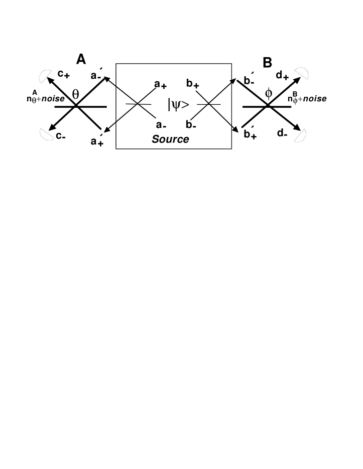
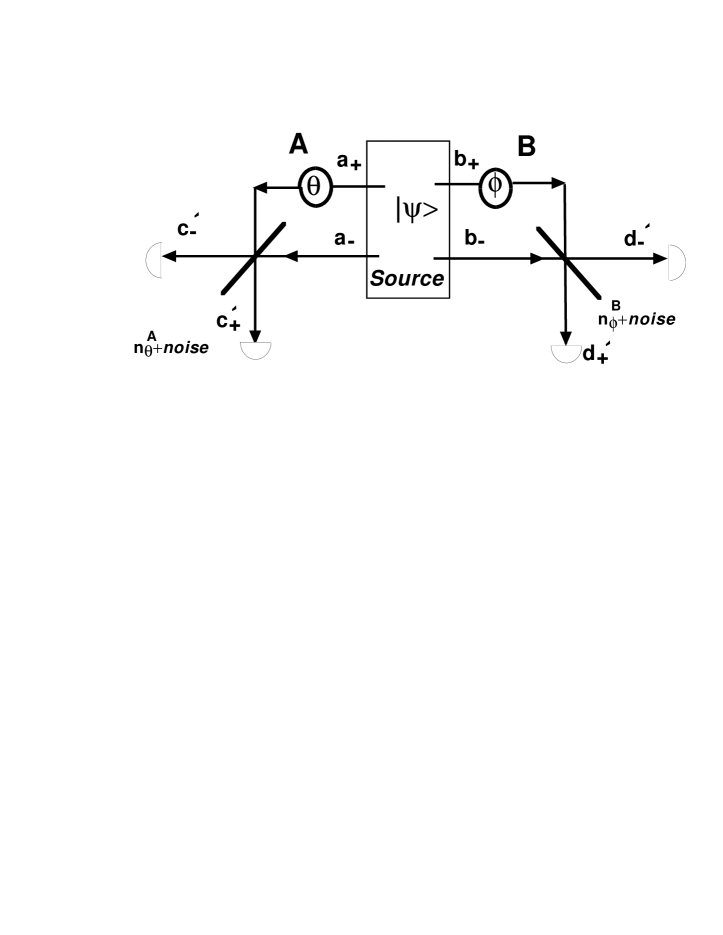
FIG. 1.: Our proposed test of macroscopic local realism. (a) For large $\alpha,\beta$ macroscopic fields $a_{\pm}^{{}^{\prime}}$ ($b_{\pm}^{{}^{\prime}}$) are incident on each measuring apparatus. (b) This measurement scheme for $\alpha,\beta$ large corresponds to balanced homodyne detection of the quadrature phase amplitudes $\hat{X}_{\theta}^{A}$ and $\hat{X}_{\phi}^{B}$.

FIG. 2.: (a) $S$ versus $\alpha=\beta$, for $\theta=0,\phi=-\pi/4,\theta^{\prime}=\pi/2,\phi^{\prime}=-3\pi/4$ for the quantum state (1) with no noise present. (b) Maximum noise $\sigma$ still giving a violation of the Bell inequality (9), versus $\alpha$.

REFERENCES

- [1] J. S. Bell, Physics, 1, 195, (1965). J. F. Clauser and A. Shimony, Rep. Prog. Phys. 41, 1881 (1978). D. M. Greenberger, M. Horne and A. Zeilinger, in “Bell’s Theorem, Quantum Theory and Conceptions of the Universe”, M.Kafatos, ed., Kluwer, Dordrecht, The Netherlands (1989), p. 69. N. D. Mermin, Physics Today 43 (6),9 (1990).
- [2] A. Aspect, P. Grangier and G. Roger, Phys. Rev. Lett. 49, 91, (1982). A. Aspect, J. Dalibard and G. Roger, ibid. 49, 1804, (1982). Y. H. Shih and C. O. Alley, Phys. Rev. Lett. 61, 2921, (1988). Z. Y. Ou and L. Mandel, Phys. Rev. Lett. 61, 50, (1988). J. G. Rarity and P. R. Tapster, Phys. Rev. Lett. 64, 2495, (1990). J. Brendel, E. Mohler and W. Martienssen, Europhys. Lett. 20, 575, (1992). P. G. Kwiat, A. M. Steinberg and R. Y. Chiao, Phys. Rev. A 47, 2472, (1993). T. E. Kiess, Y. H. Shih, A. V. Sergienko and C. O. Alley, Phys. Rev. Lett. 71, 3893, (1993). P. G. Kwiat, K. Mattle, H. Weinfurter, A. Zeilinger, A. Sergienko and Y. Shih, Phys. Rev. Lett. 75, 4337, (1995), D. V. Strekalov, T. B. Pittman, A. V. Sergienko, Y. H. Shih and P. G. Kwiat, Phys. Rev. A 54, 1, (1996). W. Gregor, T. Jennewein and A. Zeilinger, Phys. Rev. Lett. 81, 5039 (1998).
- [3] N. D. Mermin, Phys. Rev. D 22, 356 (1980). P. D. Drummond, Phys. Rev. Lett. 50, 1407 (1983). A. Garg and N. D. Mermin, Phys. Rev. Lett. 49, 901 (1982). S. M. Roy and V. Singh, Phys. Rev. Lett. 67, 2761 (1991). A. Peres, Phys. Rev. A 46, 4413 (1992). M. D. Reid and W. J. Munro, Phys. Rev. Lett. 69, 997 (1992). G. S. Agarwal, Phys. Rev. A 47, 4608 (1993). D. Home and A. S. Majumdar, Phys. Rev. A 52, 4959 (1995). C. Gerry, Phys. Rev. A 54, 2529, (1996).
- [4] N. D. Mermin, Phys. Rev. Lett. 65, 1838 (1990). B. J. Sanders, Phys. Rev. A45, 6811, (1992).
- [5] E. Schrödinger, Naturwissenschaften 23, 812, (1935). W. H. Zurek, Physics Today, 44, 36, (1991).
- [6] C. Monroe, D. M. Meekhof, B. E. King and D. J. Wineland, Science, 272,1131, (1996). M. Brune, E. Hagley, J. Dreyer, X. Maitre, A. Maali, C. Wunderlich, J. M. Raimond and S. Haroche, Phys. Rev. Lett.77,4887, (1996). M. W. Noel and C. R. Stroud, Phys. Rev. Lett.77,1913, (1996).
- [7] A. J. Leggett and A. Garg, Phys. Rev. Lett. 54, 857 (1985).
- [8] A. Einstein, B. Podolsky and N. Rosen, Phys. Rev. 47, 777, (1935). Z. Y. Ou, S. F. Pereira, H. J. Kimble and K. C. Peng, Phys. Rev. Lett. 68, 3663 (1992).
- [9] M. D. Reid, Europhys. Lett. 36, 1 (1996). M. D. Reid, Quantum Semiclass. Opt.9,489, (1997). M. D. Reid and P. Deuar, Ann. Phys. 265, 52 (1998).
- [10] G. S. Agarwal, Phys. Rev. Lett.57,827, (1986). M. D. Reid and L. Krippner, Phys. Rev. A47, 552, (1993).
- [11] H. P. Yuen and Shapiro,IEEE Trans. Inf. Theory 26,78 (1980).
- [12] A. Gilchrist, P. Deuar and M. D. Reid, Phys. Rev. Lett. 80, 3169 (1998); Phys. Rev. A, to be published.
- [13] P. Deuar, unpublished.
- [14] B. Yurke, M. Hillery and D. Stoler, quant-ph/9909042. W. J. Munro and G. J. Milburn, Phys. Rev. Lett. 81, 4285 (1998).
- [15] An exception is A. Peres, Found. Phys. 22,819 (1992).