Emergence of Fermi-Dirac Thermalization in the Quantum Computer Core

Abstract

We model an isolated quantum computer as a two-dimensional lattice of qubits (spin halves) with fluctuations in individual qubit energies and residual short-range inter-qubit couplings. In the limit when fluctuations and couplings are small compared to the one-qubit energy spacing, the spectrum has a band structure and we study the quantum computer core (central band) with the highest density of states. Above a critical inter-qubit coupling strength, quantum chaos sets in, leading to quantum ergodicity of eigenstates in an isolated quantum computer. The onset of chaos results in the interaction induced dynamical thermalization and the occupation numbers well described by the Fermi-Dirac distribution. This thermalization destroys the noninteracting qubit structure and sets serious requirements for the quantum computer operability.

I Introduction

The key ingredient of a quantum computer [1, 2] is that it can simultaneously follow all of the computation paths corresponding to the distinct classical inputs and produce a final state which depends on the interference of these paths. As a result, some computational tasks can be performed much more efficiently than on a classical computer. Shor [3] constructed a quantum algorithm which performs large number factorization into prime factors exponentially faster than any known classical algorithm. It was also shown by Grover [4] that the search of an item in an unstructured list can be done with a square root speedup over any classical algorithm. These results motivated a great body of experimental proposals for a construction of a realistic quantum computer (see [1, 2] and references therein). At present, quantum gates were realized with cold ions [5] and the Grover algorithm was performed for three qubits made from nuclear spins in a molecule [6]. For a proper operability, it is essential for the quantum computer to remain coherent during the computation process. Hence, a serious obstacle to its physical realization is the quantum decoherence due to the coupling with the external world [7, 8, 9]. In spite of that, in certain physical proposals, for example nuclear spins in two-dimensional semiconductor structures, the decoherence time can be many orders of magnitude larger than the time required for the gate operations (see for example Refs.[10, 11]). As a result, one can analyze the operation of an isolated quantum computer decoupled from the external world.

However, even if the quantum computer is isolated from the external world and the decoherence time is infinite, a proper operability of the computer is not guaranteed. As a matter of fact, one has to face a many-body problem for a system of $n$ interacting qubits (two level systems): any computer operation –a unitary transformation in the Hilbert space of size $N_{H}=2^{n}$– can be decomposed into two-qubit gates such as controlled-NOT and single qubit rotations [1, 2]. Due to the unavoidable presence of imperfections, the spacing between the two states of each qubit fluctuates in some detuning interval $\delta$. Also, some residual interaction $J$ between qubits necessarily remains when the two-qubit coupling is used to operate the gates.

In [12, 13, 14] an isolated quantum computer was modeled as a qubit lattice with fluctuations in individual qubit energies and residual short-range inter-qubit couplings. Similarly to previous studies of interacting many-body systems such as nuclei, complex atoms, quantum dots, and quantum spin glasses [15, 16, 17, 18, 19, 20, 21], the interaction leads to quantum chaos characterized by ergodicity of the eigenstates and level spacing statistics as in Random Matrix Theory [22]. The transition to chaos takes place when the interaction strength is of the order of the energy spacing between directly coupled states [15, 18, 19, 20, 21]. This border is exponentially larger than the energy level spacing in a quantum computer.

In this paper we show that the onset of chaos leads to occupation number statistics given by the Fermi-Dirac distribution. This means that a strong enough interaction plays the role of a heat bath, thus leading to dynamical thermalization for an isolated system. In such a regime, a quantum computer eigenstate is composed by an exponentially large (with $n$) number of noninteracting multi-qubit states representing the quantum register states. As a result, exponentially many states of the computation basis are mixed after a chaotic time scale and the computer operability is destroyed. We note that the dynamical thermalization has been discussed in other many-body interacting systems in [16, 17, 19, 23].

The paper is composed as follows. In Section II we describe our qubit lattice quantum computer model [12, 13, 14]; in Section III we discuss the statistical properties of the eigenvalues of this model; in Section IV we study the occupation number distribution and compare different definitions for the effective temperature of the system; the conclusions are presented in Section V.

II The model

We consider a model of $n$ qubits on a two-dimensional lattice with nearest neighbors inter-qubit coupling [24]. The Hamiltonian of this model, introduced in [12], reads:

$$H=\sum_{i}\Gamma_{i}\sigma_{i}^{z}+\sum_{i<j}J_{ij}\sigma_{i}^{x}\sigma_{j}^{x},$$ (1)

where the $\sigma_{i}$ are the Pauli matrices for the qubit $i$ and the second sum runs over nearest-neighbor qubit pairs on a two-dimensional lattice with periodic boundary conditions applied. The energy spacing between the two states of a qubit is determined by $\Gamma_{i}=\Delta_{0}+\delta_{i}$, with $\delta_{i}$ randomly and uniformly distributed in the interval $[-\delta/2,\delta/2]$. Therefore the detuning parameter $\delta$ gives the width of the $\Gamma_{i}$ distribution around its average value $\Delta_{0}$. For generality we choose the couplings $J_{ij}$, which represent the residual interaction, randomly and uniformly distributed in the interval $[-J,J]$. The model (1) can be considered as a standard generic quantum computer model, in which the unavoidable system imperfections generate a residual inter-qubit coupling and energy fluctuations. In a sense (1) describes the quantum computer hardware, while to study the gate operations in time one should include additional time-dependent terms in the Hamiltonian. At $J=0$, the noninteracting eigenstates of the model can be written as $|\psi_{k}\rangle=|\alpha_{1},...,\alpha_{n}\rangle$, where $\alpha_{i}=0,1$ marks the polarization of each individual qubit. These are the ideal multi-qubit eigenstates of a quantum computer, the quantum register states used for computer operations. For $J\neq 0$, these states are no longer eigenstates of the Hamiltonian, and the new multi-qubit eigenstates are now linear combinations of different quantum register states.

Here we focus on the case $\delta\ll\Delta_{0}$, which corresponds to the situation where fluctuations induced by imperfections are relatively weak [13]. In this case, the unperturbed energy spectrum of (1) (corresponding to $J=0$) is composed of $n+1$ well separated bands, with interband spacing $2\Delta_{0}$. Since the $\delta_{i}$ randomly fluctuate in an interval of size $\delta$, each band at $J=0$ (except the extreme ones) has a Gaussian shape of width $\approx\sqrt{n}\delta$ [25]. The average number of states inside a band $N_{B}$ is of the order of $N_{H}/n=2^{n}/n$, so that the energy spacing between adjacent multi-qubit states inside one band is exponentially small: $\Delta_{n}\sim n^{3/2}2^{-n}\delta$.

In the presence of a residual interaction $J\sim\delta$, the spectrum still has the above band structure with an exponentially large density of states. For $J,\delta\ll\Delta_{0}$, the interband coupling is very weak and can be neglected. In this situation, the Hamiltonian (1) is, to a good approximation, described by the renormalized Hamiltonian

$$H_{P}=\sum_{k=1}^{n+1}\hat{P_{k}}H\hat{P_{k}},$$ (2)

where $\hat{P_{k}}$ is the projector on the $k^{th}$ band, so that qubits are coupled only inside one band. We concentrate our studies on the central band. For an even $n$ this band is centered exactly at $E=0$, while for odd $n$ there are two bands centered at $E=\pm\Delta_{0}$, and we consider the one at $E=-\Delta_{0}$. The central band corresponds to the highest density of states, and in a sense represents the quantum computer core: an exponentially large number of states allows to take advantage of quantum parallelism in computer algorithms [1, 2, 3, 4]. On the other hand, quantum chaos and ergodicity first appear in this band, which therefore sets the limit for operability of the quantum computer. Inside this band, the system is described by the renormalized Hamiltonian $H_{P}$ which depends only on the number of qubits $n$ and the dimensionless coupling $J/\delta$.

III Spectral statistics

The results of Refs.[12, 13] showed that the quantum chaos border in (1) corresponds to a critical interaction $J_{c}$ given by:

$$J_{c}\approx\frac{C\delta}{n},$$ (3)

where $C$ is some numerical constant. This border is exponentially larger than the energy spacing between multi-qubit states $\Delta_{n}$. This is in agreement with previous studies of complex interacting many-body systems [15, 18, 19, 20, 21], in which the transition to quantum chaos takes place when the interaction matrix elements between directly coupled states become larger than their energy spacing. Since the interaction is of a two-body nature, each noninteracting multi-qubit state $|\psi_{k}\rangle$ has nonzero coupling matrix elements only with about $n$ other multi-qubit states. Therefore, the number of directly coupled states is much smaller than the number of multi-qubit states inside the central band, $N_{B}=n!/([n/2]!(n-[n/2])!)$ (we consider the band with the number of spins up given by the integer part of $n/2$). These couplings induce transitions in an energy interval of order $\delta$ (we assume that $J$ is of the order of or smaller than $\delta$). Therefore the energy spacing between directly coupled states is $\Delta_{c}\sim\delta/n$. The transition to chaos takes place for $J=J_{c}\approx\Delta_{c}$, which leads to the relation (3).

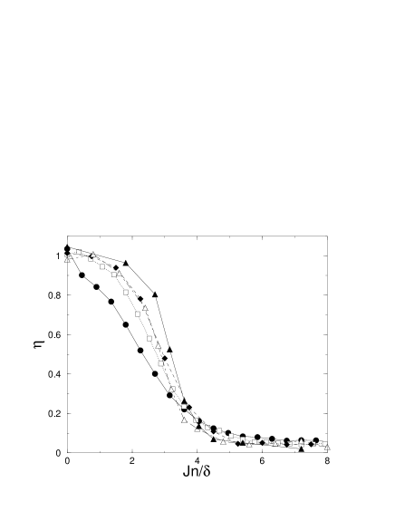
FIG. 1.: Dependence of $\eta$ on the scaled coupling $Jn/\delta$, for $n=9$ qubits (circles, $N_{D}=10^{4}$ random realizations of $\delta_{i},J_{ij}$), $n=12$ (squares, $N_{D}=10^{3}$), $n=15$ (diamonds, $N_{D}=45$), $n=16$ (empty triangles, $N_{D}=23$), and $n=18$ (filled triangles, $N_{D}=3$).The parameter $\eta$ is computed for $\pm 5\%$ of states around the center of the energy band.

The transition to quantum chaos and ergodic eigenstates can be detected in the change of the spectral statistics of the system. A convenient way is to look at the level spacing statistics $P(s)$, which gives the probability to find two adjacent levels whose spacing, normalized to the average level spacing, is in $[s,s+ds]$. In fact, $P(s)$ goes from the Poisson distribution $P_{P}(s)=\exp(-s)$ for nonergodic states to the Wigner-Dyson distribution $P_{W}(s)=(\pi s/2)\exp(-\pi s^{2}/4)$, corresponding to Random Matrix Theory, for ergodic states [22]. To analyze the change of $P(s)$ with the coupling $J$ one can conveniently use the parameter $\eta=\int_{0}^{s_{0}}(P(s)-P_{W}(s))ds/\int_{0}^{s_{0}}(P_{P}(s)-P_{W}(s))ds$ [19], where $s_{0}=0.4729...$ is the first intersection point of $P_{P}(s)$ and $P_{W}(s)$. In this way $P_{P}(s)$ corresponds to $\eta=1$ and $P_{W}(s)$ to $\eta=0$. Fig.1 gives the dependence of the parameter $\eta$ on the scaled coupling $Jn/\delta$ at different system sizes, for states near the middle of the energy spectrum ($\pm 5\%$ of levels around the band center). In order to reduce statistical fluctuations, we use $3\leq N_{D}\leq 10^{4}$ random realizations of $\delta_{i},J_{ij}$. In this way the total number of spacings $N_{S}$ is varied in the interval $1.4\times 10^{4}\leq N_{S}\leq 1.2\times 10^{5}$. The Poisson to Wigner-Dyson crossover becomes sharper when $n$ increases, suggesting a sharp transition in the thermodynamic limit. We note that, since the number of random $\delta_{i},J_{ij}$ values is not large, significant fluctuations are present in the $\eta$ curves when one changes the random realization. For example, for $n=18$, at $J=0.2\delta$, one has $\eta=0.44,0.29,0.06$ in the $N_{D}=3$ random realizations considered. This reflects the general property of fluctuations which become stronger near the critical transition point. On the other hand, even if the number of considered spacings is always large, for $n=15,16$ and especially for $n=18$, we have only a small number of random realizations, due to the very slow convergence of the Lanczos algorithm [26] near the band center, where the density of states becomes exponentially large. These fluctuations prevent us from precisely evaluating the critical scaled coupling for the Poisson to Wigner transition. The minimum spreading of curves is for $\eta(J_{c})\approx 0.2$, corresponding to $J_{c}n/\delta\approx 3.7$, in agreement with the results of Ref. [13]. We stress that the chaos border is exponentially larger than the multi-qubit level spacing, e.g., for $n=18$, $J_{c}\approx 0.2\delta\gg\Delta_{n}\approx 7\times 10^{-5}\delta$.

FIG. 2.: Level spacing statistics corresponding to Fig.1 at $n=16$, $J=0.05\delta$ (circles, $\eta=1.01$), $J=0.2\delta$ (triangles, $\eta=0.32$), and $J=0.4\delta$ (squares, $\eta=0.05$). Full curves show Poisson and Wigner-Dyson distributions.

The level spacing statistics near the band center is shown in Fig.2 at different coupling strengths $J$ for $n=16$. The transition from the Poisson to the Wigner-Dyson statistics is evident. In Fig.3 we show that, even away from the band center, the transition happens at approximately the same critical coupling. This is due to the fact that, even if the $n$-body density grows exponentially with the excitation energy, the density of coupled states remains roughly the same, except near the band edges [27]. We note that the data are shown only for half of the central band ($E<0$), since the density of states is symmetric around $E=0$ due to the presence of an upper bound in the single qubit energies.

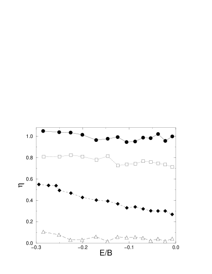
FIG. 3.: Dependence of $\eta$ on the energy $E$ (normalized to the total band width $B$ taken from numerical data) for $n=16$, $J=0.05\delta$ (circles), $J=0.15\delta$ (squares), $J=0.2\delta$ (diamonds), and $J=0.4\delta$ (triangles). Data are averaged over $N_{D}=15$ random realizations.

IV Dynamical thermalization

The transition in the level spacing statistics reflects a qualitative change in the structure of the eigenstates [12, 13]. While for $J\ll J_{c}$ the eigenstates are very close to the quantum register states, for $J>J_{c}$ each eigenstate $|\phi_{m}\rangle$ becomes a superposition of an exponentially large number of noninteracting eigenstates $|\psi_{k}\rangle$. It is convenient to characterize the complexity of an eigenstate $|\phi_{m}\rangle$ by the quantum eigenstate entropy

$$S_{q}=-\sum_{k=1}^{N_{B}}W_{km}\log_{2}W_{km},$$ (4)

where $W_{km}$ is the probability to find the quantum register state $|\psi_{k}\rangle$ in the eigenstate $|\phi_{m}\rangle$ of the Hamiltonian ($W_{km}=|\langle\psi_{k}|\phi_{m}\rangle|^{2}$). In this way $S_{q}=0$ if $|\phi_{m}\rangle$ is a quantum register state ($J=0$), $S_{q}=1$ if $|\phi_{m}\rangle$ is equally composed of two $|\psi_{i}\rangle$, and the maximum value is $S_{q}=\log_{2}N_{B}$ if all states equally contribute to $|\phi_{m}\rangle$.

Above the chaos border ($J>J_{c}$) one eigenstate is composed of order $2^{S_{q}}$ quantum register states, mixed inside the Breit-Wigner width $\Gamma\sim J^{2}/\Delta_{c}\sim J^{2}n/\delta$ [13]. As a result, the residual interaction disintegrates a quantum register state over an exponentially large number of states after a chaotic time scale $\tau_{\chi}\approx 1/\Gamma$ [13, 28]. After this time the quantum computer operability is certainly destroyed, unless one can apply quantum error-correcting codes (see [1, 2] and references therein) operating on a shorter time scale. This destruction takes place in an isolated system, without any external decoherence process. It happens due to inter-qubit coupling, which can mimic the effect of a coupling with the external world. In the following we show that in the quantum chaos regime a statistical description of our isolated $n$-qubit system is indeed possible, similarly to results found for other physical systems in [16, 17, 23].

We concentrate on the distribution of the occupation numbers $n_{i}$, defined as the probability that the qubit (spin) at the site $i$ is in its up polarization state. Given an eigenfunction $|\phi_{m}\rangle$ with eigenvalue $E_{m}$, one can write:

$$n_{i}(m)=\sum_{k=1}^{N_{B}}W_{km}\langle\psi_{k}|\hat{n}_{i}|\psi_{k}\rangle,$$ (5)

where $\hat{n}_{i}$ is the occupation number operator, and the term $\langle\psi_{k}|\hat{n}_{i}|\psi_{k}\rangle$ equals $1$ or $0$ depending on whether the spin at the site $i$ is up or down.

For noninteracting qubits one can write, e.g. for the central band,

$$\sum_{i=1}^{n}n_{i}(m)=\left[\frac{n}{2}\right],$$

$$\sum_{i=1}^{n}n_{i}(m)\delta_{i}=E_{m}^{{}^{\prime}},\quad(n_{i}(m)=0,1),$$ (6)

where $E_{m}^{{}^{\prime}}=E_{m}/2+\sum_{i}\delta_{i}/2$ ($E_{m}=\sum_{i}(2n_{i}(k)-1)\delta_{i}$). As $n_{i}(m)=0,1$, the relations (6) are the usual ones used to derive the Fermi-Dirac distribution for an ideal gas of many noninteracting particles in contact with a thermostat. However, here we consider an isolated system of relatively few interacting particles. Nevertheless, recent studies [16, 17, 23] have demonstrated that interaction can play the role of a heat bath, thus allowing one to use a statistical description even in an isolated system with few particles. The Fermi-Dirac statistics appears due to the fact that the number of spins up/down is fixed and in this way they become equivalent, for the purposes of a statistical description, to electrons/holes.

In Fig.4 we show the occupation number distribution, averaged over a few consecutive levels $|\phi_{m}\rangle$ and over $N_{D}=100$ random realization of $\delta_{i},J_{ij}$, for $n=16$ qubits, both in the integrable regime (top figures) and in the quantum chaos regime (bottom figures). We see that in both cases this averaged distribution is in very good agreement with the Fermi-Dirac distribution

$$n_{i}^{FD}=\frac{1}{\exp(\beta(\delta_{i}+\delta/2-\mu))+1},$$ (7)

where $\mu$ is the chemical potential and $\beta=1/T_{FD}$ is the inverse temperature (we set $k_{B}=1$). Taking into account the constraint set by the fixed number of spins up ($\sum_{i}n_{i}^{FD}=[n/2]$), $T_{FD}$ is the only fitting parameter.

The goodness of the fit given by the expression (7) is hardly surprising as statistical distributions are obtained for noninteracting particles after a correct counting of states. In this procedure, a weak interaction gives a slight increase of the system temperature [17].

A good agreement between the numerical data in Fig.4 and the theoretical distribution (7) does not mean that automatically there is equilibrium and thermalization for a given realization. This is outlined in Fig.5, which shows the occupation numbers for a single eigenstate of a given random realization. In the upper figures ($J=0.03\delta<<J_{c}\approx 0.2\delta$) a given eigenstate significantly projects only over a single quantum register state ($S_{q}<1$) and therefore half of the occupation numbers is close to $1$, half close to $0$, and the Fermi-Dirac distribution (7) is very far from the actual distribution. On the contrary, in the quantum chaos regime (lower figures, $J=0.3\delta>J_{c}$), where a large number of quantum register states are mixed in a single eigenstate, there is a good agreement between the occupation number distribution and the Fermi-Dirac distribution.

FIG. 4.: Distribution of the occupation numbers $n_{i}$ as a function of the qubit detunings $\delta_{i}$, for $n=16$ qubits, coupling strength $J=0.03\delta$ (upper figures) and $J=0.3\delta$ (lower figures), levels $m=5-10$ (left) and $m=95-100$ (right). Solid lines give Fermi-Dirac fits with effective temperature $T_{FD}$. Top left: $T_{FD}=0.13\delta$, mean excitation energy $\delta E=0.21\delta$, mean quantum eigenstate entropy $S_{q}=0.56$; top right: $T_{FD}=0.20\delta$, $\delta E=1.14\delta$, $S_{q}=0.81$; bottom left: $T_{FD}=0.17\delta$, $\delta E=0.24\delta$, $S_{q}=6.03$; bottom right: $T_{FD}=0.25\delta$, $\delta E=1.32\delta$, $S_{q}=8.04$. Data are averaged over $N_{D}=100$ random realizations.

In order to make quantitative the comparison with the Fermi-Dirac distribution, we introduce a parameter which measures the root mean square deviation of the actual distribution from (7):

$$\sigma_{FD}(m)=\sqrt{\frac{1}{n}\sum_{i=1}^{n}(n_{i}(m)-n_{i}^{FD}(m))^{2}.}$$ (8)

For the case of Fig.5, we have $\sigma_{FD}=6.3\times 10^{-2}$ (top left), $\sigma_{FD}=8.8\times 10^{-2}$ (top right) and much lower values above the chaos border: $\sigma_{FD}=1.4\times 10^{-2}$ (bottom left), $\sigma_{FD}=1.7\times 10^{-2}$ (bottom right). The maximum value $\sigma_{FD}^{max}=0.5$ is obtained at the band center ($T_{FD}=\infty$) for $J=0$, when $n_{i}=1$ for $[n/2]$ spins and $n_{i}=0$ for the remaining ones.

We introduce the thermalization border $J_{t}$ as follows: for $J<J_{t}$ eigenstates close in energy yield completely different $n_{i}$-distributions, for $J>J_{t}$ the $n_{i}$-distribution is stable with respect to the choice of a specific eigenstate in a small energy window. The appropriate quantity to be considered in addition to $\sigma_{FD}$ is the root mean square deviation of the occupation numbers for consecutive eigenstates:

$$\sigma_{s}=\sqrt{\frac{1}{n}\sum_{i=1}^{n}(n_{i}(m+1)-n_{i}(m))^{2}}.$$ (9)

For the case of Fig.5, we have $\sigma_{s}=0.1$ (top left), $\sigma_{s}=0.15$ (top right) and much lower values in the chaotic regime: $\sigma_{s}=2.9\times 10^{-2}$ (bottom left), $\sigma_{s}=3.3\times 10^{-2}$ (bottom right).

The conclusions drawn from Fig.5 are also applied to Fig.6 where, thanks to the effectiveness of the Lanczos algorithm [26] near the band edges, it was possible to consider a larger number of spins ($n=24$, corresponding to a very large Hilbert space dimension $N_{H}\approx 1.7\times 10^{7}$, with $N_{B}\approx 2.7\times 10^{6}$ levels in the central band).

FIG. 5.: Same as in Fig.4 but for a given random realization and a single eigenstate for $n=16$ qubits (left: $m=5$; right: $m=100$). Top left: $J=0.03\delta$, $T_{FD}=0.08\delta$, $\delta E=0.25\delta$, $S_{q}=0.23$; top right: $J=0.03\delta$, $T_{FD}=0.15\delta$, $\delta E=0.97\delta$, $S_{q}=0.49$; bottom left: $J=0.3\delta$, $T_{FD}=0.09\delta$, $\delta E=0.28\delta$, $S_{q}=5.85$; bottom right: $J=0.3\delta$, $T_{FD}=0.20\delta$, $\delta E=1.19\delta$, $S_{q}=8.41$.

Fig.7 shows the parameters $\sigma_{FD}$ and $\sigma_{s}$ as a function of the energy, for different values of the coupling strength $J$. As for the transition to chaos (Fig.3), the thermalization occurs at approximately the same critical coupling also away from the band center. We note that our data give $\sigma_{s}\approx\sqrt{2}\sigma_{FD}$, which can be easily understood as follows: $\sum_{i}(n_{i}(m+1)-n_{i}(m))^{2}\approx\sum_{i}(n_{i}(m)-n_{i}^{FD}(m))^{2}+\sum_{i}(n_{i}(m+1)-n_{i}^{FD}(m+1))^{2}-2\sum_{i}(n_{i}(m)-n_{i}^{FD}(m))(n_{i}(m+1)-n_{i}^{FD}(m+1))$, the last term in the sum becoming negligible after ensemble averaging. We stress that the very good agreement between the parameters $\sigma_{FD}$ and $\sigma_{s}$ implies that the Fermi-Dirac distribution emerges when the occupation number distribution is statistically stable, i.e. the system is thermalized. The curve for $J=0.05\delta$ lowers near the band edge since for a small excitation energy $\delta E$ a small number $n_{eff}\sim(n\delta E/\delta)^{1/2}$ of spins (“fermions”) is available for fluctuations in the vicinity of the Fermi level (see the note [27]).

FIG. 6.: Same as in Fig.5 but for $n=24$ qubits. Top left: $J=0.05\delta$, $T_{FD}=0.05\delta$, $\delta E=0.16\delta$, $S_{q}=0.51$; top right: $J=0.05\delta$, $T_{FD}=0.12\delta$, $\delta E=0.64\delta$, $S_{q}=1.84$; bottom left: $J=0.4\delta$, $T_{FD}=0.06\delta$, $\delta E=0.38\delta$, $S_{q}=7.75$; bottom right: $J=0.4\delta$, $T_{FD}=0.19\delta$, $\delta E=1.16\delta$, $S_{q}=12.55$.

It is interesting to compare the temperature $T_{FD}$ obtained from the Fermi-Dirac fit with different definitions of temperature [16, 17, 23], which are known to be equivalent at the thermodynamic limit. First of all we use the canonical expression

$$E(T_{can})=\frac{\displaystyle{\sum_{m=1}^{N_{B}}}E_{m}\displaystyle{\exp\left(-\frac{E_{m}^{\prime}}{T_{can}}\right)}}{\displaystyle{\sum_{m=1}^{N_{B}}}\displaystyle{\exp\left(-\frac{E_{m}^{\prime}}{T_{can}}\right)}},$$ (10)

where $E_{m}$ are the exact eigenenergies of the interacting system. The very good agreement between $T_{FD}$ and $T_{can}$ (see Fig.8) supports the validity of a statistical description for our isolated quantum computer model. This means that in such closed system the inter-qubit residual interaction plays the role of a heat bath in an open system. In particular, we expect that residual interaction mimics to a certain extent the effect of coupling to external world.

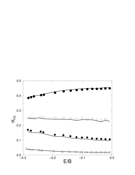
FIG. 7.: Root mean square deviation $\sigma_{FD}$ of the occupation number distribution with respect to the Fermi-Dirac fit as a function of the energy $E$ (normalized to the band width $B$), for $n=16$, $J=0.05\delta$ (circles), $J=0.15\delta$ (squares), $J=0.2\delta$ (diamonds), and $J=0.4\delta$ (triangles). Lines give $\sigma_{s}/\sqrt{2}$, with $\sigma_{s}$ root mean square deviation of the occupation numbers for consecutive levels. Data are averaged over $N_{D}=2$ random realizations.

FIG. 8.: Dependence of different definitions of temperature $T$ on the scaled energy $E/B$, for $n=16$, $J=0.3\delta$, $N_{D}=2$: $T_{FD}$ (circles), $T_{can}$ (full curve), and $T_{th}$ (dashed curve).

Finally we compare the effective temperature $T_{FD}$ with the standard thermodynamic temperature $T_{th}$, defined by

$$\frac{1}{T_{th}}=\frac{dS_{th}}{dE^{\prime}}=\frac{d\ln\rho}{dE^{\prime}},$$ (11)

where $S_{th}=\ln\rho$ is the thermodynamic entropy, with $\rho$ density of states (here $E^{\prime}$ replaces $E_{m}^{\prime}$). A Gaussian fit, $\rho=(1/\sqrt{2\pi}\sigma)\exp(-E^{\prime 2}/\sigma^{2})$, provides an excellent approximation to the actual data for the density of states, with the exception of the first few levels near the band edges. Therefore one gets $T_{th}=-\sigma^{2}/E^{\prime}$, with $\sigma^{2}$ variance of the Gaussian fit. Fig.8 shows that the difference between $T_{th}$ and $T_{FD}\approx T_{can}$ increases as one moves away from the band center. This is due to the fact that, contrary to the noninteracting case (see Eq.(6)), the actual system energy $E^{\prime}$ is different from $\sum_{i}n_{i}\delta_{i}$, since the total energy is renormalized due to interaction [17]. We remark that, not only on average but also for a single eigenstate of a given realization, the agreement between $T_{FD}$ and $T_{can}$ is good, while $T_{th}$ becomes closer to $T_{FD}$ and $T_{can}$ when the excitation energy increases. In the case of Fig.5 we obtain $T_{FD}=0.08\delta$, $T_{can}=0.07\delta$, $T_{th}=0.19\delta$ (top left), $T_{FD}=0.15\delta$, $T_{can}=0.16\delta$, $T_{th}=0.24\delta$ (top right), $T_{FD}=0.09\delta$, $T_{can}=0.08\delta$, $T_{th}=0.22\delta$ (bottom left), $T_{FD}=0.20\delta$, $T_{can}=0.19\delta$, $T_{th}=0.29\delta$ (bottom right). We also note that the effective temperature diverges at the band center and is negative in the upper part of the spectrum. This is typical of models with an upper bound in the single particle energies, in which the density of states has a maximum.

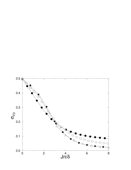
FIG. 9.: Dependence of $\sigma_{FD}$ on the scaled coupling $Jn/\delta$, for $n=9$ (circles, $N_{D}=2\times 10^{3}$ random realizations of $\delta_{i},J_{ij}$), $n=12$ (squares, $N_{D}=2\times 10^{2}$), $n=15$ (diamonds, $N_{D}=20$), and $n=16$ (triangles, $N_{D}=10$). The parameter $\sigma_{FD}$ is computed for $\pm 5\%$ of states around the band center. Transition to thermalization takes place at $J_{t}n/\delta\approx 3.2$.

The dependence of the thermalization parameter $\sigma_{FD}$ on the scaled coupling $Jn/\delta$ at different system sizes is shown in Fig.9 (very similar results are obtained for $\sigma_{s}/\sqrt{2}$). Our data show that the crossover to a thermalized distribution sharpens when the number of qubits increases, in a way consistent with a sharp thermalization border in the thermodynamic limit, at $J_{t}n/\delta\approx 3.2$. The similarity between the results of Fig.1 ($J_{c}n/\delta\approx 3.7$) and Fig.9 leads us to the conclusion that the chaos border coincides with the thermalization border. This looks quite natural since the Poisson level spacing statistics indicates the existence of uncoupled parts in the whole system, thus preventing thermalization. On the contrary, in the chaotic regime each eigenfunction spreads over an exponentially large number $N\approx 2^{S_{q}}$ of quantum register states, resulting in the Wigner-Dyson statistics. In this regime the fluctuations of eigenstate components are Gaussian [17] and therefore, according to the central limit theorem, the fluctuations of the occupation numbers are small: $\Delta n_{i}\propto N^{-1/2}\ll 1$. For this reason eigenstates close in energy give similar $n_{i}$-distributions, which means that there is equilibrium in the statistical sense.

V Conclusions

The results presented in this paper show that the residual inter-qubit coupling can lead to quantum chaos and a statistical description of the occupation numbers in close agreement with the Fermi-Dirac distribution. We stress that the transition to quantum chaos is an internal process which happens in a perfectly isolated system with no coupling to the external world. Nevertheless, the thermalization which appears in this closed system due to inter-qubit coupling can mimic the effect of an external thermal bath. Above the chaos/thermalization border the quantum register states are destroyed after the chaotic time scale and therefore serious restrictions are set to the quantum computer operability. However, below this border the imperfection effects only slightly disturb the ideal multi-qubit states and the quantum computer can operate properly in this regime.

We thank Bertrand Georgeot for stimulating discussions, and the IDRIS in Orsay and the CICT in Toulouse for access to their supercomputers.

REFERENCES

- [1] A. Steane, Rep. Progr. Phys. 61, 117 (1998).
- [2] The Physics of Quantum Information, edited by D. Bouwmeester, A. Ekert, and A. Zeilinger (Springer-Verlag, Berlin, 2000).
- [3] P. Shor, in Proceedings of the -th Annual Symposium on Foundations of Computer Science, edited by S. Goldwasser (IEEE Computer Society Press, Los Alamitos, CA, 1994), p. 124.
- [4] L.K. Grover, Phys. Rev. Lett. 79, 325 (1997); ibid. 80, 4329 (1998).
- [5] C. Monroe, D.M. Meekhof, B.E. King, W.M. Itano, and D.J. Wineland, Phys. Rev. Lett. 75, 4714 (1995).
- [6] L.M.K. Vandersypen, M. Steffen, M.H. Sherwood, C.S. Yannoni, G. Breyta, and I.L. Chuang, Appl. Phys. Lett. 76, 646 (2000).
- [7] J.I. Cirac and P. Zoller, Phys. Rev. Lett. 74, 4091 (1995).
- [8] C. Miquel, J.P. Paz, and R. Perazzo, Phys. Rev. A 54, 2605 (1996).
- [9] C. Miquel, J.P. Paz, and W.H. Zurek, Phys. Rev. Lett. 78, 3971 (1997).
- [10] D.P. Di Vincenzo, Science 270, 255 (1995).
- [11] D. Mozyrsky, V. Privman, and I.D. Vagner, cond-mat/0002350.
- [12] B. Georgeot and D.L. Shepelyansky, Phys. Rev. E 62, 3504 (2000).
- [13] B. Georgeot and D.L. Shepelyansky, quant-ph/0005015, Phys. Rev. E (in press).
- [14] D.L. Shepelyansky, quant-ph/0006073.
- [15] S. Åberg, Phys. Rev. Lett. 64, 3119 (1990).
- [16] M. Horoi, V. Zelevinsky, and B.A. Brown, Phys. Rev. Lett. 74, 5194 (1995); V. Zelevinsky, B.A. Brown, N. Frazier, and M. Horoi, Phys. Rep. 276, 85 (1996).
- [17] V.V. Flambaum, F.M. Izrailev, and G. Casati, Phys. Rev. E 54, 2136 (1996); V.V. Flambaum and F.M. Izrailev, Phys. Rev. E 56, 5144 (1997).
- [18] D.L. Shepelyansky and O.P. Sushkov, Europhys. Lett. 37, 121 (1997).
- [19] Ph. Jacquod and D.L. Shepelyansky, Phys. Rev. Lett. 79, 1837 (1997).
- [20] D.Weinmann, J.-L. Pichard, and Y. Imry, J. Phys. I France 7, 1559 (1997).
- [21] B. Georgeot and D.L. Shepelyansky, Phys. Rev. Lett. 81, 5129 (1998).
- [22] For a review see, e.g., T. Guhr, A. Müller-Groeling, and H.A. Weidenmüller, Phys. Rep. 299, 189 (1998).
- [23] F. Borgonovi, I. Guarneri, F.M. Izrailev, and G. Casati, Phys. Lett. A 247, 140 (1998).
- [24] We consider a two dimensional lattice for the sake of generality. In fact, the corresponding one-dimensional model can be mapped by the Wigner-Jordan transformation into a system of noninteracting fermions and therefore it is always integrable, see for example A.P. Young, Phys. Rev. B 56, 11691 (1997).
- [25] The majority of states are inside this interval, while, for the bands near to the center, the total band width is . This is due to rare events in the sum of random numbers.
- [26] J. Cullum and R.A. Willoughby, J. Comp. Phys. 44, 329 (1981).
- [27] At in the ground states the spins of lowest are up, the remaining ones are down. Then the low energy excitations (magnons) exchange the polarizations of a couple of qubits with energies close to the effective Fermi energy . Following standard estimates [19], the number of effectively interacting qubits at a temperature is given by , with excitation energy with respect to the -qubit ground state. This changes the chaos border (3) to .
- [28] V.V. Flambaum, quant-ph/9911061.