Understanding Spin: the field theory of magnetic interactions.

Abstract

Spin is commonly thought to reflect the true quantum nature of microphysics. We show that spin is related to intrinsic and field-like properties of single particles. These properties change continuously in external magnetic fields. Interactions of massive particles with homogeneous and inhomogeneous fields result in two discrete particle states, symmetric to the original one. We analyze the difficulties in quantum mechanics to give a precise spacetime account of the experiments and find that they arise from unsuitable analogies for spin. In particular from the analogy of an angular momentum. Several experiments are suggested to check the model against the standard model in quantum mechanics.

PACS numbers: 03.65.D,04.20.Gz

]

I Analogies and understanding

It has frequently been stressed that the mathematical form of quantum physics can be deduced from group theoretical considerations [1, 2]. A case was then made, that the linearity of quantum mechanics (= validity of superposition), together with the necessary symmetry operations, provides a full understanding of the theory. Even though this is true for a mathematician, it is not necessarly true for a physicist. The work of a mathematician is done, when the work of a physicist only begins. Let us call this part of theoretical physics, which differs from pure mathematical reasoning, understanding the physical theory. Understanding, in this sense, means a clear conceptual picture, why an entity must be described the way it is described, why these descriptions operate, the way they operate, and why they lead to the results they provide.

One of the most useful logical figures in understanding physics is the analogy. A difficult phenomenon is, via analogy, referred to a less difficult and more easily understandable one. The drawback of analogies is, they are not determined by logical necessity. Note that we use this term rather than the mathematically more precise mapping because of its connotations. While mapping only means that a series of experimental results can be mapped onto a theoretical model, a suitable analogy equals a consistent description of the physical processes involved. The two terms differ in their epistemological implications: whereas analogy is related to realism, mapping implies an essentially positivist view. For this reason we prefer analogy. We shall argue, in this paper, that the usual analogies for spin are wrong. Spin should be understood as something, the evaluation procedure in quantum mechanics does to the mathematical representation of a system. Incidentally a point, Bohr would have subscribed [3]. But we shall also describe the physical qualities of single particles, acted upon by external magnetic fields. And give a precise spacetime picture of the evolution of a particle’s magnetic properties. A description, commonly denied in standard frameworks.

The analogy for spin is based, like most analogies in quantum mechanics, on classical mechanics and electrodynamics. In particular, as we will prove, on a misleading combination of both to understand magnetic properties of matter. It is derived from the magnetic moment of current distributions in electrodynamics [4]. A current carrying loop, placed into a magnetic field, experiences a force along the field gradient. This force is proportional to the magnetic moment of the current loop. The implicit concept below the mathematical derivation of this force is the concept of Ampere’s molecular currents. In case of single particles the current carrying loop is replaced by the mechanical picture of a point charge in orbit around a defined center. This is the reason that in the original papers spin was usually called the ”spin angular momentum”.

With this analogy in mind Stern and Gerlach [5] performed experiments on the magnetic moment of silver atoms. The results did not agree with the simple classical picture. So they concluded that the simple classical picture, based on the described analogy, must be wrong. The answer to this problem, in the view of quantum mechanics, was given by Goudsmit and Uhlenbeck [6, 7]: the electron possesses an intrinsic angular momentum, which reveals itself in these measurements via its magnetic moment. This answer was generalized into an impressive mathematical formalism, not least by Pauli [8]. It is still the main answer, physicists accept as ultimately true. The problem, though, which remained, is the understanding of this intrinsic angular momentum. All attempts to refer it to some motion of a structured particle with a point-like charge did not convincingly remove the objection that this rotation seemingly has no direction in space. Then how can it be a rotation? (for a review of electron models trying to establish spin on this basis see [9]).

At this point we have two possibilities: (i) Either leave it at that and accept the numerical recipes as useful. (ii) Try to create a different, more suitable analogy. Which is, trying to understand spin. Even though the first approach has been employed in the past, the author does not consider it, ultimately, a physical approach: it leaves the problem of interpretation aside and thus is no more than mathematics. It is not enough for physics.

Quite generally, the approach to physics in the last, the 20th century, to leave all problems of interpretation aside and focus on mathematics alone, is inefficient. Because then only one route remains to new insights: mathematical intuition. Given that this is the most formal and hence least versatile intuition in terms of human imagination, the procedure in itself is questionable. Considering, in addition, that a precise image of a process can cover, within instants, developments it takes major computational efforts to reproduce numerically, the whole idea of a natural science based only on mathematical structures seems utterly absurd. All considered, it is not quite as absurd as that, because mathematical consistency has the advantage of greater generality. But there is a limit, as Aristotle remarked some two thousand years ago: the most general concepts are also the emptiest. And the ultimate structure of mathematical physics, the most general theory, will be devoid of any meaning. All it will cover is the structure of mathematics itself. This is quite compatible with the basic assumption in what became known as the Copenhagen Interpretation [10]: there is no independent reality.

In this paper we will base a theory of magnetic interactions on just such an independent reality, the intrinsic and field-like properties of single particles. In section II we shall briefly review the theoretical foundations of the treatment. Section III treats the interaction of neutral particles (neutrons, but also atoms) with homogeneous and inhomogeneous magnetic fields. Then, in section IV we shall briefly discuss measurements and statistics, while section V establishes an actual meaning of the spin concept in quantum mechanics.

II Foundations of Microdynamics

The theoretical framework in this paper is based on a strongly objective [11] theory of microphysics. Strong objectivity means that the entities we deal with in microphysics are assumed to have a reality and properties, which are completely independent of any measurement. These entities exist separate from any description, and even though their qualities change in interactions (that is, what we call a measurement), the qualities as such prevail also without measurements. In this sense the theory gives a definite answer to Mermin’s question [12]: ” Is the moon there when nobody looks?”, and the answer is: Yes, certainly.

The theory has its foundations in the intrinsic properties of moving particles. It was called, for obvious reasons, the Theory of Microdynamics (MD) [13]. Magnetic interactions and the analysis of spin will be treated from the viewpoint of the MD model of particles [14]. The main features of this model are (see Fig. 1):

• Particles are extended structures, the actual extension (= the volume of the particle) is usually irrelevant. This feature is due to the mathematical structure based on local differential equations.

• Particles are described by their intrinsic features alone: the variables of the description are mass density $\rho({\bf r},t)$, frequency $\nu$, the longitudinal momentum density ${\bf p}({\bf r},t)$, and the transversal intrinsic fields ${\bf E}({\bf r},t)$ and ${\bf B}({\bf r},t)$.

• The development of these intrinsic properties is governed by linear field equations connecting the variables.

• Scalar fields and dynamics of particle propagation are related via the concept of dynamic charge [15]. This concept is similar in spirit to the harmonic oscillator in quantum mechanics, but it remains firmly within a continuous and field theoretical framework.

FIG. 1.: The intrinsic fields of a particle in motion. The particle is extended over a volume $V$, which is not specified. The longitudinal velocity ${\bf u}$ and momentum density ${\bf p}$ are perpendicular to the transversal intrinsic fields ${\bf E}$ and ${\bf B}$.

The intrinsic fields and their properties are not statistical features of single particles, but essentially deterministic. The statistical ensembles, which also in MD arise in experiments, have two origins [16]:

• They are an expression of limited control of the experimental conditions. In the same sense as e.g. in the de Broglie-Bohm theory [17], the phase of intrinsic fields of a single particle is in general unknown.

• The ensembles are also an expression of limited knowledge about the interaction. From the viewpoint of MD also electrodynamics is a statistical theory [14]. This means that fields in electrodynamics have components interacting with a particle’s field-like properties, and components, interacting with its kinetic properties. A way to describe these (separate) components is using real and imaginary fields [18].

The equations necessary for the presentation will be stated in later sections. It should be noted that standard quantum mechanics (the Schrödinger equation) as well as standard electrodynamics (the Maxwell equations) can be referred to the field equations of intrinsic particle properties [14]. Therefore the treatment is general in terms of both theories. As will be seen presently, it allows an analysis of interaction processes from a field theoretical point of view and still recovers the essential results of quantum mechanics. In this sense the whole concept is well beyond a purely statistical interpretation of quantum mechanics and in fact a hidden variable theory. The hidden variables, in this theory, are the intrinsic fields and densities.

III Interaction of fermions with magnetic fields

A Homogeneous fields

We consider the motion of a beam of neutral particles in a homogeneous magnetic field. The trajectory of the particles is not affected. But recombining this beam with a reference beam not subjected to the magnetic field shows a changed interference pattern [19, 20] (see Fig. 2). The question is: why?

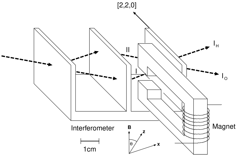
FIG. 2.: Neutron interferometer according to Rauch [20]. The coherent Neutron beam is split at the first lobe and recombined after the third. A magnetic field is applied to one partial beam (I). The effect is a shift of the interference pattern after recombination.

The particles are neutral, therefore an interaction between the external magnetic field and particle charge is excluded. The change of properties then must be due to intrinsic features not readily observed in standard experiments. In the conventional model this intrinsic feature is the spin of a particle, e.g. a neutron (half-spin) or photon (integer spin). In most textbooks spin is treated as a somewhat abstract variant of angular momentum (see e.g. [21]). This concept can be traced back to the original papers by Uhlenbeck and Goudsmit, where the authors concluded that [6]:

Das Elektron rotiert um seine eigene Achse mit dem Drehimpuls $\hbar/2$. Für diesen Wert des Drehimpulses gibt es nur 2 Orientierungen für den Drehimpulsvektor.

The obvious objection, that in macroscopic systems no angular momentum is known with just two orientations in space has been brushed aside with the remark, that this is due to the ”quantum nature” of spin. What the difference between this ”quantum nature” of the ”spin angular momentum” and the realistic nature of a macrophysical angular momentum actually is, has never been conclusively explained. And, as recent research revealed (see the introduction), it cannot be explained in a manner consistent with experimental facts. In this context it should be noted that the explanation of spin 1/2 by the Dirac equation is not correct. Because, as Gottfried and Weisskopf pointed out [22]:

At one time it (the Dirac equation) was thought to ’explain’ the spin s = 1/2 of the electron, but we now know that this is not so. Equations of the Dirac type can be constructed for any s. At this time we have no understanding of the remarkable fact that the fundamental fermions of particle physics … all have spin 1/2.

The model of extended particles does not provide a model of spin in its usual sense, all that exists are transversal intrinsic fields, called electromagnetic fields for convenience. The fields obey the Maxwell equations, the relevant equations are the following [14]:

$$\frac{1}{u^{2}}\frac{\partial{\bf E}({\bf r},t)}{\partial t}=\nabla\times{\bf B}({\bf r},t)$$ (1)

$$\qquad-\frac{\partial{\bf B}({\bf r},t)}{\partial t}=\nabla\times{\bf E}({\bf r},t)$$ (2)

$$\phi_{EM}({\bf r},t)=\frac{1}{2}\left(\frac{1}{u^{2}}{\bf E}^{2}({\bf r},t)+{\bf B}^{2}({\bf r},t)\right)$$ (3)

Here $u$ is the velocity of the particle and $\phi_{EM}$ the energy density of the electromagnetic field. We assume that the particle moves along $x$, the electromagnetic fields shall initially be polarized along the $y$ and $z$ axis of our coordinate system.

$${\bf E}({\bf r},t)=(0,E_{0},0)e^{i(k_{0}x-\omega_{0}t)}$$ (4)

$${\bf B}({\bf r},t)=(0,0,B_{0})e^{i(k_{0}x-\omega_{0}t)}$$ (5)

We consider the change of intrinsic fields due to an external magnetic field $B_{ext}$. The dynamic changes of the field environment, when the particle approaches the magnet are simulated by a finite interval $\tau$ taken for the field to be fully switched on. The field vector of the external field shall be:

$${\bf B}_{ext}=(0,-\sin\vartheta,\cos\vartheta)B_{ext}$$ (6)

For a linear increase of the field during $t\in[0,\tau]$ the internal fields at $\tau$ will be:

$$E^{\prime}_{y} = E_{0}e^{i(k_{0}x-\omega_{0}t)}-B_{ext}\cos\vartheta\frac{x}{\tau}$$ (7)

$$E^{\prime}_{z} = -B_{ext}\sin\vartheta\frac{x}{\tau}$$ (8)

$$B^{\prime}_{y} = -B_{ext}\sin\vartheta$$ (9)

$$B^{\prime}_{z} = B_{0}e^{i(k_{0}x-\omega_{0}t)}+B_{ext}\cos\vartheta$$ (10)

The amplitudes of the electromagnetic fields are related by [14]:

$$E_{0}=u_{0}B_{0}$$ (11)

Then the change of the electromagnetic energy density due to the external magnetic field is given by:

$$\delta\,\phi_{EM}(\tau,x)=\frac{1}{2}\left(\frac{B_{ext}^{2}}{u_{0}^{2}}\,\frac{x^{2}}{\tau^{2}}+B_{ext}^{2}\right)$$ (12)

One key feature of this new model of particles is the relation between mass oscillations (or changes of the density of mass) and scalar fields. The relation is described by the differential equation [15]:

$$\triangle\phi({\bf r},t)+\frac{\partial^{2}\rho({\bf r},t)}{\partial t^{2}}=0$$ (13)

In this one-dimensional case the integration of the equation is straightforward and the result obtained for the changed density of mass $\delta\rho$ and kinetic energy density $\delta\phi_{K}=\delta\rho u^{2}$ amounts to:

$$\delta\rho(\tau) = -\frac{1}{2}\frac{B_{ext}^{2}}{u_{0}^{2}}$$ (14)

$$\delta\phi_{K}(\tau) = \delta\rho(\tau)\cdot u_{0}^{2}=-\frac{1}{2}B_{ext}^{2}$$ (15)

In general electromagnetic fields must be described by complex vectors. This feature derives from the simultaneous existence of field components and kinetic components of particle energy. A thorough account of it will be given at the end of this section. Denoting the real and the imaginary part of the magnetic field by:

$$B^{+}=\Re(B_{ext})\quad B^{-}=\Im(B_{ext})\quad|B^{+}|=|B^{-}|=B_{E}$$ (16)

we get for the change of the kinetic energy density in a magnetic field the two symmetric solutions:

$$\delta\phi_{K}^{\pm}(\tau)=\mp\,\frac{1}{2}B_{E}^{2}$$ (17)

The intrinsic fields of the particle and the changes due to the interaction with the magnetic field are shown in Fig. 3. This change affects the two contributions to the energy, the field components and the kinetic components, in opposite ways. The total energy of the particle remains unchanged. This is, incidentally, also a requirement of electrodynamics. The requirement is not fulfilled in quantum mechanics. A fact, which so far seems to have escaped wider notice. Because strictly speaking it contradicts the field equations of electromagnetic fields.

Quite generally, the energy of a particle in a magnetic field is conserved. This is a consequence of the Lorentz force equation:

$${\bf F}_{L}=q{\bf v}\times{\bf B}\qquad dW={\bf F}_{L}d{\bf r}$$ (18)

$${\bf F}_{L}\perp\frac{d{\bf r}}{dt}\Rightarrow dW=0$$ (19)

If energy is transferred at all to the particle, then the medium of transfer must be the magnetic field. From the energy integral:

$$W_{B}\propto\int{\bf B}^{2}\,d^{3}r$$ (20)

it follows that this can only be accomplished by a change of the field itself:

$$\triangle W_{B}\propto\int_{R}(\triangle{\bf B})^{2}\,d^{3}r$$ (21)

where $R$ is the region of interaction. This requires that the absolute value and not only the the direction of the field changes due to the interaction. Which is only possible, if there is a drain of the field in the same region. And this, in turn, contradicts the source equations of magnetic fields:

$$\nabla{\bf B}=0$$ (22)

Therefore any transfer of energy from the field to the particle is not possible within the framework of electrodynamics. In other words, the QM concept of spin violates the energy principle in all cases, where it predicts a change of particle energy due to magnetic fields.

In the current treatment the magnetic field only changes the distribution between the two energy components. The changes of the energy distribution of the particle result from the dynamic changes of the field environment. In this sense a constant field does no longer affect the particle’s motion. This constant field is equal to the second term in equation (12). Taking consequently only the first term of Eq. (12) we get for the components and the total change of energy density of the particle:

$$\delta\phi_{EM}^{\pm}(\tau) = \pm\frac{1}{2}B_{E}^{2}$$ (23)

$$\delta\phi_{K}^{\pm}(\tau) = \mp\frac{1}{2}B_{E}^{2}$$ (24)

$$\delta\phi_{T}(\tau) = \delta\phi_{EM}(\tau)+\delta\phi_{K}(\tau)=0$$ (25)

The change of the particle’s density of mass does not leave the dynamic properties of motion unaffected. In particular the phase velocity in the magnetic field will be changed. This can be shown using the continuity equation:

$$\frac{\partial\rho({\bf r},t)}{\partial t}+\nabla{\bf p}({\bf r},t)=0$$ (26)

At an arbitrary point (x,t) along the change of the external field the changes of $\rho$, density of mass, and $u$, phase velocity of the particle’s wave (which is equal, in this model, to the mechanical velocity), are described by:

$$\rho(t) = \rho_{0}+\delta\rho(t)=\rho_{0}-\frac{1}{2}\frac{B_{ext}^{2}}{u_{0}^{2}}\cdot\frac{t^{2}}{\tau^{2}}$$ (27)

$$u(x) = u_{0}+\delta u(x)$$ (28)

Omitting terms of second order the changes are consequently:

$$\frac{\partial\delta\rho(t)}{\partial t}=-\rho_{0}\frac{\partial\delta u(x)}{\partial x}$$ (29)

Integrating we get for the change of the phase velocity at an arbitrary point (x,t):

$$\rho_{0}\delta u(x,t)=-\int_{0}^{x}dx^{\prime}\frac{\partial\delta\rho(t)}{\partial t}=\frac{1}{2}\frac{B_{ext}^{2}}{u_{0}^{2}}\frac{xt}{\tau^{2}}$$ (30)

And at the moment $t=\tau$, with $x=x_{1}$ and $x_{1}/\tau\approx u_{0}$ this amounts to:

$$u_{0}\delta u(\tau)\approx\frac{1}{2}\delta\,u^{2}(\tau)=\frac{1}{2}\,\frac{B_{ext}^{2}}{\rho_{0}}$$ (31)

Again, generalizing the expression for complex fields we obtain two symmetric solutions for the phase velocity in the magnetic field. The velocity difference, and thus the phase shift in the field is linear with the amplitude $B_{E}$ [20]:

$$\delta u(\tau)=\pm\frac{B_{E}}{\sqrt{\rho_{0}}}$$ (32)

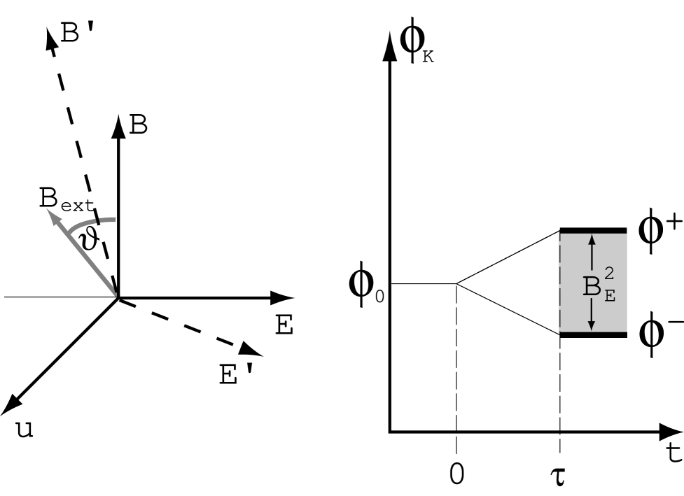
FIG. 3.: Intrinsic fields of the particle and external magnetic field. The external field $B_{ext}$ is perpendicular to the direction of motion and in an angle $\vartheta$ with the particle’s intrinsic field $B$ (left). The kinetic energy density is changed to two separate levels $\phi^{+}$ and $\phi^{-}$. The difference between these two levels is equal to $B_{E}^{2}$. Note that the change of the energy occurs continuously within the interval $t\in[0,\tau]$ (right).

The change of the phase velocity leads to a phase shift of the beam component in the magnetic field compared to the phase of the reference beam. This shift is linear with the amplitude of the magnetic field. Summing up the results in homogeneous fields we can say that the treatment allows to recover all features of the result in quantum mechanics (two discrete and symmetric solutions for the kinetic energy and the phase velocity, phase shifts linear with the amplitude of the field), while it gives a fully deterministic and local treatment of the process. An application of the result to atomic physics, which we will give in a follow up publication, accounts for the main features of the normal Zeeman effect in atomic physics.

B Inhomogeneous fields: Stern-Gerlach experiments

In inhomogeneous fields the magnetic intensity and amplitude depends on the location ${\bf B}_{ext}={\bf B}_{ext}({\bf r})$. In particular, in the setup of Stern-Gerlach experiments [5], the magnetic field changes along the $z$-axis of the coordinate system:

$${\bf B}_{ext}({\bf r})\equiv{\bf B}_{ext}(z)\qquad\frac{\partial{\bf B}_{ext}(z)}{\partial z}\neq 0$$ (33)

We assume, for the following, that the magnetic field is switched on in $t\in[0,\tau]$, and that $\tau$ is independent of $z$. Then the kinetic energy density $\phi_{K}(\tau,z)$ equals:

$$\delta\phi_{K}(\tau,z)=\frac{1}{2}B_{ext}^{2}(z)$$ (34)

Taking the gradient of the energy gives the local change of energy and thus a Newtonian potential and a Newtonian force acting on the particle:

$$F_{z}=-\frac{\partial\delta\phi_{K}(z,\tau)}{\partial z}=-B_{ext}(z)\frac{\partial B_{ext}(z)}{\partial z}$$ (35)

Accounting for real and imaginary components of the external field $B_{ext}$ gives, as in the homogeneous field, two symmetric solutions. These solutions describe the force perpendicular to the particle’s path of motion:

$$F_{z}=\pm B_{E}(z)\frac{\partial B_{E}}{\partial z}$$ (36)

The trajectory of the particle will be affected by this force. Writing it as an acceleration acting on the particle’s density of mass $\rho_{0}$, we get finally:

$$\frac{du_{z}}{dt}=\pm\frac{B_{E}(z)}{\rho_{0}}\frac{\partial B_{E}(z)}{\partial z}$$ (37)

This reflects the standard result in Stern-Gerlach experiments: two symmetric solutions on either side of the zero point and in the direction of the field gradient.

C The natural system of units

For reasons of consistency one has to use natural units in this calculation. In this system of physical units the interface between electrodynamics and mechanics is described by $\hbar$, Planck’s constant [15]. The fields and energies, in natural units, take the following form (terms of $4\pi$ generally omitted in the one-dimensional case):

$$\phi = \frac{\hbar}{2}\left({\bf E}^{2}+c^{2}{\bf B}^{2}\right)$$ (38)

$$\left[\phi\right] = \left[Jm^{-3}\right]$$ (39)

$$\left[{\bf E}\right] = \left[Nm^{-3}\right]$$ (40)

$$\left[{\bf B}\right] = \left[Nm^{-3}sm^{-1}\right]$$ (41)

$$\left[\hbar\right] = 1.054\times 10^{-34}\left[m^{4}N^{-1}\right]$$ (42)

Then the results for homogeneous fields, and including $\hbar$, are the following:

$$\delta\phi_{K}^{\pm}(\tau) = \mp\frac{\hbar}{2}\,c^{2}B_{E}^{2}$$ (43)

$$\delta u^{\pm}(\tau) \propto \pm\frac{\hbar}{2}\,B_{E}$$ (44)

The two symmetric solutions in the inhomogeneous field are:

$$F_{z}^{\pm} = \pm\frac{\hbar}{2}\,\frac{\partial}{\partial z}\,c^{2}B_{E}^{2}$$ (45)

$$\frac{du_{z}(\tau)}{dt} = \pm\frac{\hbar}{2}\,\frac{\partial}{\rho_{0}\partial z}\,c^{2}B_{E}^{2}$$ (46)

The main difference between a charged particle and a neutral one in a magnetic field is the change of the motion due to Lorentz forces. A neutral atom, even though its electrons may experience these forces, is not affected by Lorentz forces. In first approximation one may therefore treat the atom as a neutral particle in magnetic fields. Considering, that electron mass will experience the same shift of fields and consequently the same changes of kinetic energy in a dynamic model of atoms [23, 15], the results derived must also apply for motion of a neutral atom in an inhomogeneous magnetic field. The observation of two symmetric trajectories was, of course, one of the first experimental results obtained by Stern and Gerlach [5].

D Magnetic interactions: the general picture

In general, as outlined in the foundations of microdynamics [14], one has to account for two components of particle energy: the energy contained in its electromagnetic fields, and its kinetic energy. Both components together yield the total energy density of a particle, which is a constant of motion:

$$\phi_{T}=\rho_{T}u^{2}=constant$$ (47)

The amplitude is commonly irrelevant, since it does not show up in the differential equations describing the system. But the distribution between kinetic and field components of energy, depending, for a given moment or location, on the phase of the wave, must be included in the picture. A standard way to achieve this, is using imaginary components. From the viewpont of electromagnetic fields we may add imaginary contributions to the - real valued - magnetic fields. From the viewpoint of kinetic energy the field components are best described by imaginary components to a particles wavefunction, where $\psi^{2}=\rho$, the particle’s density of mass. We therefore get, in general, for $\phi({\bf r},t)$ and $\rho({\bf r},t)$ the following relations:

$$\phi({\bf r},t) = \frac{\hbar}{2}\left[c\cdot{\bf B}({\bf r},t)\right]^{2}\qquad{\bf B}({\bf r},t)=(B_{r}+iB_{i}){\bf e}_{B}$$ (48)

$$\rho({\bf r},t) = \psi^{2}({\bf r},t)\qquad\psi({\bf r},t)=\psi_{R}+i\psi_{i}$$ (49)

The relation between the scalar fields $\phi$ and $\rho$ (see Eq. (9)) is then multivalued, it depends on the distribution between the real and the imaginary components. Physically speaking, it depends on the exact moment, when the particle begins interacting with the external field. Since the intrinsic fields of the particle are periodic, it depends on the phase of the fields. And as there is, in addition, a continuous shift of energy from the field components to the kinetic components of a particle’s energy and vice versa, the real and complex components of the wavefunction are in general not zero. The same is true for the scalar field. The cases we have outlined so far are only the degenerate ones with:

$$(I) \qquad B_{r}\neq 0\quad B_{i}=0\qquad\psi_{r}\neq 0\quad\psi_{i}=0$$ (50)

$$(II) \qquad B_{r}\neq 0\quad B_{i}=0\qquad\psi_{r}=0\quad\psi_{i}\neq 0$$ (51)

$$(III) \qquad B_{r}=0\quad B_{i}\neq 0\qquad\psi_{r}\neq 0\quad\psi_{i}=0$$ (52)

$$(IV) \qquad B_{r}=0\quad B_{i}\neq 0\qquad\psi_{r}=0\quad\psi_{i}\neq 0$$ (53)

A further degeneracy arises from the equivalence of case I, IV and case II, III. For an arbitrary relation between intrinsic particle components and external field components the real and imaginary parts of the fields comply with:

$$\frac{\hbar}{2}\,\triangle\left(B_{r}+iB_{i}\right)^{2}+\frac{\partial^{2}}{c^{2}\partial t^{2}}\left(\psi_{r}+i\psi_{i}\right)^{2}=0$$ (54)

All components, in this general case, are non-trivial solutions of the differential equation. Note that this is no longer a linear equation. The non linearity thus enters the framework of microphysics at the energy transfer from field components to kinetic components and vice versa. Or, generally speaking, at the transition from electrodynamics to quantum mechanics. While both theories, in themselves, are linear, the general theory, including all interactions, is not. In the long term we expect this feature of microdynamics to provide the most interesting deviations from the purely linear frameworks employed in standard theory. Writing the relation as a system of two nonlinear equations for real and imaginary components, we get:

$$\frac{\hbar}{2}\,\triangle\left(B_{r}^{2}-B_{i}^{2}\right)+\frac{\partial^{2}}{c^{2}\partial t^{2}}\left(\psi_{r}^{2}-\psi_{i}^{2}\right)=0$$ (55)

$$\frac{\hbar}{2}\,\triangle B_{r}B_{i}+\frac{\partial^{2}}{c^{2}\partial t^{2}}\psi_{r}\psi_{i}=0$$ (56)

It is now easy to see that the degenerate solutions of (50) are equivalent to the trivial solutions of Eq. (56).

Note that the results apply to massive particles. In quantum mechanics massive particles are fermions. In addition, the theoretical framework is non-relativistic, so it can be applied with confidence only to the low energy limit of particle motion. Whether a similar picture is suitable for bosons, cannot be decided at present. Especially, since the archetypical bosons, photons, are relativistic and it has been shown, within the current framework, that interactions in this range are changed due to spacetime transformations in moving coordinate frames [24].

IV Measurements and statistics

An common feature of all results, for homogeneous as well as inhomogeneous fields, is that only two numerical values are generally decisive for the outcome of a measurement: the magnetic field (or its gradiant) and the Planck constant, or rather $\hbar/2$. Even though material parameters of atoms will enter an evaluation of (45), the functional form remains the same: a constant multiplied by a gradient and some material parameter. And the constant is incidentally equal to the spin of a particle.

In quantum mechanics it is generally thought that the particle is in a state ”spin-up” or ”spin-down” or a superposition of both. A measurement with a Stern-Gerlach device in an arbitrary direction $z$ leaves the particle in one of either states, but now with reference to the direction $z$. This is the notorious collapse of the wavefunction. The statistics on quantum mechanics, even though their change in a measurement is still not explained consistently, arise from the qualities of the particles themselves.

In the present picture the statistics arise from the interaction with the magnetic field. In this sense it is correct to say that the particle, before the measurement, does not have a defined property. But does it have defined properties after the measurement? Only, if we concede that the changes due to the applied fields are permanent. This would require some kind of resistivity, which we have not introduced.

In principle, this feature can be added to the model by some kind of internal friction. However, at this point we thought it sufficient to introduce the theory without it, because it is not clear, whether the feature is at all needed. Only experiments are suitable, in our view, to decide on this point. We shall describe a possible experiment to this end further down.

Note, in this respect, that a Stern-Gerlach device is not the same as an optical polarizer. Even though the two measurements are treated similarly in quantum mechanics, the polarization measurement leaves the photon in some final state. A repetition of the measurement can only confirm this state. The state of the particle or an atom after an interaction with a magnetic field depends on the changes made by the measurement. In the current picture, these changes are reversibel: when the atom leaves the field, its properties are the same as before. In this case a repetition of the same deflection - which is what an idealization in quantum mechanics predicts in every case - depends on an identical interaction process also for the second measurement. In case this is not observed, two explanations seem possible: (i) Decoherence effects between the atom and the experimental devices lead to a mixture of different spin states (this would be the explanation in quantum mechanics), or (ii) the atomic electron is not polarized at all (this is the theoretical prediction in the current model, not including irreversible effects). It seems interesting to check these possibilities by high-precision measurements.

Theoretically speaking, the change of an undefined combination of particle states before the measurement to a defined particle state after the measurement is not a desirable feature of such an experiment. Because, as already mentioned, it raises the problem of the collapse of the wavefunction. Based on the treatment given in this paper it seems that the problem could find its solution in the least expected way: there is, maybe, no collapse for this sort of measurement. All the more reason for a careful revision of Stern-Gerlach experiments.

The suggested theory can be checked experimentally by standard Stern-Gerlach experiments. There are two distinct differences between this model and the conventional model in quantum mechanics.

• The first one concerns the forces of deflection in a single Stern-Gerlach measurement. In quantum mechanics this force depends only on the gradient of the field:

  $$F_{QM}\propto\frac{\partial B_{z}}{\partial z}$$ (57)

  In the current model the force depends on the gradient of the field and the amplitude of the field:

  $$F_{MD}\propto B_{z}\frac{\partial B_{z}}{\partial z}$$ (58)

  The difference should be measurable in any high-precision measurement, since it concerns not so much absolute values but the dependency on the changes of magnetic fields.

• The second difference applies to multiple Stern-Gerlach experiments. Provided the process really is reversible, the prediction differs significantly between quantum mechanics and this model. This effect is far less significant, because decoherence will in practice destroy the distinction between the states. But even then the difference should be observable.

V Spin in quantum mechanics

In quantum mechanics the magnetic moment of a particle, and hence its spin, is defined to comply with measurements. The measurements yield two possible results, independent of any orientation of the magnet [5]. The experimental results therefore exclude a single valued function for the magnetic moment of a particle. Thus the classical picture, with its vector relation:

$$W=-{\bf\mu}{\bf B}\qquad{\bf\mu},{\bf B}\in R^{3}$$ (59)

is unsuitable to describe events at this level. We found in the preceding sections that even the two-valuedness could be a simplification. It takes only two single points of the whole parameter space into account. This parameter space is defined by the phase of the particle’s intrinsic and the external magnetic field.

A Conservation laws and phase relations

Spin cannot be interpreted as a rotation of an extended object around a defined but hidden direction in space. Even though such a correspondence can be carried out to some extent (see for example Bohm and Hiley [25]), it is ultimately insufficient. The reason is twofold: (i) The angular velocity of a particle’s surface exceeds the velocity of light. (ii) The degree of freedom for the N-particle wavefunction of $2^{2N+1}$ is much higher than the physically relevant parameters of the system (proportional to $N$).

In our view, these aspects just point to different consequences of the same basic assumption: the motion of independent entities, with defined properties and existing independently of each other. From the viewpoint of quantum mechanics the total wavefunction of a system is a Slater determinant of single particle wavefunctions. This combination is commonly interpreted as a statistical feature of quantum systems. We interpret it, slightly different, as the simplest combination, which retains linearity throughout the system. It is therefore connected to the field properties of particles, and not particularly to statistics. The interpretation bears on a shortcoming of conservation laws in classical mechanics. It explains, why these entities (single particles) cannot be treated independently from each other in a field theoretical context. In this sense it explains, from a realistic and strictly physical (as opposed to mathematical) point of view, why quantum mechanics cannot be seen as a mechanical theory in any classical sense.

In general, conservation laws have two objectives: The first is to define the standard of a formalization, or the zero point of a description. This essentially Newtonian aspect (it is but a different form of his first principle) considerably facilitates the description of a system, because only changes of energy, momentum etc. need to be described. The second objective is the identification of different objects with the same general case. Every object with the same properties (energy, momentum etc.) can be described with the same numbers, it is the same object. But while this holds generally in classical mechanics, it is not true in classical electrodynamics. Because in this case the phase of the field is generally relevant. So that even in the case when the field is finite, the phase of intrinsic electromagnetic fields cannot remain unconsidered. In a nutshell: an electron or photon with the same energy, linear momentum, and polarization as another electron or photon can not necessarily be described in the same way. Not, if the phase along its path of propagation is different. In this sense the identification in field physics is more constrained than it is in mechanics. The additional constraint is the phase relation. For this very reason the assumption in quantum mechanics, that two objects (= states), which differ only by a phase $e^{i\varphi}$, are identical, is not generally valid. It makes a difference, if the phase of a single particle of a pair is changed by $e^{i\varphi}$. Because in this case correlation measurements are altered [16]. Therefore the degeneracy with respect to the phase of a particle’s wavefunction is not a general feature [26]. And since this effect can be measured - and is measured with high precision in quantum optics - the current framework of quantum mechanics, where the phase is seen as arbitrary [27], needs to be modified.

B Spin and interactions in quantum mechanics

It is standard procedure to refer the mathematical representation of spin via Pauli matrices to a necessary modification of the angular momentum [28]. The modification is due to the experimental result of only two values for the magnetic interactions. It leads to a modified Schrödinger equation, the Pauli equation:

$$\left[\frac{1}{2m}\left(\hat{\bf p}-e{\bf A}\right)^{2}+\mu_{B}\hat{\bf\sigma}{\bf B}\right]\Psi=i\hbar\frac{\partial}{\partial t}\Psi$$ (60)

where $\mu_{B}$ is the Bohr magneton and $\Psi=(\psi_{1},\psi_{2})$ is a two-spinor. The interaction in magnetic fields is now described by the term $\hat{\bf\sigma}{\bf B}$.

This description of spin via Pauli matrices is not limited to magnetic properties. It can be used quite generally to describe two-level systems. In nuclear physics, for example, it is employed to describe the state ”proton” and the state ”neutron” of a nucleon. Therefore it appears to be generally applicable. But in this case it cannot carry enough physical significance, to make it analog to an angular momentum. And then we may ask, whether it tells us anything more about a system than precisely this: whatever you measure about spin, you always get exactly two symmetric results. The value of these results, for a single particle, being defined to fit the measurements in atomic physics. And since all of these measurements are logically connected via the Pauli (Schrödinger) equation, the definition is unique. The results we have presented suggest that spin is only mathematically, but not physically meaningful. It was proved that the interpretation of spin as an angular momentum is wrong. And it was shown, how two discrete solutions arise in every interaction of a particle with a magnetic field. These discrete solutions are commonly interpreted as ”spin states” of fermions.

We are now in the position to understand, why spin, in quantum mechanics, seems such a peculiar concept. In particular we can now try to answer the questions, why it must be described by Pauli matrices; why these spin-operators are linear and essentially abstract; and why they must lead to two discrete solutions. Beginning with the first question, we can say that:

• Since magnetic interactions affect the intrinsic features of a particle, and since they lead, in a dynamic picture, to two symmetric solutions, spin must be a non-unique and two-valued function.

The rotational features of spin, most notably its $4\pi$ symmetry, also derive from the two-valuedness. The Pauli matrices are a simple way to secure this property.

• Because interactions are generally invariant to rotations of field vectors in the system of a particle, spin cannot be described as a two-valued vector in real-space.

The eigenvectors of spin must therefore be abstract (not real-space) entities. Again, the spin matrices and the eigenspace related to it just describe the simplest mathematical structures operating in such a way. However, the physical process underneath these mathematical entities is a completely different one. It is the continuous and dynamic change of the field properties of particles, when they enter a magnetic field, which is described in this abstract manner.

Also this problem, why quantum mechanics cannot describe the physics behind its mathematical concepts, comes from the mechanical perspective. Because it is assumed in quantum mechanics that we can give an integral description of the process by simply multiplying a quality of the external field (${\bf B}$) with a quality of the particle ($\hat{\bf\sigma}\cdot\psi$). Ultimately the problem comes from the assumed analogy with the magnetic moment. In microdynamics no such problem exists. The fields remain perfectly defined during the whole interaction process. The dynamic picture thus gives a precise spacetime account of interactions. A feature, which is impossible to achieve in quantum mechanics. Not, because microphysics had any special properties to reckon with, but because quantum mechanics uses unsuitable (mechanical) analogies.

• The two symmetric results are the simplest degenerate cases for magnetic interactions. They originate from the arbitrary phase of the particles intrinsic and the external fields. In particular from the existence of field components and kinetic components of energy density.

In the general case the interaction is expected to exhibit a greater variety of possible results. How this general case is to be formalized, and how interactions are to be calculated, remains to be described in future. The relevant message, at this point, is only the following:

Spin appears to be a simplification of particle properties. This simplification has its roots in the mechanical analogy. Field theoretical models, considered by the author to be generally superior, may change the way we describe microphysical systems quite substantially. In addition, the whole model, if verified, proves once more that quantum mechanics has achieved only the fundamentals of the transition from macrophysics to microphysics. In the long term it is thus more appropriate to build upon a suitably modified field theoretical model. And the theory of microdynamics seems to provide just such a model.

VI Conclusion

In this paper we have given a precise spacetime account of magnetic interactions. The model is based on the intrinsic properties of particles, generally employed in microdynamics. We could show that homogeneous and inhomogeneous magnetic fields in the simplest degenerate cases allow for two symmetric solutions. This result is verified in experiments. We have analyzed the difficulties in quantum mechanics to describe these measurements in a continuous model, and we found that they arise from unsuitable mechanical analogies, in particular the analogy of angular momentum. Finally, we pointed out possible experiments to check the model derived against the standard model in quantum mechanics.

REFERENCES

- [1] R. Mirman, Group theoretical Foundation of Quantum Mechanics, Nova Science, Huntington NY (1995)
- [2] U. Fano and A.R.P. Rau, Symmetries in Quantum Physics, Academic Press, San Diego CA (1996)
- [3] N. Bohr, Phys. Rev. 48, 696 (1935)
- [4] J.D. Jackson, Classical Electrodynamics, 3rd edition, Wiley & Sons, New York (1999) pp. 174 - 190
- [5] W. Gerlach and O. Stern, Ann. Physik 74, 673 (1924); the standard reference on these experiments is by N.F. Ramsey, Molecular Beams, Oxford University Press, Oxford UK (1956)
- [6] G.E. Uhlenbeck and S.A. Goudsmit, Naturwiss. 13, 953 (1925);
- [7] G.E. Uhlenbeck and S.A. Goudsmit, Nature 117, 264 (1925)
- [8] W. Pauli, Phys. Rev. 58, 716 (1940)
- [9] The Theory of the Electron, J. Keller and Z. Oziewicz (ed.) UNAM, Mexico (1997)
- [10] N. Bohr in A. Einstein: Philosopher-Scientist, P.A. Schilpp (ed.), Harper and Row, New York (1959)
- [11] B. d’Espagnat, Conceptual Foundations of Quantum Mechanics, Addison Wesley, New York (1989)
- [12] N.D. Mermin, Phys. Today 38, No. 4, 38 (1985)
- [13] For a non-technical overview of the theory see the following website: www.cmmp.ucl.ac.uk/wah/md.html
- [14] W.A. Hofer, Physica A 256, 178-196 (1998)
- [15] W.A. Hofer, Evidence for a dynamic origin of charge, quant-ph/0001012
- [16] W.A. Hofer, Information transfer via the phase: A local model of Einstein-Podolsky-Rosen experiments, quant-ph/0006005
- [17] P.R. Holland, The Quantum Theory of Motion, Cambridge University Press, Cambridge (1993)
- [18] W.A. Hofer, Measurements in quantum physics: A new theory of measurements in terms of statistical ensembles, Proceedings of the VIth Wigner Symposium, August 16-22 1999, Istanbul
- [19] A. Zeilinger, R. Gaehler, C.G. Shull and W. Teimer Symposion on Neutron Scattering, Argonne National Lab. (Am. Inst. Phys., 1981)
- [20] H. Rauch, Neutron interferometric tests of quantum mechanics, in F. Selleri (ed.) Wave-article duality, Plenum Press, New York (1992)
- [21] E. Merzbacher, Quantum Mechanics, Wiley & Sons, New York (1998)
- [22] K. Gottfried and V. Weisskopf according to M.H. MacGregor, The Enigmatic Electron, Kluwer, Dordrecht (1992) p.6
- [23] W.A. Hofer, A dynamic model of atoms: structure, internal interactions and photon emissions of hydrogen, quant-ph/9801044
- [24] W.A. Hofer, A realist view of the electron: recent advances and unsolved problems, in Contemporary Fundamental Physics, V.A. Dvoeglazov (ed.), Nova Science, Huntington NY (2000)
- [25] D. Bohm and B.J. Hiley, The Undivided Universe, Routledge, London (1993) pp. 204 - 214
- [26] In the meantime, Charim Anastopoulos seems to have reached a similar conclusion, see Quantum theory without Hilbert spaces, quant-ph/0008126
- [27] E.P. Wigner, Group Theory and its Applications to the Quantum Mechanics of Atomic Spectra, New York, Academic Press (1959) p. 233
- [28] W. Greiner, Quantum theory, Springer Verlag Berlin (1994) pp. 299 - 315