[

Experiments towards Falsification of Noncontextual Hidden Variable Theories

Abstract

We present two experiments testing the hypothesis of noncontextual hidden variables (NCHV’s). The first one is based on observation of two-photon pseudo-Greenberger-Horne-Zeilinger correlations, with two of the originally three particles mimicked by the polarization degree of freedom and the spatial degree of freedom of a single photon. The second one, a single-photon experiment, utilizes the same trick to emulate two particle correlations, and is an “event ready” test of a Bell-like inequality, derived from the noncontextuality assumption. Modulo fair sampling, the data falsify NCHV’s.

]

The statistical nature of quantum predictions has frequently initiated efforts to expand the quantum mechanical description. The so-called hidden variable concepts try to cure the quantum indeterminism by ascribing values to the properties of a system which are defined already prior to the measurement. The question arises whether such expansion of the theory is justified.

noncontextual hidden variable (NCHV) theories assume that the predetermined result of a particular measurement does not depend on what other observable is simultaneously measured (see e.g. [1]). Such cryptodeterminism was ruled out by the Bell-Kochen-Specker (BKS) theorem [2], which, as a mathematical theorem, does not need experimental confirmation – and neither suggests one. Yet, quite recently, doubts arose about the usefullness of the BKS theorem due to the impossibility of experimentally testing the yes/no contradiction of the BKS theorem in real world, where one is always confined to finite measurement times and precision[3]. NCHV theories form a subset of local realistic hidden variable (LHV) theories, which rely on the more plausible assumption that the predetermined result of a particular measurement does not depend on what other observable is simultaneously measured in a spatially separated region. Bell’s theorem [4] gives a clear prescription for a statistical test of LHV theories. However, almost all experiments testing LHV theories do not enforce spacelike separation of measurements, and all are plagued with the low detection efficiency, thus falling short of definitely invalidating LHV theories [5].

We report two experiments testing the validity of NCHV theories. The experiments are much simpler than equivalent Bell tests (with no strict imposition of locality), and much less sensitive to experimental imperfections. This includes lower threshold interference visibility and consequently also less demanding threshold for detection efficiencies. The possible adaptation to other quantum systems paves the way to a loophole-free test of the particular class of noncontextual hidden variable theories. Formally, the experiments are employing the fact, that measurements on distinct tensor product factors of Hilbert space commute and can therefore form varying contexts for one another. In the analysis of these experiments we obtain, for a specific state [6], verifiable, statistical conditions for the measurement results. In the first experiment the three particle GHZ theorem [7, 8], by using its version for NCHV theories [9], is reduced to one with only two particles. In the second one an “event-ready” test of a Bell-like inequality for only one particle allows to validate NCHV theories [10].

If a NCHV theory attempts to reproduce quantum predictions it must fulfill some basic prerequisites. First, the predetermined value $a_{i}$, which is revealed when measuring the property $\overline{A}$ for a given individual system $i$, i.e. a single run of the experiment, must be equal to one of the eigenvalues of the quantum mechanical observable $\hat{A}$ identified with this property. Further, in quantum mechanics, any real function $f(\hat{A},\hat{B})$ of commuting, and thus commeasurable observables $\hat{A},$ $\hat{B}$ is also an observable, and the eigenvalues of such a function observable are given by $f({A},{B}),$ where ${A},$ ${B}$ are eigenvalues of the respective operators. In a NCHV theory, this rule of functional dependence must also hold for the preexisting values; i.e., $f(\overline{A},\overline{B})_{i}=f(a_{i},b_{i})$. We will see, that there are input states to function observables for which NCHV theories and quantum mechanics give conflicting predictions, and which thus enable experimental tests.

The photon’s momentum (and thus its propagation direction) commutes, and thus is commeasurable with the photon’s polarization. We utilize this fact to define the observables in our experimental test of NCHV theories. The first observable $\hat{A}(\phi_{A})$ is the direction of photon propagation behind the (nonpolarizing) beam splitter BS (Fig. 1) and has eigenvalue $A=+1$, if the photon is found in the upper exit, and $A=-1$, if in the lower one. The relative phase $\phi_{A}$ between the two input paths is a free parameter of this observable and determines the actual eigenstates.

The second observable, $\hat{B}(\phi_{B})$, is the polarization of the same photon. Its result $B=\pm 1$ is determined operationally by the exit port of a polarizing beam splitter (PBS), where the photon is detected. The actual polarizations distinguished by the PBS are set by a birefringent phase $\phi_{B}$. A third observable $\hat{C}(\phi_{C})$ acting on another photon is identical in its nature to $\hat{B}(\phi_{B})$.

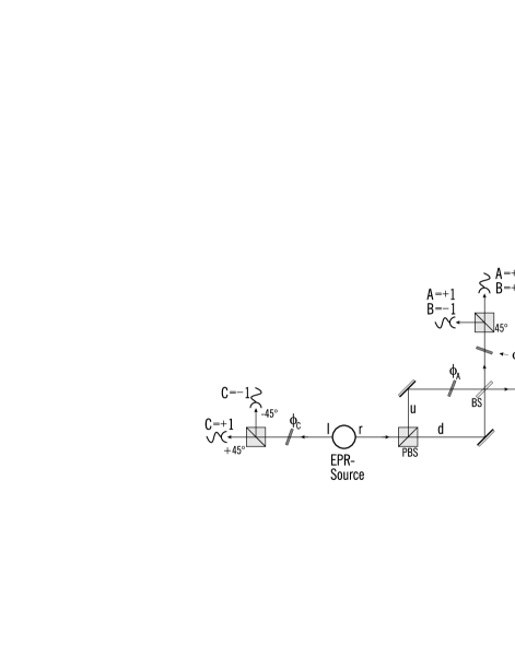
FIG. 1.: Experimental set up to test noncontextual hidden variable (NCHV) theories by determining correlations between the results of commeasurable properties. These properties are the propagation direction of a photon behind a beam splitter (BS), $\overline{A}$, and the polarization of the photon, $\overline{B}$, as determined by a polarizing beam splitter (PBS) oriented at 45^∘ and the birefringent phases $\phi_{B}$. The third observed property is the polarization of a second photon, $\overline{C}$. Depending on the relative phase $\phi_{A}$ between the inputs to the beam splitter and on the birefringent phases $\phi_{B}$ and $\phi_{C}$, for certain input states the results exhibit correlations which cannot be described by NCHV theories. (For details of the actual layout see text.)

Fig. 1 shows the experimental setup. Two polarization entangled photons emerge from the source in the state

$$\left|\,\psi_{initial}\right\rangle=\frac{1}{\sqrt{2}}\left(\left|\,H\right\rangle_{2}\left|\,V\right\rangle_{1}+\left|\,V\right\rangle_{2}\left|\,H\right\rangle_{1}\right)\left|\,l\right\rangle_{2}\left|\,r\right\rangle_{1},$$ (1)

where $H$ and $V$ denote the linear polarizations, $l$ and $r$ direction of propagation, and the subscripts $1$ and $2$ enumerate the photons. After the polarizing beamsplitter (PBS), which is oriented such that it transmits H polarization and reflects V polarization, the state changes into

$$\left|\,\psi\right\rangle=\frac{1}{\sqrt{2}}\left(\left|\,H\right\rangle_{2}\left|\,V\right\rangle_{1}\left|\,u\right\rangle_{1}+\left|\,V\right\rangle_{2}\left|\,H\right\rangle_{1}\left|\,d\right\rangle_{1}\right)\left|\,l\right\rangle_{2},$$ (2)

where $u$ and $d$ denote the two exit beams of the PBS. The factor in the bracket has the formal structure of the GHZ state. The third particle is emulated by an additional degree of freedom of particle $1$, which now is also entangled with the polarization of particle $2$.

The beamsplitter (BS) together with the phase shifter in front of it transforms the input modes $|u\rangle$ and $|d\rangle$ into two output modes, $\left|\,\pm 1,\phi_{A}\right\rangle=\frac{1}{\sqrt{2}}(i\left|\,d\right\rangle_{1}\pm e^{i\phi_{A}}\left|\,u\right\rangle_{1})$. If detection of photon 1 happens behind the upper exit of the BS we shall say that the eigenvalue $+1$ of the dichotomic observable, $\hat{A}(\phi_{A})=\left|\,+1,\phi_{A}\right\rangle_{11}\langle+1,\phi_{A}|-\left|\,-1,\phi_{A}\right\rangle_{11}\langle-1,\phi_{A}|$, was obtained, otherwise the eigenvalue is $-1$. Detection behind one of the final PBS performs, together with the birefringent phase plate $\phi_{B}$ (with fast axis along V), a projection onto the states $\left|\,\pm 1,\phi_{B}\right\rangle=\frac{1}{\sqrt{2}}(\left|\,H\right\rangle_{1}\pm e^{i\phi_{B}}\left|\,V\right\rangle_{1})$. Photon 2 is analyzed by the polarization observable $\hat{C}(\phi_{C})$. For convenience of formal description, $\phi_{C}$ is realized by a birefringent plate with fast axis along H, i.e., $\left|\,\pm 1,\phi_{C}\right\rangle=\frac{1}{\sqrt{2}}(\left|\,V\right\rangle_{2}\pm e^{i\phi_{C}}\left|\,H\right\rangle_{2})$. The formal definition of $\hat{B}(\phi_{B})$ and $\hat{C}(\phi_{C})$ follows the pattern of $\hat{A}(\phi_{A})$.

The quantum prediction for a photon prepared in state (2) to be detected in one of the detectors which are assigned values $A=\pm 1$ and $B=\pm 1$, and simultaneously the other photon to be detected in one of the exits $C=\pm 1$, is given by

$$P(A,B,C|\phi_{A},\phi_{B},\phi_{C})$$ (3)

$$=|(_{1}\langle A,\phi_{A}|_{1}\langle B,\phi_{B}|_{2}\langle C,\phi_{C}|)|\psi\rangle|^{2}$$ (4)

$$=\frac{1}{8}\left(1+ABC\sin{(\phi_{A}+\phi_{B}+\phi_{C})}\right).$$ (5)

The correlation function for the mean value of the product of the three commeasurable observables monitored in the first experiment is given by

$$E(\phi_{A},\phi_{B},\phi_{C})$$ (6)

$$=\langle\psi|\hat{A}(\phi_{A})\hat{B}(\phi_{B})\hat{C}(\phi_{C})\left|\,\psi\right\rangle=\sin{(\phi_{A}+\phi_{B}+\phi_{C})}.$$ (7)

In the second experiment, the registration of photon 2 serves as trigger for the event-ready operation of the experiment on photon 1. After the trigger event in the $45^{\circ}$ exit of the left PBS, photon 1 propagates in the state $\frac{1}{\sqrt{2}}(\left|\,H\right\rangle_{1}+\left|\,V\right\rangle_{1})\left|\,l\right\rangle_{1}$, which changes behind the right PBS into $\left|\,\psi^{\prime}\right\rangle_{1}=\frac{1}{\sqrt{2}}(\left|\,V\right\rangle_{1}\left|\,b\right\rangle_{1}+\left|\,H\right\rangle_{1}\left|\,a\right\rangle_{1})$. The correlation function for the product of the observables $\hat{A}(\phi_{A})$ and $\hat{B}(\phi_{B})$ reads

$${\cal E}(\phi_{A},\phi_{B})=\langle\psi^{\prime}|\hat{A}(\phi_{A})\hat{B}(\phi_{B})\left|\,\psi^{\prime}\right\rangle$$ (8)

$$=\sin{(\phi_{A}+\phi_{B})}.$$ (9)

Next, let us discuss the two experiments in terms of NCHV’s. For every emitted photon pair the commuting observables now must have preexisting values ${a}(\phi_{A})_{i}$, ${b}(\phi_{B})_{i}$, and ${c}(\phi_{C})_{i}$, which are equal to $+1$ or $-1$. Context independence here means that each of the values solely depends on the associated phase, but not on the other two phase settings. Therefore the correlation function must have the form:

$$E_{NCHV}(\phi_{A},\phi_{B},\phi_{C})=\frac{1}{N}\sum_{i=1}^{N}{a}(\phi_{A})_{i}{b}(\phi_{B})_{i}{c}(\phi_{C})_{i},$$ (10)

where $N$ is the (large) number of runs of the experiment.

Now, quantum mechanics predicts that the correlation functions $E(0,0,\pi/2)$, $E(0,\pi/2,0)$, and $E(\pi/2,0,0)$ are all equal to $1$. To reproduce such results the products of the preexisting values $a(0)_{i}b(0)_{i}c(\pi/2)_{i}$, $a(0)_{i}b(\pi/2)_{i}c(0)_{i}$, and $a(\pi/2)_{i}b(0)_{i}c(0)_{i}$ must therefore be all equal to $1$ in every single run of the experiment.

From these three observations one obtains the NCHV prediction for yet another set of phases. After multiplying the above three products and using the fact that the square of any of the preexisting values is one, it follows that the product $a(\pi/2)_{i}b(\pi/2)_{i}c(\pi/2)_{i}$ is always equal to +1. However, the resulting prediction, $E_{NCHV}(\pi/2,\pi/2,\pi/2)=1$, is in absolute contradiction to the quantum mechanical prediction, for which $E(\pi/2,\pi/2,\pi/2)=-1$.

In the second experiment, after the trigger detection of photon 2, only observables $\hat{A}(\phi_{A})$ and $\hat{B}(\phi_{B})$ need to be measured on the right side of the setup. For the preexisting context independent values $a(\phi_{A})_{k}$ and $b(\phi_{B})_{k}$ the Bell-type correlation function can be defined by

$${\cal E}_{NCHV}(\phi_{A},\phi_{B})=\frac{1}{M}\sum_{k=1}^{M}{a}(\phi_{A})_{k}{b}(\phi_{B})_{k},$$ (11)

where $k$ numbers the trigger events, and $M$ is their total number. Such correlation functions must satisfy the well known Bell-CHSH inequality

$$-2\leq{\cal E}_{NCHV}(\phi_{A},0)+{\cal E}_{NCHV}(\phi_{A},\pi/2)$$ (12)

$$+{\cal E}_{NCHV}(\phi_{A}^{\prime},\pi/2)-{\cal E}_{NCHV}(\phi_{A}^{\prime},0)\leq 2.$$ (13)

But quantum mechanic predicts values up to $2\sqrt{2}$.

For the experimental test of these contradicting predictions polarization entangled photon pairs are produced by type-II parametric down conversion and selected at a wavelength of 702nm. In the right arm a polarizing beam splitter was used to prepare the state of Eq. (2). Ideally, the polarizing beam splitter transmits horizontal polarization and reflects vertical polarization. In order to reduce residual H contributions in the reflected beam $u$ (for our PBS about 4%) and to obtain better state preparation, we placed another PBS (not shown in Fig. 1), rotated by 90^∘ in this beam. The paths are combined at a 50:50 beam splitter which is insensitive to polarization. The phase $\phi_{A}$ was locked to a dark fringe of a He:Ne interferometer adjacent to the down conversion light.

The observables $\hat{B}(\phi_{B})$ and $\hat{C}(\phi_{C})$ are measured behind Wollaston-type calcite prisms. The phases $\phi_{B}$ and $\phi_{C}$ are set with quartz plates, with the fast axis oriented vertically for $\phi_{B}$ and horizontally for $\phi_{C}$. The phases are determined by the birefringence of quartz and do not need any stabilization on the time scale of the experiment (about 50min).

Finally, after passing narrowband interference filters ($\Delta\lambda=5$ nm) the light was coupled to fiber pigtailed Silicon single photon avalanche detectors. Only four detectors were employed, i.e. the results $A=-1;B=-1$ and $A=-1;B=+1$ have not been registered directly.

The symmetries of the experiment, particularly between the outputs of the beam splitter BS, enable one to assume that the probability to observe $(A=+1;B=+1;C=+1)$ is equal to the probability of the result $(A=-1;B=-1;C=+1)$, and similarly for the other cases. Thus the correlation function $E_{obs}(\phi_{A},\phi_{B},\phi_{C})$ can be obtained from

$$E_{obs}(\phi_{A},\phi_{B},\phi_{C})=2\sum_{B,C}(BC)P(1,B,C|\phi_{A},\phi_{B},\phi_{C}).$$

Fig. 2 shows the correlation functions for different settings of the phases $\phi_{B},\phi_{C}$, when varying the phase $\phi_{A}$ [11]. For demonstrating a noncontextual GHZ-like contradiction one first has to establish the behaviour for the phase settings $(\pi/2,0,0)$, $(0,\pi/2,0)$, and $(0,0,\pi/2)$. From the raw data, i.e. not corrected for background, detector efficiencies etc., we obtain the following values for the correlation functions: $E_{obs}\left(0.46\pi,0,0\right)=0.885$, $E_{obs}\left(0.01\pi,\pi/2,0\right)=0.897$, and $E_{obs}\left(0.01\pi,0,\pi/2\right)=0.884$ [12]. With coincidence rates of about 500 s^-1 and a sampling time of 10 s (see Fig. 3), the error for these correlation values amounts to $\Delta E_{obs}=0.005$.

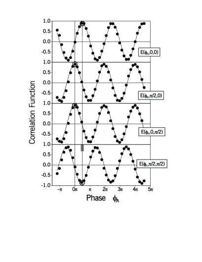
FIG. 2.: GHZ-like correlation functions obtained in the first experiment by varying phase $\phi_{A}$ for different settings of the birefringent phases $\phi_{B}$ and $\phi_{C}$. From the encircled data points of the first three correlation functions NCHV theories deduce a prediction for the fourth correlation function which has to lay within the shaded region. The contradiction with the data is evident.

From these measurements contradicting predictions are deduced within NCHV theories and quantum mechanics for the fourth measurement with the setting $(\pi/2,\pi/2,\pi/2)$. The results of Fig. 2 do not establish perfect correlations due to noise effects like imperfect components and mode quality of the down conversion fluorescence. Thus the contradiction between the two predictions cannot be observed directly. The problem of less than perfect correlations was already considered in the context of the GHZ paradox. Similarily, within a NCHV description, the correlation functions have to fulfill the following inequality [8, 13]:

$$2\geq E_{NCHV}(\phi_{A},\pi/2,\pi/2)-E_{NCHV}(\phi_{A},0,0)$$ (14)

$$-E_{NCHV}(\phi_{A}^{\prime},\pi/2,0)-E_{NCHV}(\phi_{A}^{\prime},0,\pi/2)\geq-2.$$ (15)

Thus, from the first three measurements NCHV theories predict for the fourth measurement a lower bound of $E_{NCHV}(0.46\pi,\pi/2,\pi/2)\geq 0.666\pm 0.008$, which is in strong disagreement with the observed value of $E_{obs}(0.46\pi,\pi/2,\pi/2)=-0.885\pm 0.005$.

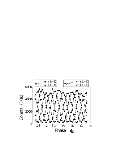
FIG. 3.: Conditioned count rate at detectors on the right side when varying the phase $\phi_{A}$ for two settings of $\phi_{B}$. The data at the angles indicated by arrows lead to a violation of a Bell-like inequality and thus again invalidate noncontextual hidden variable theories.

In the second experiment detection of photon 2 at detector $C=+1$ with $\phi_{C}$ set to zero serves as a trigger to prepare photon 1 with a polarization of 45^∘. One can pick up among the conditioned counts (Fig. 3) observing $\hat{A}(\phi_{A})$ and $\hat{B}(\phi_{B})$ the subset needed for calculating the correlation functions and obtains, directly from the raw data, $E_{obs}(-0.72\pi,0)=0.586\pm 0.008$, ${E}_{obs}(-0.72\pi,\pi/2)=0.705\pm 0.008$, $E_{obs}(0.75\pi,0)=-0.590\pm 0.008$, and $E_{obs}(0.75\pi,\pi/2)=0.714\pm 0.008$ (the data used are indicated by the arrows in Fig. 3). When evaluating the Bell-like inequality (13) with these values one obtains $2.595\pm 0.015>2$, i.e. we have again a gross violation of noncontextuality.

The experiments had the feature that the effective collection efficiency of photons was about 8%. Therefore, like in all known experiments testing the hidden variable theories, we have to invoke the fair sampling assumption.

The present approach leads to radical simplification of the experiments, which becomes possible when one concentrates on the problem of noncontextuality. Besides simpler setups and thus reduced noise contributions, these schemes require less efficient detection systems than standard Bell or GHZ experiments. For perfect visibilities the required detection efficiency reduces to $\sqrt{2}/2$. This value is still somewhat high for experiments with entangled photon pairs, but surely can be reached by other experimental techniques [14]. Not all hidden variable theories can be ruled out with this approach, but the large class of NCHV theories is now open to tests with single atoms or ions bringing loophole-free tests into reach.

We acknowledge discussions with Abner Shimony and Anton Zeilinger. This work was supported by the Austrian-Polish Program Quantum Information and Quantum Communication II 11/98b, by the UG Programs BW/5400-5-0264-9 and BW/5400-5-0032-0, by the Austrian FWF (Proj. Y48-PHY), and the German DFG (Proj. WE2451/1), the last stage by ESF Programme on Quantum information theory and quantum computation.

REFERENCES

- [1] N.D. Mermin, Phys. Rev. Lett. 65, 3373 (1990); N.D. Mermin, Rev. Mod. Phys. 65, 803 (1993).
- [2] J.S. Bell, Rev. Mod. Phys. 38, 447 (1966); S. Kochen and E. Specker, J. Math. Mech. 17 59 (1967).
- [3] D.A. Meyer, Phys. Rev. Lett. 83, 3751 (1999); A. Kent, Phys. Rev. Lett. 83, 3755 (1999).
- [4] J. S. Bell, Physics (Long Island City, N.Y.) 1, 195 (1965).
- [5] There are only two experiments which tried to enforce spacelike separation of the measurements: A. Aspect, J. Dalibard, and G. Roger, Phys. Rev. Lett. 49, 1804 (1982); G.Weihs, T. Jennewein, C. Simon, H. Weinfurter, and A. Zeilinger, Phys. Pev. Lett. 81, 5039 (1998). All others, in effect, are testing only NCHV-theories.
- [6] A. Peres (Phys. Lett. A 151, 107 (1990)), argues that the state independence the the original BKS paradox is only of an esthetic value. If there is no NCHV description for a specific state, neither there is one for the whole theory.
- [7] D.M. Greenberger, M.A. Horne, A. Zeilinger, in Bell’s Theorem, Quantum Theory, and Conceptions of the Universe, edited by Kafatos, M. (Kluwer Academics, Dordrecht, The Netherlands, 1989), p. 73;
- [8] N.D. Mermin, Phys. Rev. Lett. 65, 1838 (1990).
- [9] M. Żukowski, Phys. Lett. A 157, 198 (1991).
- [10] After the measurements had been done a similar idea (for neutrons) was presented the by S. Basu, S. Bandyopadhyay, G. Kar and D. Home, quant-ph9907030. For less operational proposals of tests of NCHV’s see: S. M. Roy and V. Singh, Phys. Rev. A 48, 3379 (1993); A. Cabello and G. Garcia-Alcaine, Phys. Rev. Lett. 80, 1797 (1998).
- [11] In order to regain the sinusoidal shape of the correlation function, for this figure only, the raw coincidence rates are corrected for different overall detection efficiencies.
- [12] Phases could be reproducibly set with an uncertainty of and .
- [13] L. Hardy, Phys. Lett. A 160, 1 (1991); N.D. Klyshko, Phys. Lett. A 172 399 (1993).
- [14] Q. A. Turchette, C. S. Wood, B. E. King, C. J. Myatt, D. Leibfried, W. M. Itano, C. Monroe, and D. J. Wineland, Phys. Rev. Lett. 81, 3631 (1998); E. Hagley, X. Ma tre, G. Nogues, C. Wunderlich, M. Brune, J. M. Raimond, and S. Haroche, Phys. Rev. Lett. 79, 1 (1997).