Natural Thermal and Magnetic Entanglement in 1D Heisenberg Model

Abstract

We investigate the entanglement between any two spins in a one dimensional Heisenberg chain as a function of temperature and the external magnetic field. We find that the entanglement in an antiferromagnetic chain can be increased by increasing the temperature or the external field. Increasing the field can also create entanglement between otherwise disentangled spins. This entanglement can be confirmed by testing Bell’s inequalities involving any two spins in the solid.

It is well known that distinct quantum systems can be correlated in a ”stronger than classical” manner [1, 2, 3]. This ”excess correlation”, called entanglement, has recently become an important resource in quantum information processing [4]. Like energy, it is quantifiable [5, 6, 7]. This motivates us to ask how much entanglement exists in a realistic system such as a solid (the likely final arena for quantum computing [8]) at a finite temperature. The 1D Heisenberg model [9, 10] is a simple but realistic [11] and extensively studied [12, 13, 14, 15] solid state system. We analyze the dependence of entanglement in this system on temperature and external field. We find that the entanglement between two spins in an antiferromagnetic solid can be increased by increasing the temperature or the external field. Increasing the field to a certain value can also create entanglement between otherwise disentangled spins. We show that the presence entanglement can be confirmed by observing the violation of Bell’s inequalities. However, on exceeding a critical value of the field, the entanglement vanishes at zero temperature and decays off at a finite temperature. In the ferromagnetic solid, on the other hand, entanglement is always absent. We compare the entanglement in these systems to the total correlations.

The entanglement of formation [5] is a computable entanglement measure for two spin-$\frac{1}{2}$ systems (qubits) [16]. We will use this measure to compute the entanglement between different spins in the 1D isotropic spin-$\frac{1}{2}$ Heisenberg model. This model describes a system of an arbitrary number of linearly arranged spins, each interacting only with its nearest neighbors. Recently, entanglement in linear arrays of qubits have attracted interest [18, 19, 20] and in Ref.[19] the entanglement in the ground state of a Heisenberg antiferromagnet has been computed. But entanglement in the natural state of a system as a function of its temperature remains to be studied and the possibilities of increasing this entanglement by an external magnetic field remains to be explored. The Hamiltonian for the 1D Heisenberg chain in a constant external magnetic field $B$, is given by

$${\bf H}=\sum_{i=1}^{N}(B\sigma_{z}^{i}+J\vec{\sigma}^{i}.\vec{\sigma}^{i+1})$$ (1)

where $\vec{\sigma}^{i}=(\sigma_{x}^{i},\sigma_{y}^{i},\sigma_{z}^{i})$ in which $\sigma_{x/y/z}^{i}$ are the Pauli matrices for the $i$th spin (we assume cyclic boundary conditions $1+N=1$). $J>0$ and $J<0$ correspond to the antiferromagnetic and the ferromagnetic cases respectively. The state of the above system at thermal equilibrium (temperature $T$) is $\rho(T)=e^{-{\bf H}/kT}/Z$ where $Z$ is the partition function and $k$ is Boltzmann’s constant. To find the entanglement between any two qubits in the chain, the reduced density matrix $\rho^{r}(T)$ of those two qubits is obtained by tracing out the state of the other qubits from $\rho(T)$. Entanglement is then computed from $\rho^{r}(T)$ following Ref.[16]. As $\rho(T)$ is a thermal state, we refer to this kind of entanglement as thermal entanglement. Thermal entanglement is expected to behave differently from the usual solid state quantities (magnetization, correlations etc.), as the entanglement of a mixture of states is often less than and at most equal to the average of the entanglement of these states.

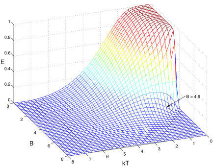
FIG. 1.: We have plotted the entanglement $E$ between two qubits interacting according to the antiferromagnetic Heisenberg model as a function of the external field $B$ and temperature (multiplied by the Boltzmann’s constant) $kT$ with coupling $J=1$. The $B=4.6$ line pointed out in the figure shows that for certain values of $B$ it is possible to increase $E$ by increasing $T$. At $T=0$, $E$ has a sharp transition from $1$ to $0$ as $B$ crosses the critical value of $B_{c}=4$. $E$ always becomes zero for values of $T$ exceeding $T_{c}=8/k\ln 3$

We first examine the $2$ qubit antiferromagnetic chain. We will use the entanglement of formation [5, 16, 17] to calculate the entanglement of the two qubits. To calculate this entanglement measure, starting from the density matrix $\rho$, we first need to define the product matrix $R$ of the density matrix and its time-reversed matrix

$$R\equiv\rho(\sigma_{y}\otimes\sigma_{y})\rho^{*}(\sigma_{y}\otimes\sigma_{y}).$$ (2)

Now concurrence is defined by

$$C=max\{\lambda_{1}-\lambda_{2}-\lambda_{3}-\lambda_{4},0\}$$ (3)

where the $\lambda_{i}$ are the square roots of the eigenvalues of $R$, in decreasing order. In this method the standard basis, $\{|00\rangle,|01\rangle,|10\rangle,|11\rangle\}$ must be used. The entanglement of formation is a strictly increasing function of concurrence, thus there is a one-to-one correspondence. The amount of entanglement in our special case is given by

$$E = -(\frac{1+\sqrt{1-C^{2}}}{2})\log_{2}{(\frac{1+\sqrt{1-C^{2}}}{2})}$$ (4)

$$- (\frac{1-\sqrt{1-C^{2}}}{2})\log_{2}{(\frac{1-\sqrt{1-C^{2}}}{2})},$$ (5)

where $C$ is the concurrence given by

$$C = 0~{}\text{if}~{}e^{8J/kT}\leq 3,$$ (6)

$$= \frac{e^{8J/kT}-3}{1+e^{-2B/kT}+e^{2B/kT}+e^{8J/kT}}~{}\text{if}~{}e^{8J/kT}>3.$$ (7)

Fig.1 shows the plot of this entanglement as a function of magnetic field and temperature.

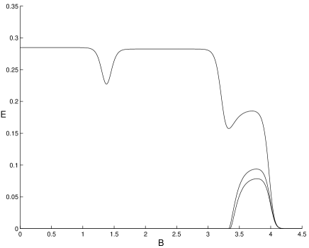
FIG. 2.: The topmost plot shows the variation of nearest neighbor entanglement $E$ with $B$ for $N=6$, $kT=0.1$ and $J=1$. The middle and the bottom most plot show the same for next nearest and next to next nearest neighbors respectively. The reason for the shapes of the curves is presented in the text. Note that $l_{E}$ is $1$ lattice spacing for all values of $B$ below $B_{E}=3.24$ and changes to $3$ lattice spacings for a range of $B$ after $B_{E}$. This means one can magnetically tune in the entanglement between any two qubits by increasing $B$. We also see the decay of all types of entanglement shortly after $B=B_{c}=4$.

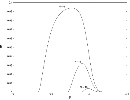
FIG. 3.: We have plotted the variation of next to nearest neighbor entanglement $E$ with $B$ at $kT=0.1$ and $J=1$ for three values of $N$. We see that greater the $N$, a larger value of $B$ is needed to tune in this entanglement, which is absent until $B$ reaches a certain value. However, this entanglement disappears irrespective of $N$ shortly after B exceeds $B_{c}=4$.

For $B=0$, the singlet is the ground state and the triplets are the degenerate excited states. In this case, the maximum entanglement is at $T=0$ and it decreases with $T$ due to mixing of the triplets with the singlet. For a higher value of $B$, however, the triplet states split, and $|00\rangle$ becomes the ground state. In that case there is no entanglement at $T=0$, but increasing $T$ increases entanglement by bringing in some singlet component into the mixture. On the other hand, as $B$ is increased at $T=0$, the entanglement vanishes suddenly as $B$ crosses a critical value of $B_{c}=4J$ when $|00\rangle$ becomes the ground state. This special point $T=0,B=B_{c}$, at which entanglement undergoes a sudden change with variation of $B$, is the point of a quantum phase transition [21](phase transitions taking place at zero temperature due to variation of interaction terms in the Hamiltonian of a system). At any finite $T$, however, entanglement decays off analytically after $B$ crosses $B_{c}$. In the ferromagnetic case, the state of the system at $B=0$ and $T=0$ is an equal mixture of the three triplet states. This state is disentangled [7]. Increasing $B$ increases the proportion of $|00\rangle$ in the state which cannot make it entangled. Increasing $T$ increases the proportion of singlet in the state which can only decrease entanglement by mixing with the triplet. Thus we never find any entanglement in the $2-$qubit ferromagnet. These features of the $2-$qubit Heisenberg model are also present in the $N$ qubit model (which we investigate numerically) along with additional features, which we describe next.

We first plot (Fig.2) how the entanglement between nearest, next nearest and next to next nearest neighbors in an antiferromagnet vary with $B$ for a finite but low $T$ (so that the entanglement is predominantly determined by the ground state). For the nearest neighbor entanglement there are dips in the entanglement at certain points. These dips are due to the mixing of two different entangled ground states at these points. After exceeding a certain value of $B$ (say, $B_{E}$, which might depend on $N$), an equal superposition of states with only one spin up becomes the ground state. This state $|\Psi_{\mbox{sym}}\rangle=\frac{1}{\sqrt{N}}(|100...0\rangle+|010...0\rangle+...+|000...1\rangle)$ has entanglement between any two pairs. Thus we see the next nearest and the next to next nearest neighbor entanglement becoming finite only after $B$ crosses $B_{E}$. One can call this entanglement between non nearest neighbors magnetic entanglement as it is brought about by increasing $B$. When $B$ is increased further, beyond a critical value $B_{c}=2J\{1+\frac{1+(-1)^{N}}{2}+\frac{1-(-1)^{N}}{2}\cos{\pi/N}\}\leq 4J$ the disentangled state $|00...0\rangle$ becomes the ground state. At precisely $T=0$, crossing $B_{c}$ ensures the complete vanishing of all types of entanglement. For finite $T$, all types of entanglement decay to zero gradually after $B_{c}$. This is illustrated in Fig.3. An interesting point, shown by all our numerical evidence, is that the change in entanglement $\Delta E$ at constant temperature due to change in $B$, can never exceed $|\Delta B|/kT$. This might not be surprising as entanglement is an entropic quantity and $|\Delta B|$ is the change in internal energy.

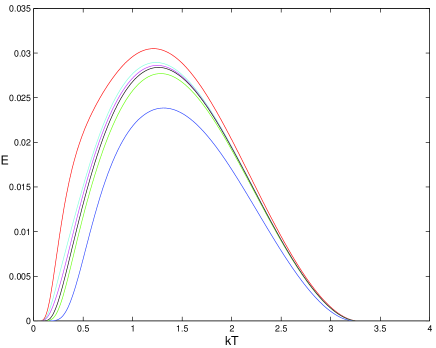
FIG. 4.: The nearest neighbor entanglement $E$ is plotted as a function of $kT$ at $B=4.2$, $J=1$ and various values of $N$ (from top to bottom, $N=6,N=8,N=10,N=9,N=7$ and $N=5$). This graph shows that $E$ of even $N$ states decreases, $E$ of odd $N$ states increases with $N$ and they both tend to merge with each other for high $N$ (they almost coincide for $N=9$ and $N=10$). The plot also illustrates that one can increase the entanglement by increasing $T$.

If we define a quantity called the entanglement length $l_{E}$ as the smallest separation between qubits beyond which the entanglement disappears, then for a small range of $B$ after crossing $B_{E}$, $l_{E}$ becomes equal to the farthest neighbor separation (i.e it can be made arbitrarily large). We have checked this numerically upto $N=13$, and it is reasonable to conjecture that this will be true for any $N$. If this conjecture is false, it will still be interesting to find the value of $N$ beyond which you can never increase $l_{E}$ to the largest neighbor separation. Of course, as evident from Fig.2, the further the qubits are, lesser is the magnitude of the entanglement between them. Note that the above definition of entanglement length differs from that defined in Ref.[22] where quantum to classical transitions in noisy quantum computers was studied (see also Ref.[23] for transitions in quantum networks).

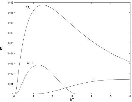
FIG. 5.: This graph shows the variation of total mutual information with temperature for the antiferromagnetic (AF,I) and ferromagnetic (F,I) case for $N=10$, $B=4.2$ and $|J|=1$. The entanglement for the antiferromagnetic case (AF, E) is also plotted for a comparison.

As mentioned earlier, $|\Psi_{\mbox{sym}}\rangle$ becomes the ground state for a certain range of values of the external magnetic field (confirmed numerically up to $N=13$ and conjectured for other values of $N$). At extremely low temperatures and appropriate magnetic fields, thus, the state of the chain will almost be $|\Psi_{\mbox{sym}}\rangle$. This state has the interesting property that there exists entanglement between any two qubits. The reduced density matrix of any two spins in the state $|\Psi_{\mbox{sym}}\rangle$ is $\rho=\frac{2}{N}|\Psi^{+}\rangle\langle\Psi^{+}|+(1-\frac{2}{N})|00\rangle\langle 00|$ where $|\Psi^{+}\rangle=\frac{1}{\sqrt{2}}(|01\rangle+|10\rangle)$. This is an entangled state. For any $N$, if we measure the state of all qubits except two, those two qubits would be projected onto a maximally entangled state, which can then be verified through Bell-CHSH inequalities [24]. Even for any other mixed state which may thermally or magnetically generated, there exists A neccessary and sufficient condition to check whether the CHSH inequality is violated [24]. Of course, one has to make an appropriate choice of measurement axes on the two spins in the solid. As different components of the magnetic susceptibility tensor are proportional to spin-spin correlations in different pairs of directions [21], a CHSH inequality can tested by measuring different components of the magnetic susceptibility tensor .

We now look at the dependence of entanglement on $T$ in the $N$ qubit case for a fixed $B$. Fig.4 shows that one can increase entanglement by increasing $T$. After a certain $T$, all entanglement dies out. In all simulations we find this temperature to be lower than $T_{c}=8/\ln 3$. Also, we see that the curves for entanglement in the case of even and odd $N$ approach each other as $N$ increases. This seems reasonable because for large $N$, it should not make a difference to the nearest neighbor entanglement whether we add or subtract a qubit somewhere far in the chain. As with the 2-qubit case, we find no thermal or magnetic entanglement in a ferromagnetic chain.

We would now like to compare the amount of entanglement in the solid to the total two qubit correlations. An information theoretic measure of these correlations is the mutual information given by $I(i:j)=S(\rho^{i})+S(\rho^{j})-S(\rho^{ij})$ where $\rho^{i}$, $\rho^{j}$ are the density matrices of the $i$th and the $j$th spin respectively, $\rho^{ij}$ is their joint state and $S(\rho)$ represents the entropy of $\rho$. In a manner similar to the connected correlation function [26], this quantity measures the effect that genuinely results from the interaction between particles. A plot of $I(i:j)$ with temperature is shown in Fig.5. It is interesting to note that though entanglement is always absent in a ferromagnet, $I$ for nearest neighbors (stemming entirely from classical correlations) can be increased by increasing the temperature. It is well known that the magnetic susceptibility is proportional to the spin-spin correlations [15]. It would be interesting to investigate whether any difference arises between the antiferromagnetic and ferromagnetic susceptibility tensors due to the complete absence of entanglement in the latter case.

In this letter, we have introduced the concepts of thermal and magnetic entanglement and analyzed their behaviour in the $1$D isotropic Heisenberg model. We have found critical values of field beyond which entanglement disappears at zero temperature and declines at finite temperature. Our results indicate that there is also a critical temperature after which all entanglement vanishes, though there is a range of field in which entanglement can be increased by increasing the temperature. Based on numerical evidence, we have conjectured that the entanglement length can be made arbitrarily large by applying an appropriate external magnetic field. We have also compared the total correlations to the entanglement. Our work raises a number of interesting questions and conjectures to prove and the possibility of numerous generalizations such as higher dimensions, non nearest neighbor interactions, anisotropies, other Hamiltonians and so on. In addition, we also showed that by applying a suitable magnetic field and lowering the temperature sufficiently, and doing suitable projections, one can create a state which violates the Bell’s inequalities. The ”natural” entanglement can be verified in these cases. In future we will investigate how to map this natural entanglement out of the solid (eg. by neutron scattering) and use it as a resource in communications.

We thank M. Bourenanne and V. Kendon for useful discussions. After completion of the article M. Nielsen brought our attention to the fact that the two qubit case has been considered previously by him in [25]. Funding by the European Union project EQUIP (contract IST-1999-11053) and Hewlett Packard is acknowledged. MCA acknowledges funding from George F. Smith through the Associates SURF endowment. VV acknowledges hospitality of the Erwin Schrödinger Institute in Vienna where part of the work was carried out.

REFERENCES

- [1] A. Einstein, B. Podolsky and N. Rosen, Phys. Rev. 47, 777 (1935).
- [2] E. Schrödinger, Naturwissenschaften 23, 807 (1935).
- [3] J. S. Bell, Physics 1, 195 (1964).
- [4] C. H. Bennett and D. P. DiVincenzo, Nature 404, 247 (2000).
- [5] C. H. Bennett, D. P. DiVincenzo, J. A. Smolin and W. K. Wootters, Phys. Rev. A 54, 3824 (1996).
- [6] V. Vedral, M. B. Plenio, M. A. Rippin and P. L. Knight, Phys. Rev. Lett. 78, 2275 (1997).
- [7] V. Vedral and M. B. Plenio, Phys. Rev. A 57, 1619 (1998).
- [8] B. E. Kane, Nature 393, 133 (1998).
- [9] D. C. Mattis, The theory of magnetism, (Harper and Row, 1965).
- [10] C. J. Thompson in Phase transitions and critical phenomena, C. Domb and M. S. Green eds. (Academic Press, London 1972).
- [11] P. R. Hammar et al., Phys. Rev. B 59, 1008 (1999).
- [12] H. A. Bethe, Z. Physik 71, 205 (1931).
- [13] J. Bonner and M. E. Fisher, Phys. Rev. 135, A640 (1964).
- [14] C. N. Yang and C. P. Yang, Phys. Rev. 150, 327 (1966).
- [15] S. Eggert, I. Affleck and M. Takahashi, Phys. Rev. Lett. 73, 332 (1994).
- [16] W. K. Wootters, Phys. Rev. Lett 80, 2245 (1998).
- [17] V. Coffman, J. Kundu and W. K. Wootters, Phys. Rev. A 61, 052306 (2000).
- [18] W. K. Wootters, Entangled chains, quant-ph/0001114.
- [19] K. M. O’Connor and W. K. Wootters, Entangled rings, quant-ph/0009041.
- [20] H. J. Briegel and R. Raussendorf, Persistent entanglement in arrays of interacting qubits, quant-ph/0004051.
- [21] S. Sachdev, Quantum phase transitions (Cambridge University Press, Cambridge, 1999).
- [22] D. Aharonov, A quantum to classical phase transition in a noisy quantum computer, quant-ph/9910081.
- [23] P. Torma, Phys. Rev. Lett. 81, 2185 (1998).
- [24] R. Horodecki, P. Horodecki and M. Horodecki, Phys. Lett. A 200 340 (1995).
- [25] M. A. Nielsen, PhD Thesis, University of New Mexico (1998), quant-ph/0011036.
- [26] J. J. Binney et al., The theory of critical phenomena, (Clarendon Press, Oxford, 1992).