Self-Consistency
of Thermal Jump Trajectories

Summary.

It is problematic to interpret the quantum jumps of an atom interacting with thermal light in terms of counts at detectors monitoring the atom’s inputs and outputs. As an alternative, we develop an interpretation based on a self-consistency argument. We include one mode of the thermal field in the system Hamiltonian and describe its interaction with the atom by an entangled quantum state while assuming that the other modes induce quantum jumps in the usual fashion. In the weak-coupling limit, the photon number expectation of the selected mode is also seen to execute quantum jumps, although more generally, for stronger coupling, Rabi oscillations are observed; the equilibrium photon number distribution is a Bose-Einstein distribution. Each mode may be viewed in isolation in a similar fashion, and summing over their weak-coupling jump rates returns the net jump rates for the atom assumed at the outset.

1 Introduction

The notion of a quantum jump entered physics with Bohr’s model of the atom and was elaborated in a semi-quantitative formulation in Einstein $A$ and $B$ theory einstein16 . It was, from the beginning, an idea at variance with the usual commitment to a continuous time evolution and with the continuous constitution of light as an electromagnetic wave. The appearance of the Schrödinger equation relieved the situation somewhat, but ultimately, through the use of perturbation theory to make testable predictions about quantum scattering processes, the quantum jump remains with us, though certainly in a more sophisticated and mathematically refined form.

The Monte-Carlo wavefunction and quantum trajectory methods developed in quantum optics dalibard92 ; dum92 ; carmichael93 use quantum jumps as an explicit component of a stochastic time evolution in a manner very reminiscent of Einstein $A$ and $B$ theory. In fact, the only novelty is to combine Einstein’s rules for quantum jumps with a coherent evolution between jumps that admits a dynamic involving superpositions of stationary states. In this, these methods achieve something remarkably similar to the proposal of Bohr, Kramers, and Slater (BKS) bohr24 ; slater24 for uniting discontinuous jumps among the stationary states of a material system with a continuous evolution between jumps, during which time material oscillators, possessing coherent amplitudes, are brought into play.

The realistic interpretation sought by BKS may not, however, be entertained. In most circumstances, an interpretation of the jumps employed in quantum trajectory theory is based upon a record of time-resolved photon counts which might be realized in practice by terminating every output channel in a photodetector carmichael93 ; carmichael99 . This scenario is plausible because optical frequencies are sufficiently high that scattered photons can be detected against an essentially vacuum-state background. The measurement-based interpretation is problematic, though, for an atom exchanging photons with a thermal environment. In this situation, incoherent photons are both emitted and absorbed; moreover, it is impossible to distinguish a scattered photon from some other photon in the environment. Of course, schemes such as electron shelving exist that are able to monitor thermal quantum jumps nagourney86 ; sauter86 ; bergquist86 . They, however, make intrusive measurements by utilizing strong couplings to other inputs and outputs, and are not a suitable foundation for the interpretation of quantum trajectory equations. The relationship, in fact, is exactly the reverse; electron shelving is one of the measurement schemes that quantum trajectories would propose to explain.

In this paper we follow a different direction to give substance, beyond a mere assertion, to the interpretation that an atom exchanging photons with a thermal environment does, in some well-defined sense, execute jumps. We define the sense through a self-consistency argument. Contrary to the notion of quantum jumps, quantum mechanics continuously entangles two interacting systems through the Schrödinger evolution. We show that a single mode, selected from the many modes of a thermal environment, and allowed to evolve in interacting with an atom to produce such an entanglement, is, in fact, seen to undergo jumps in its photon number expectation if it is assumed that all other modes of the environment, treated collectively as a reservoir, induce jumps between the atomic states according to the rules of Einstein theory. The jump evolution for the selected mode emerges from an otherwise continuous evolution in the weak-coupling limit. Thus, assuming jumps induced by the reservoir as a whole leads, self-consistently, to the appearance of jumps in an individual mode of the reservoir when that mode is allowed to entangle with the atom via the standard interaction Hamiltonian and Schrödinger evolution. The jumps do bring the individual mode to a Bose-Einstein distribution over photon number, and the jump rates, derived for every mode viewed individually in this way, sum to net rates which agree with Einstein $A$ and $B$ theory.

The underlying theme of this paper is the conflict between a continuous and a discontinuous quantum evolution and the self-consistency of the two in the perturbative weak-coupling limit. We therefore briefly review, in Sect. 2, the quantum jump model of Einstein, the BKS proposal to include a continuous evolution, and the quantum trajectory realization of the latter. The argument for the self-consistency of thermal jump trajectories is elaborated in Sect. 3.

2 Einstein $A$ and $B$ Theory, BKS, and Quantum Trajectories

2.1 Thermal Quantum Jumps

We consider the single two-state atom illustrated in Fig. 1, in thermal equilibrium with Planck radiation at temperature $T$. In Einstein $A$ and $B$ theory photons are exchanged between the atom and the radiation field as the atom jumps randomly between its two stationary states. The jump rates follow a prescription taking into account spontaneous emission, stimulated emission, and absorption, with einstein16

$$\halign to=433.62pt{\@eqnsel\hskip\@centering$\displaystyle{#}$&\global\@eqcnt\@ne\hskip 2\arraycolsep\hfil${#}$\hfil&\global\@eqcnt\tw@\hskip 2\arraycolsep$\displaystyle{#}$\hfil&\llap{#}\cr 0.0pt plus 1000.0pt$\displaystyle{\Gamma_{\rm down}&10.0pt\hfil${=&10.0pt$\displaystyle{A+B\sigma(\omega_{0})\;, {}&\hbox to0.0pt{\hss{\rm(0.1a)}\cr\penalty 100\vskip 3.0pt\vskip 0.0pt\cr 0.0pt plus 1000.0pt$\displaystyle{\Gamma_{\rm up}&10.0pt\hfil${=&10.0pt$\displaystyle{B\sigma(\omega_{0})\;, &\hbox to0.0pt{\hss{\rm(0.1b)}\cr}}}}}}}}}$$

where

$$\sigma(\omega_{0})=\bar{n}(\omega_{0})\hbar\omega_{0}[\rho(\omega_{0})/V]$$ (2)

is the energy density of the radiation field at the resonance frequency $\omega_{0}$ of the atom, with average photon number per mode

$$\bar{n}(\omega_{0})=[e^{\hbar\omega_{0}/k_{B}T}-1]^{-1}$$ (3)

and mode density (in volume $V$)

$$\rho(\omega_{0})=\frac{\omega_{0}^{2}V}{\pi^{2}c^{3}}\;,$$ (4)

and the Einstein $A$ and $B$ coefficients must satisfy

$$\frac{B}{A}=\frac{\pi^{2}c^{3}}{\hbar\omega_{0}^{3}}$$ (5)

in order for the atom to be brought into thermal equilibrium with the radiation.

[width=.3]sctj1.eps

Figure 1: Thermal quantum jumps in Einstein $A$ and $B$ theory. The jump rates are defined in (2.1) and (2.1).

With the help of the relationship (5), we write (2.1) and (2.1) in the modern notation

$$\halign to=433.62pt{\@eqnsel\hskip\@centering$\displaystyle{#}$&\global\@eqcnt\@ne\hskip 2\arraycolsep\hfil${#}$\hfil&\global\@eqcnt\tw@\hskip 2\arraycolsep$\displaystyle{#}$\hfil&\llap{#}\cr 0.0pt plus 1000.0pt$\displaystyle{\Gamma_{\rm down}&10.0pt\hfil${=&10.0pt$\displaystyle{A[\bar{n}(\omega_{0})+1]\;, {}&\hbox to0.0pt{\hss{\rm(0.6a)}\cr\penalty 100\vskip 3.0pt\vskip 0.0pt\cr 0.0pt plus 1000.0pt$\displaystyle{\Gamma_{\rm up}&10.0pt\hfil${=&10.0pt$\displaystyle{A\bar{n}(\omega_{0})\;. &\hbox to0.0pt{\hss{\rm(0.6b)}\cr}}}}}}}}}$$

Einstein theory does not assign a value to the coefficient $A$. From quantum mechanics, however, using Fermi’s Golden rule we obtain

$$A=2\pi\sum_{\lambda}\int\!d\Omega\,\rho(\omega_{0})|\kappa_{\lambda,\hat{\vec{n}}}(\omega_{0})|^{2}\;,$$ (7)

where

$$|\kappa_{\lambda,\hat{\vec{n}}}(\omega_{0})|=\sqrt{\frac{\omega_{0}}{2\pi\epsilon_{0}V}}|\hat{e}_{\lambda,\hat{\vec{n}}}\cdot\vec{d}_{eg}|$$ (8)

is the dipole coupling strength to a mode of the radiation field with polarization $\lambda$ and direction of propagation specified by the unit vector $\hat{\vec{n}}$ (polarization vector $\hat{e}_{\lambda,\hat{\vec{n}}}$); $\vec{d}_{eg}$ is the atomic dipole matrix element.

Commonly, Einstein theory is discussed at the level of rate equations for the occupation probabilities of the atomic stationary states. The theory does, however, define a stochastic process – one that may be visualized in terms of quantum jumps whose occurrences unfold randomly in time. With each realization of the stochastic process we associate a record of jump types and jump times,

$${\rm REC}\equiv\left\{\matrix{\ldots&\Gamma_{\rm down}&\Gamma_{\rm up}&\Gamma_{\rm down}&\Gamma_{\rm up}&\Gamma_{\rm down}&\ldots\cr\ldots&t+\tau_{1}&t+\tau_{2}&t+\tau_{3}&t+\tau_{4}&t+\tau_{5}&\ldots}\right.\;.$$ (9)

In Fig. 2 we illustrate the discontinuous evolution of the atom in coordination with its absorption and emission of thermal photons.

[width=.6]sctj2.eps

Figure 2: Sample realization of the Einstein stochastic process. The corresponding record is defined in (9).

2.2 Coherence: The BKS Proposal

Although Bohr had himself put forward the notion of a quantum jump to explain the association of stationary-state energy differences with electromagnetic wave frequencies in his model of the hydrogen atom, he became quite dissatisfied with the idea in the concrete form it acquired under Einstein’s proposal. It was the light quantum, specifically, that troubled him the most. Bohr insisted that since so many optical phenomena rely on the continuity of coherent waves, the wave nature of light simply could not be dismissed. He recognized, on the other hand, that a discontinuous process was definitely needed to account for light emission and detection. What he was unavoidably drawn towards, then, was some sort of merging of the two ideas.

A program to accomplish this was outlined in what has come to known as the BKS proposal bohr24 ; slater24 . The central idea of this proposal is the proposition that during the residence times in a stationary state, represented by the horizontal lines in Fig. 2, an atom is not inactive in its interaction with the electromagnetic field; rather, it acts through a coherent dipole radiator, or “virtual oscillator” in the words of BKS, which is all the time radiating an electromagnetic wave of frequency $\omega_{0}=(E_{e}-E_{g})/\hbar$. This wave is either in phase or out of phase with the external radiation at frequency $\omega_{0}$ depending on whether the residence is in the stationary state with energy $E_{e}$ or $E_{g}$. Thus, there is an energy transfer under the laws of classical electrodynamics either to the electromagnetic field from the dipole, or in the reverse direction, depending on the stationary state note1 . Clearly a double counting of the exchanged energy occurs if one accepts that light quanta are also emitted and absorbed at the times of the jumps. However, the goal was precisely to eliminate these quanta, although still permitting the atom to jump. BKS attempted, thus, to retain, but keep separate, two incompatible mechanisms for energy exchange – a wave (continuous) mechanism for the absorption and emission of radiation and a particle (discontinuous) mechanism for the change of material state energies. Their proposal foundered on its obvious violation of energy conservation at the level of the individual quantum events, a feature that appeared not to be supported in Compton scattering experiments bothe25 ; compton25 .

2.3 Coherence: Quantum Trajectories

In retrospect we can see that Bohr had in mind a conception of light that, although supported by numerous wave phenomena in optics, was largely inappropriate for the light sources available at the time. Radiators in thermal equilibrium are not sources of coherent waves. They radiate electromagnetic noise, which, with filtering, can approximate low intensity light possessing first-order coherence, but is very far from the classical concept of a coherent wave of large and adjustable amplitude. Modern lasers, however, emit something close to the classical ideal. In their case, the high coherence, if it is to be preserved, disallows the tracking of energy at the level of the individual quanta, so that the energy conservation argument against the BKS proposal does not apply.

Quantum trajectory theory is designed to deal with problems involving the interaction of matter with the high coherence light sources available in modern laboratories. It shows remarkable similarities to the BKS proposal. These are described elsewhere carmichael97 ; carmichael99 , and we do not plan to discuss them in any depth here. As an introduction to our main topic, however, it is useful to contrast Einstein $A$ and $B$ theory with the quantum trajectory description of a coherent field, amplitude ${\cal E}$, resonantly exciting the two-state atom of Fig. 1. The connections with BKS emerge automatically through this exercise.

The atom is still located in a thermal environment and quantum jumps still appear as they do in Fig. 2 – but with one notable modification. Due to the induced coherence, it is necessary that the system state be a superposition of the stationary states $|E_{e}\rangle$ and $|E_{g}\rangle$, which we denote by $|\psi_{\rm REC}(t)\rangle$. As suggested by BKS, there is a coherent interaction with the electromagnetic field between the quantum jumps. This we account for by a continuous evolution under the Schrödinger equation dalibard92 ; dum92 ; carmichael93 (for the unnormalized conditional state)

$$\frac{d|\bar{\psi}_{\rm REC}\rangle}{dt}=\frac{1}{i\hbar}\hat{H}_{B}|\bar{\psi}_{\rm REC}\rangle\;,$$ (10)

with non-Hermitian Hamiltonian

$$\hat{H}_{B} = {\textstyle{1\over 2}\displaystyle}\hbar(\omega_{0}-i\Gamma_{\rm down})|E_{e}\rangle\langle E_{e}|-{\textstyle{1\over 2}\displaystyle}\hbar(\omega_{0}+i\Gamma_{\rm up})|E_{g}\rangle\langle E_{g}|$$ (12)

$$+i\hbar{\cal E}(e^{i\omega_{0}t}|E_{g}\rangle\langle E_{e}|-e^{-i\omega_{0}t}|E_{e}\rangle\langle E_{g}|)\;,$$

in which the external coherent field is classical, and its interaction with the atom is treated in the dipole and rotating-wave approximations. The quantum jumps are governed by the probabilistic rules of Einstein $A$ and $B$ theory, generalized, in a natural way, to account for the fact that the system at any time is not definitely in a particular stationary state. There are jumps

$$\halign to=433.62pt{\@eqnsel\hskip\@centering$\displaystyle{#}$&\global\@eqcnt\@ne\hskip 2\arraycolsep\hfil${#}$\hfil&\global\@eqcnt\tw@\hskip 2\arraycolsep$\displaystyle{#}$\hfil&\llap{#}\cr 0.0pt plus 1000.0pt$\displaystyle{|\bar{\psi}_{\rm REC}\rangle&10.0pt\hfil${\raise 5.0pt\hbox{$\matrix{{}_{\Gamma_{\rm down}}\cr\vskip-3.0pt\cr\to}$}&10.0pt$\displaystyle{(|E_{g}\rangle\langle E_{e}|)|\bar{\psi}_{\rm REC}\rangle\;,{}&\hbox to0.0pt{\hss{\rm(0.13a)}\cr\penalty 100\vskip 3.0pt\vskip 0.0pt\cr\vskip-2.0pt\cr 0.0pt plus 1000.0pt$\displaystyle{|\bar{\psi}_{\rm REC}\rangle&10.0pt\hfil${\raise 5.0pt\hbox{$\matrix{{}_{\Gamma_{\rm up}}\cr\vskip-3.0pt\cr\to}$}&10.0pt$\displaystyle{(|E_{e}\rangle\langle E_{g}|)|\bar{\psi}_{\rm REC}\rangle\;, &\hbox to0.0pt{\hss{\rm(0.13b)}\cr}}}}}}}}}$$

with jump rates

$$\halign to=433.62pt{\@eqnsel\hskip\@centering$\displaystyle{#}$&\global\@eqcnt\@ne\hskip 2\arraycolsep\hfil${#}$\hfil&\global\@eqcnt\tw@\hskip 2\arraycolsep$\displaystyle{#}$\hfil&\llap{#}\cr 0.0pt plus 1000.0pt$\displaystyle{R_{\rm down}&10.0pt\hfil${=&10.0pt$\displaystyle{\Gamma_{\rm down}|\langle E_{e}|\psi_{\rm REC}\rangle|^{2}\;,{}&\hbox to0.0pt{\hss{\rm(0.14a)}\cr\penalty 100\vskip 3.0pt\vskip 0.0pt\cr 0.0pt plus 1000.0pt$\displaystyle{R_{\rm up}&10.0pt\hfil${=&10.0pt$\displaystyle{\Gamma_{\rm up}|\langle E_{g}|\psi_{\rm REC}\rangle|^{2}\;. &\hbox to0.0pt{\hss{\rm(0.14b)}\cr}}}}}}}}}$$

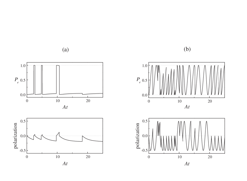
Figure 3: Sample quantum trajectories with both thermal jumps and induced coherence: $\bar{n}(\omega_{0})=0.25$, ${\cal E}/A=0.1$ and $1.5$ [(a) and (b)].

Figure 3 illustrates how realizations of this stochastic process appear. In (a) the coherent excitation is relatively weak and the overall form of the evolution remains close to that produced by the Bohr-Einstein quantum jumps (Fig. 2). There is, however, in addition to the switching of the energy, a weak induced coherence carried along by the continuous evolution between jumps as a nonvanishing polarization amplitude, quite reminiscent of the BKS virtual oscillator. In Fig. 3(b) the coherent excitation is much stronger. Here, the dominant mechanism for evolution between the stationary states is a coherent Rabi oscillation; we move to a coherent evolution that is nonperturbative and a regime which only became accessible with the invention of the laser. This, specifically, is a form of evolution following from the Schrödinger equation; nonperturbative coherence was not anticipated by the BKS proposal. We might note in passing that lasing without inversion and related phenomena acquire their counterintuitive features from such nonperturbative coherence carmichael97 .

3 Self-Consistency of Thermal Quantum Jumps

At a sufficiently low temperature, when $\bar{n}(\omega_{0})\ll 1$, the jump record that labels the state can reasonably be made by detectors monitoring the scattered light. Almost all jumps will be down-jumps governed by the spontaneous emission rate $A$ which may be identified with emitted photons counted as isolated (in space and time) excitations of the vacuum. For many applications in quantum optics this is the situation in reality. Nonetheless, the thermal jumps, though they might be negligible in practice, cannot be set aside from a fundamental point of view. Considering then those jumps which cannot reasonably be identified with the “click” of a detector, is there any other justification for returning to the language of the old quantum theory, given that, in quantum mechanics, the Schrödinger equation invokes only a continuous evolution? We aim to show that there is, in so far as the jumps are self-consistent – consistent with the Schrödinger evolution – in the weak-coupling limit.

3.1 Trajectories for a Single Field Mode

The Hamiltonian for a two-state atom interacting with the radiation field of a thermal environment (we now take ${\cal E}=0$) is

$$\hat{H} = {\textstyle{1\over 2}\displaystyle}\hbar\omega_{0}|E_{e}\rangle\langle E_{e}|-{\textstyle{1\over 2}\displaystyle}\hbar\omega_{0}|E_{g}\rangle\langle E_{g}|$$ (17)

$$+\sum_{\lambda^{\prime},\hat{\vec{n}}^{\prime},\omega^{\prime}}\hbar\omega^{\prime}\hat{r}^{\dagger}_{\lambda^{\prime},\hat{\vec{n}}^{\prime},\omega^{\prime}}\hat{r}_{\lambda^{\prime},\hat{\vec{n}}^{\prime},\omega^{\prime}}$$

$$+\sum_{\lambda^{\prime},\hat{\vec{n}}^{\prime},\omega^{\prime}}\hbar[\kappa_{\lambda^{\prime},\hat{\vec{n}}^{\prime}}(\omega^{\prime})|E_{e}\rangle\langle E_{g}|\hat{r}_{\lambda^{\prime},\hat{\vec{n}}^{\prime},\omega^{\prime}}+{\rm H.c.}]\;,$$

where $\hat{r}^{\dagger}_{\lambda,\hat{\vec{n}},\omega}$ and $\hat{r}_{\lambda,\hat{\vec{n}},\omega}$ are creation and annihilation operators for the field mode with polarization $\lambda$, propagation direction $\hat{\vec{n}}$, and frequency $\omega$, and $\kappa_{\lambda,\hat{\vec{n}}}(\omega)$ is the mode coupling coefficient whose magnitude is defined in (8). The stochastic process (10)–(2.3) (${\cal E}=0$) is developed, formally, around the master equation derived from (17) dalibard92 ; dum92 ; carmichael93 . This master equation describes the quantum state of the atom alone, after tracing over every mode of the radiation field. Our idea is to raise one mode of the field to the same status as the atom by including it, along with its interaction with the atom, in the system Hamiltonian. All other modes are to be treated as a reservoir as before and their interaction with the atom described by quantum jumps. The stochastic process is the same as in (10)–(2.3), but with the non-Hermitian Hamiltonian $\hat{H}_{B}$ replaced by

$$\hat{H}_{B} = {\textstyle{1\over 2}\displaystyle}\hbar(\omega_{0}-i\Gamma_{\rm down})|E_{e}\rangle\langle E_{e}|-{\textstyle{1\over 2}\displaystyle}\hbar(\omega_{0}+i\Gamma_{\rm up})|E_{g}\rangle\langle E_{g}|$$ (20)

$$+\hbar\omega\hat{r}^{\dagger}_{\lambda,\hat{\vec{n}},\omega}\hat{r}_{\lambda,\hat{\vec{n}},\omega}$$

$$+\hbar[\kappa_{\lambda,\hat{\vec{n}}}(\omega)|E_{e}\rangle\langle E_{g}|\hat{r}_{\lambda,\hat{\vec{n}},\omega}+{\rm H.c.}]\;.$$

Of course removing one mode from the reservoir has no effect on the overall jump rates for the atom. The change is that we can now follow the evolution of an explicit Hilbert space vector for the selected mode, one that entangles this mode with the atom. We ask how does the selected mode evolve in the Hilbert space; in particular, does it also experience quantum jumps?

Figures 4 and 5 show sample trajectories for the selected-mode photon number expectation note2 – for a series of decreasing coupling strengths, (a)–(d), and assuming resonance with the atom, Fig. 4, and a detuning from the atom, Fig. 5. With the coupling strong compared to the Einstein $A$ coefficient coherent Rabi oscillations are seen. There are also discontinuous changes, which in the case of strong coupling are merely a direct manifestation of the assumed quantum jumps for the atom. Note, however, that the atom does not jump monotonously, “up” then “down” then “up” $\cdots$, as in Fig. 2; repeated up-jumps can transfer many energy quanta to the field mode. At an intermediate coupling strength, partial Rabi oscillations are still present. Once the coupling becomes weak, though, the Rabi oscillations apparently disappear altogether, and an entirely new kind of jump evolution sets in. These jumps proceed at a rate far less than the overall jump rate for the atom. Their rate decreases with the square of the coupling constant [(c) to (d)] and also when the detuning is increased (from Fig. 4 to Fig. 5).

Having, then, assumed jumps for the atom in interaction with all but one of the field modes, a jump evolution for the one remaining mode emerges naturally in the weak-coupling limit. We close the self-consistent loop by showing that the one mode samples a Bose-Einstein distribution, and by calculating the rate of the single-mode jumps, to demonstrate that the sum over modes returns the rates $\Gamma_{\rm up}$ and $\Gamma_{\rm down}$.

[width=.55]sctj4.eps

Figure 4: Sample trajectories for the photon number expectation of a single field mode included as part of the system. The mode is resonant: $\Delta\omega/A=0$, $\bar{n}(\omega_{0})=1$, and $|\kappa_{\lambda,\hat{\vec{n}}}(\omega_{0})|/A=10$, $1.0$, $0.1$, and $0.01$ [(a), (b), (c), and (d)].

[width=.55]sctj5.eps

Figure 5: Sample trajectories for the photon number expectation of a single field mode included as part of the system. The mode is nonresonant: $\Delta\omega/A=2.0$, $\bar{n}(\omega_{0})=1$, and $|\kappa_{\lambda,\hat{\vec{n}}}(\omega)|/A=10$, $1.0$, $0.1$, and $0.01$ [(a), (b), (c), and (d)].

3.2 Self-Consistency

Let us denote the number of energy quanta shared between the atom and the field mode at time $t$ by $n_{\omega}+1$. Let $t_{k}$ be the time of the very last jump of the atom and $t_{k+1}$ be the time of the jump that is to occur next. Then, for $t_{k}<t<t_{k+1}$, the entangled state of the atom and field mode may be expanded as

$$|\bar{\psi}_{\rm REC}(t)\rangle=\bar{C}_{e|i}(t)|E_{e}\rangle|n_{\omega}\rangle+\bar{C}_{g|i}(t)|E_{g}\rangle|n_{\omega}+1\rangle\;,$$ (21)

with $\bar{C}_{e|i}(0)=\delta_{e,i}$ and $\bar{C}_{g|i}(0)=\delta_{g,i}$, where $i$ is $e$ or $g$ for an up- or down-jump at $t_{k}$, respectively. Writing

$$\halign to=433.62pt{\@eqnsel\hskip\@centering$\displaystyle{#}$&\global\@eqcnt\@ne\hskip 2\arraycolsep\hfil${#}$\hfil&\global\@eqcnt\tw@\hskip 2\arraycolsep$\displaystyle{#}$\hfil&\llap{#}\cr 0.0pt plus 1000.0pt$\displaystyle{\bar{C}_{e|i}(t)&10.0pt\hfil${=&10.0pt$\displaystyle{e^{-i(n_{\omega}+\frac{1}{2})\omega t} e^{i\frac{1}{2}\phi_{\hat{\vec{n}}}(\omega)}\tilde{C}_{e|i}(t)\;,{}&\hbox to0.0pt{\hss{\rm(0.22a)}\cr\penalty 100\vskip 3.0pt\vskip 0.0pt\cr 0.0pt plus 1000.0pt$\displaystyle{\bar{C}_{g|i}(t)&10.0pt\hfil${=&10.0pt$\displaystyle{e^{-i(n_{\omega}+\frac{1}{2})\omega t} e^{-i\frac{1}{2}\phi_{\hat{\vec{n}}}(\omega)}\tilde{C}_{g|i}(t)\;, &\hbox to0.0pt{\hss{\rm(0.22b)}\cr}}}}}}}}}$$

with $\phi_{\hat{\vec{n}}}(\omega)\equiv\arg[\kappa_{\lambda,\hat{\vec{n}}}(\omega)]$, from (10) and (20), the equations of motion for the conditional state amplitudes are

$$\halign to=433.62pt{\@eqnsel\hskip\@centering$\displaystyle{#}$&\global\@eqcnt\@ne\hskip 2\arraycolsep\hfil${#}$\hfil&\global\@eqcnt\tw@\hskip 2\arraycolsep$\displaystyle{#}$\hfil&\llap{#}\cr 0.0pt plus 1000.0pt$\displaystyle{\frac{d{\tilde{C}}_{e|i}}{dt}&10.0pt\hfil${=&10.0pt$\displaystyle{-{\textstyle{1\over 2}\displaystyle} (\Gamma_{\rm down}-i\Delta\omega)\tilde{C}_{e|i}-i|\kappa_{\lambda,\hat{\vec{n}}}(\omega)| \sqrt{n_{\omega}+1}\,\tilde{C}_{g|i}\;, {}&\hbox to0.0pt{\hss{\rm(0.23a)}\cr\penalty 100\vskip 3.0pt\vskip 0.0pt\cr 0.0pt plus 1000.0pt$\displaystyle{\frac{d{\tilde{C}}_{g|i}}{dt}&10.0pt\hfil${=&10.0pt$\displaystyle{-{\textstyle{1\over 2}\displaystyle} (\Gamma_{\rm up}+i\Delta\omega)\tilde{C}_{g|i}-i|\kappa_{\lambda,\hat{\vec{n}}}(\omega)| \sqrt{n_{\omega}+1}\,\tilde{C}_{e|i}\;. &\hbox to0.0pt{\hss{\rm(0.23b)}\cr}}}}}}}}}$$

Consider now the case of an up-jump at $t_{k}$, such that the initial state amplitudes are $\bar{C}_{e|i}(0)=1$ and $\bar{C}_{g|i}(0)=0$. For weak coupling we will have $\bar{C}_{e|i}(t)\approx 1$ and $\bar{C}_{g|i}(t)\sim|\kappa_{\lambda,\hat{\vec{n}}}(\omega)|$, with an overwhelming probability that the next jump of the atom will be a down-jump. By a similar argument, it is highly likely that the down-jump is followed by another up-jump; the most probable progression is then “up”, “down”, “up”, $\ldots$, just as we illustrated it in Fig. 2 (notice that the number $n_{\omega}$ is unchanged throughout such a progression). Due, however, to the small amplitude – either $\bar{C}_{g|i}(t)\sim|\kappa_{\lambda,\hat{\vec{n}}}(\omega)|$ or $\bar{C}_{e|i}(t)\sim|\kappa_{\lambda,\hat{\vec{n}}}(\omega)|$ – excited by the coupling of the atom to the selected mode, there is always a small probability that a jump will occur to break the alternating sequence. An up-jump might be followed by a second up-jump or two down-jumps might occur in a row. These events change $n_{\omega}$ and produce the jumps of the field mode seen in Figs. 4 and 5. In Figs. 4(c) and 5(c), the presence of the small amplitude that underlies the jump mechanism is still seen as a “fuzz” on top of the developing smooth curve. The“fuzz” is even present in Figs. 4(d) and 5(d), though there it is too small to be visible.

The physical interpretation of the anomalous events in the jump record of the atom is that each represents the scattering of a photon between one of the many field modes of the reservoir and the field mode selected to be viewed. Two up-jumps occur in a row for example, because, in the interval between them, the energy absorbed on the first jump is transferred to the selected mode; the quantum trajectory resolves the transfer at the time of the second up-jump.

Our task now is to calculate rates for the unlikely jumps. We do this using the method of Sect. IVD in carmichael97 . The equations of motion (3.2) and (3.2) give

$$\halign to=433.62pt{\@eqnsel\hskip\@centering$\displaystyle{#}$&\global\@eqcnt\@ne\hskip 2\arraycolsep\hfil${#}$\hfil&\global\@eqcnt\tw@\hskip 2\arraycolsep$\displaystyle{#}$\hfil&\llap{#}\cr 0.0pt plus 1000.0pt$\displaystyle{\frac{d|\tilde{C}_{e|i}|^{2}}{dt}&10.0pt\hfil${=&10.0pt$\displaystyle{-\Gamma_{\rm down}|\tilde{C}_{e|i}|^{2} -2|\kappa_{\lambda,\hat{\vec{n}}}(\omega)|\sqrt{n_{\omega}+1}\,{\rm Im} (\tilde{C}_{e|i}\tilde{C}_{g|i}^{*})\;, {}&\hbox to0.0pt{\hss{\rm(0.24a)}\cr\penalty 100\vskip 3.0pt\vskip 0.0pt\cr\vskip 2.0pt\cr 0.0pt plus 1000.0pt$\displaystyle{\frac{d|\tilde{C}_{g|i}|^{2}}{dt}&10.0pt\hfil${=&10.0pt$\displaystyle{-\Gamma_{\rm up}|\tilde{C}_{g|i}|^{2} +2|\kappa_{\lambda,\hat{\vec{n}}}(\omega)|\sqrt{n_{\omega}+1}\,{\rm Im} (\tilde{C}_{e|i}\tilde{C}_{g|i}^{*})\;, {}&\hbox to0.0pt{\hss{\rm(0.24b)}\cr\penalty 100\vskip 3.0pt\vskip 0.0pt\cr\vskip 2.0pt\cr 0.0pt plus 1000.0pt$\displaystyle{\frac{d{\rm Re}(\tilde{C}_{e|i}\tilde{C}_{g|i}^{*})}{dt}&10.0pt\hfil${=&10.0pt$\displaystyle{-{\textstyle{1\over 2} \displaystyle}(\Gamma_{\rm down}+\Gamma_{\rm up}){\rm Re}(\tilde{C}_{e|i} \tilde{C}_{g|i}^{*})-\Delta\omega{\rm Im}(\tilde{C}_{e|i}\tilde{C}_{g|i}^{*})\;, {}&\hbox to0.0pt{\hss{\rm(0.24c)}\cr\penalty 100\vskip 3.0pt\vskip 0.0pt\cr\vskip 2.0pt\cr 0.0pt plus 1000.0pt$\displaystyle{\frac{d{\rm Im}(\tilde{C}_{e|i}\tilde{C}_{g|i}^{*})}{dt}&10.0pt\hfil${=&10.0pt$\displaystyle{-{\textstyle{1\over 2} \displaystyle}(\Gamma_{\rm down}+\Gamma_{\rm up}){\rm Im}(\tilde{C}_{e|i} \tilde{C}_{g|i}^{*})+\Delta\omega{\rm Re}(\tilde{C}_{e|i}\tilde{C}_{g|i}^{*})\cr\vskip 2.0pt\cr 0.0pt plus 1000.0pt$\displaystyle{&10.0pt\hfil${&10.0pt$\displaystyle{+|\kappa_{\lambda,\hat{\vec{n}}}(\omega)|\sqrt{n_{\omega}+1}\, (|\tilde{C}_{e|i}|^{2}-|\tilde{C}_{g|i}|^{2})\;. &\hbox to0.0pt{\hss{\rm(0.24d)}\cr}}}}}}}}}}}}}}}}}}}}$$

We define

$$W_{e}\equiv\int_{t_{k}}^{\infty}\!dt\,|\tilde{C}_{e|i}(t)|^{2}\;,\qquad W_{g}\equiv\int_{t_{k}}^{\infty}\!dt\,|\tilde{C}_{g|i}(t)|^{2}\;,$$ (25)

and

$$U\equiv{\rm Re}\!\left[\int_{t_{k}}^{\infty}\!dt\,\tilde{C}_{e|i}(t)\tilde{C}_{g|i}^{*}\right]\;,\qquad V\equiv{\rm Im}\!\left[\int_{t_{k}}^{\infty}\!dt\,\tilde{C}_{e|i}(t)\tilde{C}_{g|i}^{*}\right]\;,$$ (26)

where $\Gamma_{\rm up}W_{g}$ and $\Gamma_{\rm down}W_{e}$ are the probabilities, given $i$ is $e$ and $g$, respectively, that the unlikely jump will occur. From the Laplace transforms of (3.2) – (3.2), we then have

$$\halign to=433.62pt{\@eqnsel\hskip\@centering$\displaystyle{#}$&\global\@eqcnt\@ne\hskip 2\arraycolsep\hfil${#}$\hfil&\global\@eqcnt\tw@\hskip 2\arraycolsep$\displaystyle{#}$\hfil&\llap{#}\cr 0.0pt plus 1000.0pt$\displaystyle{-\delta_{e,i}&10.0pt\hfil${=&10.0pt$\displaystyle{-\Gamma_{\rm down}W_{e}-2|\kappa_{\lambda,\hat{\vec{n}}}(\omega) |\sqrt{n_{\omega}+1}\,V\;, {}&\hbox to0.0pt{\hss{\rm(0.27a)}\cr\penalty 100\vskip 3.0pt\vskip 0.0pt\cr\vskip 4.0pt\cr 0.0pt plus 1000.0pt$\displaystyle{-\delta_{g,i}&10.0pt\hfil${=&10.0pt$\displaystyle{-\Gamma_{\rm up}W_{g}+2|\kappa_{\lambda,\hat{\vec{n}}}(\omega) |\sqrt{n_{\omega}+1}\,V\;, {}&\hbox to0.0pt{\hss{\rm(0.27b)}\cr\penalty 100\vskip 3.0pt\vskip 0.0pt\cr\vskip 4.0pt\cr 0.0pt plus 1000.0pt$\displaystyle{0&10.0pt\hfil${=&10.0pt$\displaystyle{-{\textstyle{1\over 2}\displaystyle}(\Gamma_{\rm down}+\Gamma_{\rm up})V +\Delta\omega U+|\kappa_{\lambda,\hat{\vec{n}}}(\omega)|\sqrt{n_{\omega}+1}\, (W_{e}-W_{g})\;, {}&\hbox to0.0pt{\hss{\rm(0.27c)}\cr\penalty 100\vskip 3.0pt\vskip 0.0pt\cr\vskip 4.0pt\cr 0.0pt plus 1000.0pt$\displaystyle{0&10.0pt\hfil${=&10.0pt$\displaystyle{-{\textstyle{1\over 2}\displaystyle}(\Gamma_{\rm down}+\Gamma_{\rm up})U -\Delta\omega V\;, &\hbox to0.0pt{\hss{\rm(0.27d)}\cr}}}}}}}}}}}}}}}}}$$

and hence

$$\halign to=433.62pt{\@eqnsel\hskip\@centering$\displaystyle{#}$&\global\@eqcnt\@ne\hskip 2\arraycolsep\hfil${#}$\hfil&\global\@eqcnt\tw@\hskip 2\arraycolsep$\displaystyle{#}$\hfil&\llap{#}\cr 0.0pt plus 1000.0pt$\displaystyle{\left.\Gamma_{\rm up}W_{g}\right|_{i=e}&10.0pt\hfil${=&10.0pt$\displaystyle{\frac{\frac{1}{2}(\Gamma_{\rm down} +\Gamma_{\rm up})/\pi}{\left[\frac{1}{2}(\Gamma_{\rm down}+\Gamma_{\rm up})\right]^{2} +(\Delta\omega)^{2}}\frac{2\pi|\kappa_{\lambda,\hat{\vec{n}}}(\omega)|^{2}}{\Gamma_{\rm down}}(n_{\omega}+1)\;, {}&\hbox to0.0pt{\hss{\rm(0.28a)}\cr\penalty 100\vskip 3.0pt\vskip 0.0pt\cr\vskip 2.0pt\cr 0.0pt plus 1000.0pt$\displaystyle{\left.\Gamma_{\rm down}W_{e}\right|_{i=g}&10.0pt\hfil${=&10.0pt$\displaystyle{\frac{\frac{1}{2}(\Gamma_{\rm down} +\Gamma_{\rm up})/\pi}{\left[\frac{1}{2}(\Gamma_{\rm down}+\Gamma_{\rm up})\right]^{2} +(\Delta\omega)^{2}}\frac{2\pi|\kappa_{\lambda,\hat{\vec{n}}}(\omega)|^{2}}{\Gamma_{\rm up}}(n_{\omega}+1)\;, &\hbox to0.0pt{\hss{\rm(0.28b)}\cr}}}}}}}}}$$

where we have solved (3.2)–(3.2) to lowest order in the coupling strength.

Equations (3.2) and (3.2) specify the probability for the unlikely jump to occur following any preparation of the initial state $i$. To obtain photon-number jump rates, we must multiply by the rate at which the state $i$ is prepared, i.e., by the jump rates for the atom; (3.2) is multiplied by $\Gamma_{\rm up}p_{e}^{\rm eq}$ and (3.2) by $\Gamma_{\rm down}p_{g}^{\rm eq}$, where $p_{g}^{\rm eq}$ and $p_{e}^{\rm eq}$ are the state occupation probabilities in thermal equilibrium. We also set $n_{\omega}=N_{\omega}$ in (3.2) and $n_{\omega}+1=N_{\omega}$ in (3.2), where $N_{\omega}$ is the photon number expectation plotted in Figs. 4 and 5 (recall that $n_{\omega}+1$ is the number of quanta shared with the atom at $t_{k}$). The photon-number jump rates are then

$$\halign to=433.62pt{\@eqnsel\hskip\@centering$\displaystyle{#}$&\global\@eqcnt\@ne\hskip 2\arraycolsep\hfil${#}$\hfil&\global\@eqcnt\tw@\hskip 2\arraycolsep$\displaystyle{#}$\hfil&\llap{#}\cr 0.0pt plus 1000.0pt$\displaystyle{\gamma^{\rm up}_{N_{\omega}}&10.0pt\hfil${=&10.0pt$\displaystyle{\frac{\frac{1}{2}(\Gamma_{\rm down} +\Gamma_{\rm up})/\pi}{\left[\frac{1}{2}(\Gamma_{\rm down}+\Gamma_{\rm up})\right]^{2} +(\Delta\omega)^{2}}2\pi|\kappa_{\lambda,\hat{\vec{n}}}(\omega)|^{2}(N_{\omega}+1)\, p_{e}^{\rm eq}\;, {}&\hbox to0.0pt{\hss{\rm(0.29a)}\cr\penalty 100\vskip 3.0pt\vskip 0.0pt\cr\vskip 2.0pt\cr 0.0pt plus 1000.0pt$\displaystyle{\gamma^{\rm down}_{N_{\omega}}&10.0pt\hfil${=&10.0pt$\displaystyle{\frac{\frac{1}{2}(\Gamma_{\rm down} +\Gamma_{\rm up})/\pi}{\left[\frac{1}{2}(\Gamma_{\rm down}+\Gamma_{\rm up})\right]^{2} +(\Delta\omega)^{2}}2\pi|\kappa_{\lambda,\hat{\vec{n}}}(\omega)|^{2}N_{\omega}\, p_{g}^{\rm eq}\;. &\hbox to0.0pt{\hss{\rm(0.29b)}\cr}}}}}}}}}$$

The self-consistency of the thermal jump picture is now easy to demonstrate. On the one hand, we use (3.2) and (3.2) to set up rate equations for the selected mode photon number and, using detailed balance, solve these in steady state. Hence, we obtain the equilibrium probability to find $N_{\omega}$ photons in the selected mode:

$$p_{N_{\omega}}^{\rm eq}=\left(1-p_{e}^{\rm eq}/p_{g}^{\rm eq}\right)\!\!\left(\frac{p_{e}^{\rm eq}}{p_{g}^{\rm eq}}\right)^{\!\!N_{\omega}}\!=[\bar{n}(\omega_{0})+1]^{-1}\!\left[\frac{\bar{n}(\omega_{0})}{\bar{n}(\omega_{0})+1}\right]^{N_{\omega}},$$ (30)

where we have used $p_{e}^{\rm eq}/p_{g}^{\rm eq}=\Gamma_{\rm up}/\Gamma_{\rm down}$ and the Einstein formulas (2.1) and (2.1). We obtain a Bose-Einstein distribution with average photon number $\bar{N}_{\omega}=\bar{n}(\omega_{0})$; note that the specific mode coupling strength and frequency affects only the rate of approach to equilibrium. Of course, in reality, each field mode couples to a vast number of two-state systems, and most strongly to those with which it is nearly resonant. For the realistic situation we would therefore find the expected $\bar{N}_{\omega}=\bar{n}(\omega)$, consistent with the Planck radiation formula.

On the other side we must demonstrate the self-consistency of the jump rates. To this end, we sum (3.2) and (3.2) over all modes (all $\lambda$, $\hat{\vec{n}}$, $\omega$), with $N_{\omega}$ replaced by its average value, and neglecting the frequency dependence of the density of states and dipole coupling constant (in light of the Lorentzian resonance). The resulting jump rates for the gain and loss of photons by the thermal environment should equal the jump rates assumed initially for the atom. The sums do, indeed, return $\Gamma_{\rm down}\,p_{e}^{\rm eq}$ and $\Gamma_{\rm up}\,p_{g}^{\rm eq}$, showing that the net jump rates are in accord with the Einstein rules (2.1) and (2.1) and Fermi’s golden rule, (7) and (8). This completes our demonstration that thermal jump trajectories are consistent.

References

- (1) A. Einstein: Verh. Dtsch. Phys. Ges. 18, 318 (1916); Phys. Z. 18, 121 (1917). An English translation of the second paper appears in B.L. van der Waerden: Sources of Quantum Mechanics (North Holland, Amsterdam 1967), Chap. 1
- (2) J. Dalibard, Y. Castin, K. Mølmer: Phys. Rev. Lett. 68, 580 (1992)
- (3) R. Dum, P. Zoller, H. Ritsch: Phys. Rev. A 45, 4879 (1992)
- (4) H.J. Carmichael: An Open Systems Approach to Quantum Optics, Lecture Notes in Physics: New Series m: Monographs, Vol. M18 (Springer, Berlin, Heidelberg 1993)
- (5) N. Bohr, H.A. Kramers, J.C. Slater: Philos. Mag. 47, 785 (1924); Z. Phys. 24, 69 (1924)
- (6) J.C. Slater: Nature (London) 113, 307 (1924)
- (7) H.J. Carmichael: ‘Quantum Jumps Revisited: An Overview of Quantum Trajectory Theory’. In: Quantum Future: From Volta and Como to the Present and Beyond, Proceedings of the Xth Max Born Symposium, Przesieka, Poland, 24–27 September, 1997. ed. by Ph. Blanchard and A. Jadczyk (Springer, Berlin, Heidelberg 1999) pp. 15–36
- (8) W. Nagourney, J. Sandberg, H. Dehmelt: Phys. Rev. Lett. 56, 2797 (1986)
- (9) Th. Sauter, W. Neuhauser, R. Blatt, P.E. Toschek: Phys. Rev. Lett. 57, 1696 (1986)
- (10) J.C. Bergquist, R.G. Hulet, W.M. Itano, D.J. Wineland: Phys. Rev. Lett. 57, 1699 (1986)
- (11) It is interesting to note that Einstein motivated his inclusion of stimulated emission jumps (as we would now call them) along with absorption jumps by recalling just this wave-based physics einstein16 : “If a Planck resonator is located in a radiation field, the energy of the resonator is changed through the work done on the resonator by the electromagnetic field of the radiation; this work can be positive or negative depending on the phases of the resonator and the oscillating field. We correspondingly introduce the following hypothesis. ”
- (12) W. Bothe, H. Geiger: Z. Phys. 32, 639 (1925)
- (13) A.H. Compton, A.W. Simon: Phys. Rev. 26, 290 (1925)
- (14) H.J. Carmichael: Phys. Rev. A 56, 5065 (1997)
- (15) H.J. Carmichael: ‘Taming the Paradox of Lasing Without Inversion’. In: Mysteries, Puzzles, and Paradoxes in Quantum Mechanics, Proceedings of the workshop, Lake Garda, Italy, August–September, 1998. ed. by R. Bonifacio (American Institute of Physics, New York 1999) pp. 208–219
- (16) This is to be understood in the sense of a true expectation – i.e., what is likely to be the case – and not in the sense of the quantum mechanical mean value.