Monge Metric on the Sphere
and Geometry of Quantum States

Abstract

Topological and geometrical properties of the set of mixed quantum states in the $N-$dimensional Hilbert space are analysed. Assuming that the corresponding classical dynamics takes place on the sphere we use the vector SU(2) coherent states and the generalised Husimi distributions to define the Monge distance between two arbitrary density matrices. The Monge metric has a simple semiclassical interpretation and induces a non-trivial geometry. Among all pure states the distance from the maximally mixed state $\rho_{*}$, proportional to the identity matrix, admits the largest value for the coherent states, while the delocalized ‘chaotic’ states are close to $\rho_{*}$. This contrasts the geometry induced by the standard (trace, Hilbert-Schmidt or Bures) metrics, for which the distance from $\rho_{*}$ is the same for all pure states. We discuss possible physical consequences including unitary time evolution and the process of decoherence. We introduce also a simplified Monge metric, defined in the space of pure quantum states and more suitable for numerical computation.

e-mail: ¹karol@tatry.if.uj.edu.pl  ²slomczyn@im.uj.edu.pl

I Introduction

Consider two quantum states described by the density matrices $\rho_{1}$ and $\rho_{2}$. What is their distance in the space of quantum states? One should not expect a unique, canonical answer for this question. On the contrary, several possible distances can be defined, related to different metrics in this space. As usual, each solution possesses some advantages and some drawbacks; each might be useful for different purposes.

Perhaps the simplest possible answer is given by the norm of the difference. The trace norm leads to the trace distance

$$D_{tr}(\rho_{1},\rho_{2})=\operatorname*{tr}\sqrt{(\rho_{1}-\rho_{2})^{2}}$$ (1)

used by Hillery [1, 2] to describe the non-classical properties of quantum states and by Englert [3] to measure the distinguishability of mixed states. In a similar way the Frobenius norm results in the Hilbert-Schmidt distance

$$D_{HS}(\rho_{1},\rho_{2})=\sqrt{\operatorname*{tr}[(\rho_{1}-\rho_{2})^{2}]}$$ (2)

often used in quantum optics [4, 5, 6].

Another approach based on the idea of purification of a mixed quantum state leads to the Bures distance [7, 8]. An explicit formula for the Bures distance was found by Hübner [9]

$$D_{Bures}(\rho_{1},\rho_{2})=\sqrt{2\bigl{(}1-{\rm{tr}[(\rho_{1}^{1/2}\rho_{2}\rho_{1}^{1/2})^{1/2}]\bigr{)}}}\,\text{,}$$ (3)

and various properties of this distance are a subject of a considerable interest (see [10, 11, 12, 13, 14, 15, 16]). It was shown by Braunstein and Caves [17] that for neighbouring density matrices the Bures distance is proportional to the statistical distance introduced by Wootters [18] in the context of measurements which optimally resolve neighbouring quantum states.

Note that for pure states $\rho_{1}=|\varphi_{1}\rangle\langle\varphi_{1}|$ and $\rho_{2}=|\varphi_{2}\rangle\langle\varphi_{2}|$ we can easily calculate the above standard distances, namely

$$D_{tr}(|\varphi_{1}\rangle,|\varphi_{2}\rangle)=2\sqrt{1-p}\,\text{,}$$ (4)

$$D_{HS}(|\varphi_{1}\rangle,|\varphi_{2}\rangle)=\sqrt{2\left(1-p\right)}\,\text{,}$$ (5)

and

$$D_{Bures}(|\varphi_{1}\rangle,|\varphi_{2}\rangle)=\sqrt{2\left(1-\sqrt{p}\right)}\,\text{,}$$ (6)

where the transition probability $p=|\langle\varphi_{1}|\varphi_{2}\rangle|^{2}=\cos^{2}(\Xi/2)$. The angle $\Xi$ equals to the Fubini-Study distance $D_{FS}(\varphi_{1},\varphi_{2})$ in the space of pure states, and for $N=2$ it is just the angle between the corresponding points of the Bloch sphere [19]. The Fubini-Study metric defined by

$$D_{FS}(\varphi_{1},\varphi_{2})={\rm arccos}(2p-1)=2\ {\rm arccos}\sqrt{p},$$ (7)

corresponds to the geodesic distance in the complex projective space (see e.g. [19]) and for infinitesimally small values of $p$ becomes proportional to any of standard distances.

In a recent paper [20] we introduced the Monge metric $D_{M}$ in the space of density operators belonging to an infinite-dimensional separable Hilbert space ${\cal{H}}$. The Monge metric fulfils the following semiclassical property: the distance between two harmonic oscillator (Glauber) coherent states $|\alpha_{1}\rangle$ and $|\alpha_{2}\rangle$ localised at points ${a_{1}}$ and $a_{2}$ of the classical phase space $\Omega={\mathbb{C}}$ is equal to the Euclidean distance $d$ between these points

$$D_{M}(|\alpha_{1}\rangle,|\alpha_{2}\rangle)=d(a_{1},a_{2})\,\text{.}$$ (8)

In the semiclassical regime this condition is rather natural, since the quasi-probability distribution of a quantum state tends to be strongly localised in the vicinity of the corresponding classical point. A motivation to study such a distance stems from the search for quantum Lyapunov exponent, where a link between distances in the Hilbert space and in the classical phase space is required [21]. Our construction was based on the Husimi representation of a quantum state $\rho$ given by [22]

$$H_{\rho}(\alpha):=\frac{1}{\pi}\langle\alpha|\rho|\alpha\rangle\,\text{,}$$ (9)

for $\alpha\in\mathbb{C}$. The Monge distance $D_{M}$ between two arbitrary quantum states was defined as the Monge-Kantorovich distance between the corresponding Husimi distributions [20].

Although the Monge-Kantorovich distance is not easy to calculate for two or more dimensional problems, it satisfies the semiclassical property (8), crucial in our approach. On the other hand, one could not use for this purposes any ‘simpler’ distances between the Husimi distributions, like e.g. $L_{1}$ or $L_{2}$ metrics, because the semiclassical property does not hold in these cases. Moreover, this property is not fulfilled for any of the standard distances in the space of density matrices (trace, Hilbert-Schmidt or Bures distances). Consider two arbitrary pure quantum states $|\varphi_{1}\rangle$ and $|\varphi_{2}\rangle\in{\cal H}$ and the corresponding density operators $\rho_{1}\noindent=|\varphi_{1}\rangle\langle\varphi_{1}|$ and $\rho_{2}=|\varphi_{2}\rangle\langle\varphi_{2}|$. If the states are orthogonal, the standard distances between them do not depend on their localisation in the phase space. For example the Hilbert–Schmidt and the Bures distances between two different Fock states $|n\rangle$ and $|m\rangle$ are equal to $\sqrt{2}$, and the trace distance is equal to $2$. Although the state $|1\rangle$ is localised in the phase space much closer to the state $|2\rangle$ then to $|100\rangle$, this fact is not reflected by any of the standard distances. Clearly, the same concerns a nonlinear function of the Hilbert-Schmidt distance, which satisfy the semiclassical condition (8) and was recently introduced in [23]. On the other hand, the Monge distance is capable to reveal the phase space structure of the quantum states, since $D_{M}(|m\rangle,|n\rangle)=\left|a_{m}-a_{n}\right|$, where $a_{k}=\sqrt{\pi}\binom{2k}{k}(2k+1)/2^{2k+1}\sim\sqrt{k}$  (see [20]).

In this paper we propose an analogous construction for a classical compact phase space and the corresponding finite-dimensional Hilbert spaces ${\cal H}_{N}$. In particular we discuss the $N=(2j+1)-$dimensional Hilbert spaces generated by the angular momentum operator $J$. In the classical limit the quantum number $j$ tends to infinity and the classical dynamics takes place on the sphere $S^{2}$. However, the name Monge metric on the sphere should not be interpreted verbally: the metric is defined in the space of density matrices, while the connection with the sphere is obtained via the $SU(2)$ vector coherent states, used in the construction to represent a quantum state by its generalised Husimi distribution. In general, the Monge distance in the space of quantum states can be defined with respect to an arbitrary classical phase space $\Omega$.

This paper is organised as follows. In Sect. II we review some properties of pure and mixed quantum states in a finite-dimensional Hilbert space. In Sect. III we recall the definition of the Monge metric based on the Glauber coherent states and extend this construction to an arbitrary set of (generalised) coherent states. We analyse basic properties of such defined metric and its relation to other distances in the space of density operators. The case where the classical phase space is isomorphic with the sphere $S^{2}$, corresponding to the $SU(2)$ coherent states, is considered in Sect. IV. We compute the Monge distance between certain pure and mixed states, and compare the results with other distances (trace, Hilbert-Schmidt, and Bures). In particular, we give the formulae for the Monge distance between two coherent states (for arbitrary $j$) and between two arbitrary mixed states for $j=1/2$. In the latter case the geometry induced by the Monge distance coincides with the standard geometry of the Bloch sphere induced by the Hilbert-Schmidt (or the trace) distance. However, in the higher dimensions both geometries differ considerably. Potential physical consequences of our approach are discussed in Sect. V. In Sect. VI we introduce a simplified version of the Monge metric, defined only in the space of pure quantum states, but better suited for numerical computation. Finally, some concluding remarks are provided in Sect. VII.

II Space of mixed quantum states

A Topological properties

Let us consider a pure quantum state $|\psi\rangle$ belonging to an $N-$dimensional Hilbert space ${\cal{H}}_{N}$. It may be described by a normalised vector in ${\cal{H}}_{N}$, or by the density matrix $\rho_{\psi}=|\psi\rangle\langle\psi|$. Such a state fulfills the purity condition: $\rho^{2}_{\phi}=\rho_{\phi}$. The manifold ${\cal P}$, containing all pure states, is homeomorphic with the complex projective space ${\mathbb{C}}P^{N-1}$. This space is $2(N-1)-$dimensional. In the simplest case $N=2$, the two-dimensional space ${\mathbb{C}}P^{1}$ corresponds to the Bloch sphere.

To generalise the notion of pure states one introduces the concept of mixed quantum states. They are represented by $N\times N$ positive Hermitian matrices $\rho$, which satisfy the trace condition $\operatorname*{tr}\rho=1$. Any density matrix may be diagonalized and represented by

$$\rho=VEV^{\dagger}\,\text{,}$$ (10)

where $V$ is unitary, while a diagonal matrix of eigenvalues $E$ contains only non-negative entries: $E_{i}\geq 0;\thinspace i=1,\dots,N$. For each pure state all entries of $E$ are equal to zero, but one equal to unity. Due to the trace condition $\sum_{i=1}^{N}E_{i}=1$. It means that the set of all such matrices $E$ forms an $(N-1)-$dimensional simplex ${\cal S}_{N}$ in ${\mathbb{R}}^{N}$. Let $B$ be a diagonal unitary matrix. Since

$$\rho=VEV^{\dagger}=VBEB^{\dagger}V^{\dagger}\,\text{,}$$ (11)

therefore the matrix $V$ is determined up to $N$ arbitrary phases entering $B$. On the other hand, the matrix $E$ is defined up to a permutation of its entries. The form of the set of such permutations depends on the character of the degeneracy of the spectrum of $\rho$.

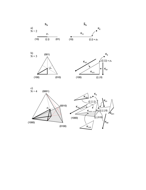
FIG. 1.: $(N-1)-$dimensional simplex ${\cal S}_{N}$ of diagonal density matrices of size $N$ and its antisymmetric part ${\widetilde{\cal S}}_{N}$ for a) $N=2$, b) $N=3$, and c) $N=4$. The simplex ${\widetilde{\cal S}}_{N}$, enlarged at the right hand side, can be decomposed into $2^{N}$ parts. $N$ numbers in brackets denote coordinates in the original $N-$dimensional space of eigenvalues. Corners of ${\widetilde{\cal S}}_{N}$ represent pure states (density matrices of rank one), edges - matrices of rank two, faces - matrices of rank two. Bold lines (grey faces) symbolise boundary of ${\widetilde{\cal S}}_{N}$.

Representation (11) makes the description of some topological properties of the $(N^{2}-1)-$dimensional space ${\cal M}$ easier [24, 25]. We introduce the following notation. We write $T^{N}=(S_{1})^{N}=[U(1)]^{N}$ for the $N-$dimensional torus. Identifying points of ${\cal S}_{N}$ which have the same coordinates (but ordered in a different way) we get an asymmetric simplex $\widetilde{\cal S}_{N}$. Equivalently, one can divide ${\cal S}_{N}$ into $N!$ identical simplexes and take any of them. The asymmetric simplex $\widetilde{\cal S}_{N}$ can be decomposed in the following natural way

$$\widetilde{\cal S}_{N}=\bigcup_{k_{1}+\dots+k_{n}=N}K_{k_{1},\dots,k_{n}}\,\text{,}$$ (12)

where $n=1,\dots,N$ denotes the number of different coordinates of a given point of $\widetilde{\cal S}_{N}$, $k_{1}$ the number of occurrences of the largest coordinate, $k_{2}$ the second largest, etc. Observe that $K_{k_{1},\dots,k_{n}}$ is homeomorphic with the set $G_{n}$, where $G_{1}$ is a single point, $G_{2}$ a half-closed interval, $G_{3}$ an open triangle with one edge but without corners, and generally, $G_{n}$ is an $(n-1)-$dimensional simplex with one $(n-2)-$dimensional hyperface without boundary (the latter is homeomorphic with an $(n-2)-$dimensional open simplex). There are $N$ ordered eigenvalues: $E_{1}\geq E_{2}\geq\cdots\geq E_{N}$, and $N-1$ independent relation operators ‘larger or equal’, which makes all together $2^{N-1}$ different possibilities. Thus, $\widetilde{\cal S}_{N}$ consists of $2^{N-1}$ parts, out of which $\binom{N-1}{m-1}$ parts are homeomorphic with $G_{m}$, when $m$ ranges from $1$ to $N$. The decomposition of the asymmetric simplex $\widetilde{\cal S}_{N}$ is illustrated in Fig. 1 for the simplest cases $N=2,3$, and $4$.

Let us denote the part of the space ${\cal M}$ related to the spectrum in $K_{k_{1},\dots,k_{n}}$ ($n$ different eigenvalues, the largest eigenvalue has $k_{1}$ multiplicity, the second largest $k_{2}$ etc.) by ${\cal M}_{k_{1},\dots,k_{n}}$. A mixed state $\rho$ with this kind of the spectrum remains invariant under arbitrary unitary rotations performed in each of the $k_{i}-$dimensional subspaces of degeneracy. Therefore the unitary matrix $B$ has a block diagonal structure with $n$ blocks of size equal to $k_{1},\dots,k_{n}$ and

$${\cal M}_{k_{1},\dots,k_{n}}\sim[U(N)/(U(k_{1})\times\cdots\times U(k_{n}))]\times G_{n}\,\text{,}$$ (13)

where $k_{1}+\dots+k_{n}=N$ and $k_{i}>0$ for $i=1,\dots,n$. Thus $\cal M$ has the structure

$${\cal M}\sim\bigcup_{k_{1}+\dots+k_{n}=N}{\cal M}_{k_{1},\dots,k_{n}}\sim\bigcup_{k_{1}+\dots+k_{n}=N}[U(N)/(U(k_{1})\times\cdots\times U(k_{n}))]\times G_{n}\,\text{,}$$ (14)

where the sum ranges over all partitions of $N$. The group of rotation matrices $B$ equivalent to $\Gamma=U(k_{1})\times U(k_{2})\times\cdots\times U(k_{n})$ is called the stability group of $U(N)$.

For $N=2$ we have ${\cal M}_{1,1}\sim[U(2)/T^{2}]\times G_{2}\sim S^{2}\times G_{2}$ and ${\cal M}_{2}\sim\{\rho_{*}\}$, so the space ${\cal M}$ has the topology of a two-dimensional ball - the Bloch sphere and its interior. This case and also cases $N=3,4$ are analysed in detail in Tab. 1.

$N$	Label	Decomposition	Subspace	Part of the asymmetric simplex	Topological Structure	Dimension $D=D_{1}+D_{2}$
$1$	${\cal M}_{1}$	$1$	$E_{1}$	point	$[U(1)/U(1)]\times G_{1}=\{\rho_{\ast}\}$	$0=0+0$
$2$	${\cal M}_{11}$	$1+1$	$E_{1}>E_{2}$	line with left edge	$[U(2)/T^{2}]\times G_{2}$	$3=2+1$
	${\cal M}_{2}$	$2$	$E_{1}=E_{2}$	right edge	$[U(2)/U(2)]\times G_{1}=\{\rho_{\ast}\}$	$0=0+0$
	${\cal M}_{111}$	$1+1+1$	$E_{1}>E_{2}>E_{3}$	triangle with base without corners	$[U(3)/T^{3}]\times G_{3}$	$8=6+2$
$3$	${\cal M}_{12}$	$1+2$	$E_{1}>E_{2}=E_{3}$	edges with	$[U(3)/(U(2)\times T)]\times G_{2}$	$5=4+1$
	${\cal M}_{21}$	$2+1$	$E_{1}=E_{2}>E_{3}$	lower corners
	${\cal M}_{3}$	$3$	$E_{1}=E_{2}=E_{3}$	upper corner	$[U(3)/U(3)]\times G_{1}=\{\rho_{\ast}\}$	$0=0+0$
	${\cal M}_{1111}$	$1+1+1+1$	$E_{1}>E_{2}>E_{3}>E_{4}$	interior of tetrahedron with bottom face	$[U(4)/T^{4}]\times G_{4}$	$15=12+3$
	${\cal M}_{112}$	$1+1+2$	$E_{1}>E_{2}>E_{3}=E_{4}$
	${\cal M}_{121}$	$1+2+1$	$E_{1}>E_{2}=E_{3}>E_{4}$	faces without side edges	$[U(4)/(U(2)\times T^{2})]\times G_{3}$	$12=10+2$
$4$	${\cal M}_{211}$	$2+1+1$	$E_{1}=E_{2}>E_{3}>E_{4}$
	${\cal M}_{13}$	$1+3$	$E_{1}>E_{2}=E_{3}=E_{4}$		$[U(4)/(U(3)\times T)]\times G_{2}$	$7=6+1$
	${\cal M}_{31}$	$3+1$	$E_{1}=E_{2}=E_{3}>E_{4}$	edges with lower corners
	${\cal M}_{22}$	$2+2$	$E_{1}=E_{2}>E_{3}=E_{4}$		$[U(4)/(U(2)\times U(2))]\times G_{2}$	$9=8+1$
	${\cal M}_{4}$	$4$	$E_{1}=E_{2}=E_{3}=E_{4}$	upper corner	$[U(4)/U(4)]\times G_{1}=\{\rho_{\ast}\}$	$0=0+0$

Table 1.  Topological structure of the space of mixed quantum states for a fixed number of levels $N$. The group of unitary matrices of size $N$ is denoted by $U(N)$, the unit circle (one-dimensional torus $\sim U(1)$) by $T$, while $G_{n}$ stands for a part of an $(n-1)-$dimensional asymmetric simplex defined in the text. Dimension $D$ of the component ${\cal M}_{k_{1},\dots,k_{n}}$ equals $D_{1}+D_{2}$, where $D_{1}$ denotes the dimension of the quotient space $U(N)/\Gamma$, while $D_{2}=n-1$ is the dimension of the part of the eigenvalues simplex homeomorphic with $G_{n}$.

Note that the part $M_{1,\dots,1}$ represents generic, non-degenerate spectrum. In this case all elements of the spectrum of $\rho$ are different and the stability group $H$ is equivalent to an $N$-torus

$${\cal M}_{1,\ldots,1}\sim[U(N)/T^{N}]\times G_{N}\,\text{.}$$ (15)

Above representation of generic states enables us to define a product measure in the space ${\cal M}$ of mixed quantum states. For this end, one can take the uniform (Haar) measure on $U(N)$ and a certain measure on the simplex ${\cal S}_{N}$ [26, 27]. The coordinates of a point on the simplex may be generated [28] by squared moduli of components of a random orthogonal (unitary) matrix [29].

The other $2^{N-1}-1$ parts of $\cal M$ represent various kinds of degeneracy and have measure zero. The number of non-homeomorphic parts is equal to the number $P(N)$ of different representations of the number $N$ as the sum of positive natural numbers. Thus $P(N)$ gives the number of different topological structures present in the space $\cal M$. For $N=1,2,\dots,10$ the number $P(N)$ is equal to $1,2,3,5,7,11,15,22,30$ and $42$, while for larger $N$ there is described by the asymptotic Hardy-Ramanujan formula [30], $P(N)\sim\exp\left(\pi\sqrt{2N/3}\right)/4\sqrt{3}N$.

In the extreme case of $N$-fold degeneracy, $E_{i}\equiv 1/N$, the subspace ${\cal M}_{N}\sim[U(N)/(U(N)\times T^{0})]\times G_{1}\sim G_{1}$, so it degenerates to a single point. This distinguishes the maximally mixed state $\rho_{\ast}:={\bf I}/N$, which will play a crucial role in subsequent considerations. For the manifold of pure states $n=2$ and $k_{1}=1,k_{2}=N-1$ (since $E_{1}=1$, $E_{2}=\cdots=E_{N}=0$) and so ${\cal P}\sim[U(N)/(U(N-1)\times U(1))]\times(1,0,\dots,0)\sim{\mathbb{C}}P^{N-1}$. In the case $N=2$ it can be identified with the Bloch sphere $S^{2}$.

On the other hand, it is well known that $\cal M$ itself has a structure of a simplex with the boundary contained in the hypersurface det$\rho=0$, with rank 1 matrices (pure states - $\cal P$) as ‘corners’, rank 2 as ‘edges’, etc., and with the point $\rho_{\ast}$ ‘in the middle’ (see [31, 32] for a formal statement and [33] for a nice intuitive discussion).

Let us mention in passing that the quotient space appearing in (13)

$${\mathbb{F}}:={U(N)\over U(k_{1})\times U(k_{2})\times\cdots\times U(k_{n})}$$ (16)

is called a flag manifold, and in a special case

$$Gr(k,N):={U(N)\over U(k)\times U(N-k)}$$ (17)

a Grassman manifold. For a fuller discussion of the topological structure of $\cal M$ (especially for $N=4$) we refer the reader to [24].

B Metric properties

The density matrix of a pure state $\rho_{\psi}=|\psi\rangle\langle\psi|$ may be represented in a suitable basis by a matrix with the first element equal to unity and all others equal to zero. Due to this simple form it is straightforward to compute the standard distances between $\rho_{\psi}$ and $\rho_{*}$ directly from the definitions recalled in Sect. 1. Results do depend on the dimension $N$, but are independent on the pure state $|\psi\rangle$, namely

$$D_{tr}(\rho_{\psi},\rho_{*})=2-\frac{2}{N}\,,\qquad D_{HS}(\rho_{\psi},\rho_{*})=\sqrt{1-\frac{1}{N}}\,,\qquad D_{Bures}(\rho_{\psi},\rho_{*})=\sqrt{2-\frac{2}{\sqrt{N}}}\,\text{.}$$ (18)

In the sense of the trace, the Hilbert-Schmidt, or the Bures metric the $2(N-1)-$dimensional space of pure states ${\cal P}$ may be therefore considered as a part of the $(N^{2}-1)-$dimensional sphere centred at $\rho_{*}$ of the radius $r$ depending on $N$ and on the metric used. From the point of view of these standard metrics, no pure state on ${\cal P}$ is distinguished; all of them are equivalent. It is easy to show that the distance of any mixed state from $\rho_{*}$ is smaller than $r$, in the sense of each of the standard metrics. Thus the space of mixed states ${\cal M}$ lays inside the sphere $S^{N^{2}-2}$ embedded in ${\mathbb{R}}^{N^{2}-1}$, although, as discussed above, its topology (for $N>2$) is much more complicated than the topology of the $(N^{2}-1)-$dimensional disk.

The degree of mixture of any state may be measured, e.g., by the von Neumann entropy $S=-{\rm Tr}\rho\ln\rho=-\sum_{i=1}^{N}E_{i}\ln(E_{i})$. It varies from zero (pure states) to ln($N$) (the maximally mixed state $\rho_{*}$). Let us briefly discuss a simple kicked dynamics, generated by a Hamiltonian represented by a Hermitian matrix $H$ of size $N$. It maps a state $\rho$ into

$$\rho^{\prime}=e^{iH}\rho e^{-iH}\,\text{,}$$ (19)

where the kicking period is set to unity.

Such a unitary quantum map does not change the eigenvalues of $\rho$, so the von Neumann entropy is conserved. In particular, any pure state is mapped by (19) into a pure state. Any mixed state $\rho$, which commutes with $H$, is not affected by this dynamics. Assume the Hamiltionian $H$ to be generic, in the sense that its $N$ eigenvalues are different. Then its invariant states form an $(N-1)-$dimensional subspace ${\cal{I}}_{H}\subset M$, topologically equivalent to ${\cal S}_{N}$. In the generic case of non-degenerate Hamiltonian it contains only $N$ pure states: the eigenstates of $H$. Note that the invariant subspace ${\cal I}_{H}$ always contains $\rho_{\ast}$.

Moreover, the standard distances between two states are conserved under the action of a unitary dynamics, i.e.

$$D_{s}(\rho_{1},\rho_{2})=D_{s}(\rho_{1}^{\prime},\rho_{2}^{\prime})\,\text{,}$$ (20)

where $D_{s}$ denotes one of the distances: $D_{tr}$, $D_{HS}$ or $D_{Bures}$. Therefore, the unitary dynamics given by (19) can be considered as a generalised rotation in the $(N^{2}-1)-$dimensional space ${\cal M}$, around the $(N-1)-$dimensional ‘hyperaxis’ ${\cal I}_{H}$, which is topologically equivalent to the simplex $S^{N-1}$. In the simplest case, $N=2$, it is just a standard rotation of the Bloch ball around the axis determined by $H$. For example, if $H=\alpha J_{z}$, where $J_{z}$ is the third component of the angular momentum operator $J$, it is just the rotation by angle $\alpha$ around the $z$ axis joining both poles of the Bloch sphere. The set ${\cal I}_{H}$ of states invariant with respect to this dynamics consists of all states diagonal in the basis of $J_{z}$: the mixed states with diag$(\rho)=\{a,1-a\}$ ($a\in(0,1)$) and two pure states, $|1/2,1/2\rangle$ for $a=1$, and $|1/2,-1/2\rangle$ for $a=0$.

III Monge distance between quantum states

A Monge transport problem and the Monge-Kantorovich distance

The original Monge problem, formulated in 1781 [34], emerged from studying the most efficient way of transporting soil [35]:

Split two equally large volumes into infinitely small particles and then associate them with each other so that the sum of products of these paths of the particles over the volume is least. Along which paths must the particles be transported and what is the smallest transportation cost?

Consider two probability densities $Q_{1}$ and $Q_{2}$ defined in an open set $\Omega\subset R^{n}$, i.e., $Q_{i}\geq 0$ and $\int_{\Omega}Q_{i}(x)d^{n}x=1$ for $i=1,2$. Let $V_{1}$ and $V_{2}$, determined by $Q_{i}$, describe the initial and the final location of ‘soil’: $V_{i}=\{\left(x,y\right)\in\Omega\times R^{+}:0\leq y\leq Q_{i}(x)\}$. The integral $\int_{V_{i}}d^{n}x\,dy$ is equal to the unity due to normalisation of $Q_{i}$. Consider $C^{1}$ one-to-one maps $T:\Omega\to\Omega$ which generate volume preserving transformations $V_{1}$ into $V_{2}$, i.e.,

$$Q_{1}\left(x\right)=Q_{2}\left(Tx\right)\left|T^{\prime}(x)\right|$$ (21)

for all $x\in\Omega$, where $T^{\prime}(x)$ denotes the Jacobian of the map $T$ at point $x$. We shall look for a transformation giving the minimal displacement integral and define the Monge distance [35, 36]

$$D_{M}(Q_{1},Q_{2}):={\inf}\int_{\Omega}|x-T(x)|Q_{1}\left(x\right)d^{n}x\,\text{,}$$ (22)

where the infimum is taken over all $T$ as above. If the optimal transformation $T_{M}$ exists, it is called a Monge plan. Note that in this formulation of the problem the ‘vertical’ component of the soil movement is neglected. The problem of existence of such a transformation was solved by Sudakov [37], who proved that a Monge plan exists for $Q_{1},Q_{2}$ smooth enough (see also [38]). The above definition can be extended to an arbitrary metric space $(\Omega,d)$ endowed with a Borel measure $m$. In this case one should put $d(x,T(x))$ instead of $|x-T(x)|$ and $dm(x)$ instead of $d^{n}x$ in formula (22), and take the infimum over all one-to-one and continuous $T:\Omega\to\Omega$ fulfilling $\int_{A}Q_{1}dm=\int_{T^{-1}(A)}Q_{2}dm$ for each Borel set $A\subset\Omega$. In fact we can also measure the Monge distance between arbitrary two probability measures in a metric space $(\Omega,d)$. For $\mu,\nu$ - probability measures on $(\Omega,d)$ we put

$$D_{M}(\mu,\nu):={\inf}\int_{\Omega}d(x,T(x))d\mu(x)\ \text{,}$$ (23)

where the infimum is taken over all one-to-one and continuous $T:\Omega\to\Omega$ such that $\mu(A)=\nu(T^{-1}(A))$ for each Borel set $A\subset\Omega$. To avoid the problem of the existence of a Monge plan Kantorovich [39, 40] introduced in 40s the ‘weak’ version of the original Monge’s mass allocation problem and proved his famous variational principle (see Proposition 1). For this and other interesting generalisations of the Monge problem consult the monographs by Rachev and Rüschendorf [36, 41].

In some cases one can find the Monge distance analytically. For the one-dimensional case, $\Omega=\mathbb{R}$, the Monge distance can be expressed explicitly with the help of distribution functions $F_{i}(x)=\int_{-\infty}^{x}Q_{i}(t)dt$, $i=1,2$. Salvemini obtained the following solution of the problem [43]

$$D_{M}(Q_{1},Q_{2})=\int_{-\infty}^{+\infty}|F_{1}(x)-F_{2}(x)|dx\,\text{.}$$ (24)

Several two-dimensional problems with some kind of symmetry can be reduced to one-dimensional problems, solved by (24). In the general case one can estimate the Monge distance numerically [44], relying on algorithms of solving the transport problem, often discussed in handbooks of linear programming [45].

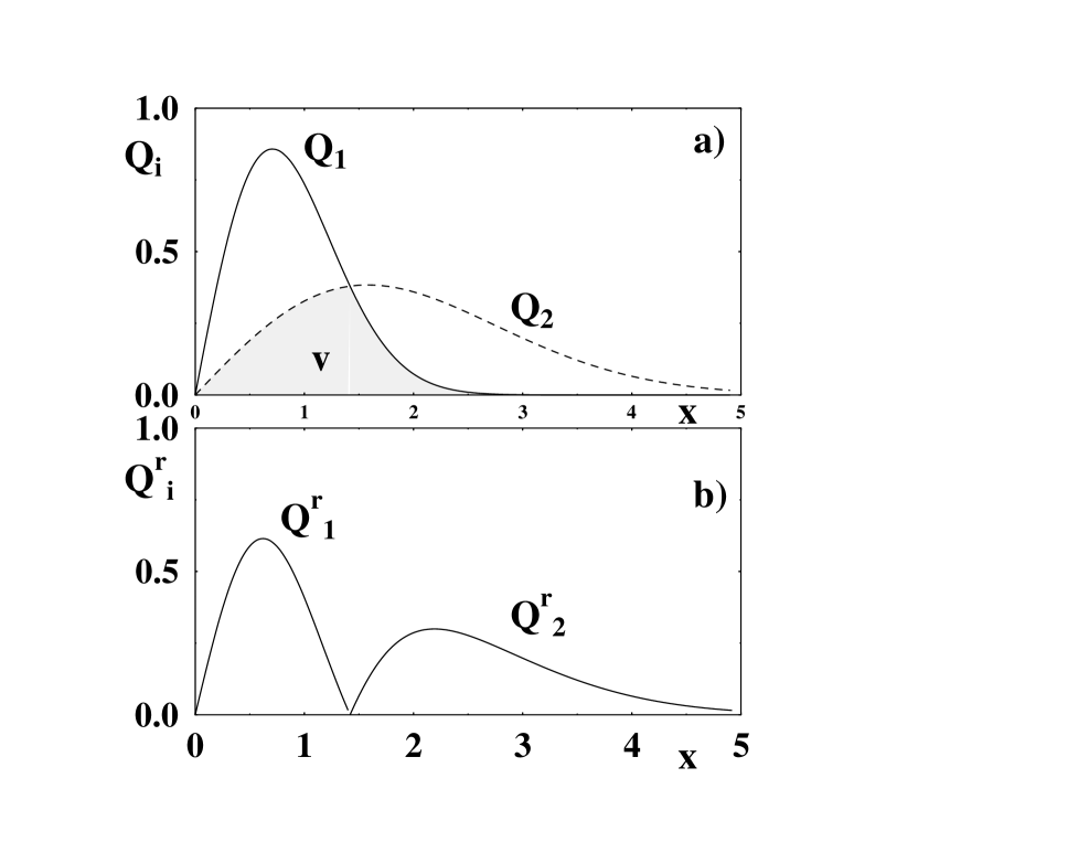
FIG. 2.: Estimation of the Monge distance between two overlapping distributions $Q_{1}$ and $Q_{2}$ (a) by the distance between the reduced distributions ${Q}^{r}_{i}(x)=Q_{i}(x)-V(x)$ (b), where $V(x)$ denotes the overlap.

According to definition (22) taking an arbitrary map $T$ which fulfils (21) we obtain an upper bound for the Monge distance $D_{M}$. Another two methods of estimating the Monge distance are valid for a compact metric space $(\Omega,d)$ equipped with a finite measure $m$. The first method may be used to obtain lower bounds for $D_{M}$. It is based on the proposition proved by Kantorovich in 40s [39, 40] (see also [36, 41, 38]).

Proposition 1. (variational formula for the Monge-Kantorovich metric)

$$D_{M}(Q_{1},Q_{2})=\max\left|\int_{\Omega}f(x)(Q_{1}(x)-Q_{2}(x))dm(x)\thinspace\right|\,\text{,}$$ (25)

where the supremum is taken over all $f$ fulfilling the condition $|f(x)-f(y)|\leq d(x,y)$ for all $x,y\in\Omega$ (weak contractions).

To obtain another upper bound for $D_{M}$ we may apply the following simple estimate:

Proposition 2.

$$D_{M}(Q_{1},Q_{2})\leq(\Delta/2)D_{L_{1}}(Q_{1},Q_{2}),$$ (26)

where $D_{L_{1}}(Q_{1},Q_{2})=\int_{\Omega}|Q_{1}(x)-Q_{2}(x)|dm(x)$ and $\Delta=\operatorname*{diam}(\Omega)$.

The intuitive explanation of this fact is the following. Let $v$ be the volume of the ‘overlap’ of the probability distributions $Q_{1}$ and $Q_{2}$, i.e., $v=\int_{\Omega}V(x)dm(x)$, where $V=\min\{Q_{1},Q_{2}\}$. Then $D_{M}(Q_{1},Q_{2})\leq(1-v)\Delta$, because the number $(1-v)$ represents the part of the distribution to be moved and the largest possible classical distance on $\Omega$ is smaller than or equal to $\Delta$. Moreover, $D_{L_{1}}(Q_{1},Q_{2})=2(1-v)$, which proves the assertion. Although Fig. 2 presents the corresponding picture for the simplest, one-dimensional case, Proposition 2 is valid for an arbitrary metric space. For the formal proof see Appendix A.

B The Monge distance - harmonic oscillator coherent states

In [20] we defined a ‘classical’ distance between two quantum states $\rho_{1}$ and $\rho_{2}$ via the Monge distance between the corresponding Husimi distributions $H_{\rho_{1}}$ and $H_{\rho_{2}}$:

$$D_{M}(\rho_{1},\rho_{2}):=D_{M}\left({H_{\rho_{1}},H_{\rho_{2}}}\right)\,\text{,}$$ (27)

where $H_{\rho_{i}}$ are given by formula (9). Observe that the family of harmonic oscillator coherent states $|\alpha\rangle$, parameterised by a complex number $\alpha$, is implicitly present in this definition.

The Monge distance satisfies the semiclassical property: the distance between any two Glauber coherent states, represented by Gaussian Husimi distributions localised at points $a_{1}$ and $a_{2}$, is equal to the classical distance $|a_{1}-a_{2}|$ in the complex plane [20].

C The Monge distance - general case and basic properties

The above construction, originally performed for the complex plane with the help of the harmonic oscillator coherent states, may be extended to arbitrary generalised coherent states of Perelomov [46] defined on a compact classical phase space. Let $G$ be a compact Lie group, $G\ni g\to R_{g}\in{\cal H}$ its irreducible unitary representation in the Hilbert space $\cal H$, and $\Upsilon$ the subgroup of $G$, which consists of all elements $y\in G$ leaving the reference state $|\kappa\rangle\in{\cal P}$ invariant (i.e. $R_{y}|\kappa\rangle\sim|\kappa\rangle$). Define $\Omega=G/\Upsilon$ and $|\eta\rangle=R_{\eta}|\kappa\rangle$ for $[\eta]\in G/\Upsilon$. Note that $|1\rangle=|\kappa\rangle$, where $1$ is the group $G$ unit. Consider a family of the generalised coherent states $\Omega\ni\eta\to|\eta\rangle\in{\cal P}$. It satisfies the identity resolution $\int_{\Omega}|\eta\rangle\langle\eta|dm(\eta)={\bf I}/\dim\cal{H}$, where $m$ is the natural (translation invariant) measure on the Riemannian manifold $(\Omega,d)$ normalised by the condition $m(\Omega)=1$, and $d$ is the Riemannian metric on $\Omega$. Let us denote by ${\cal C}$ the manifold of all quantum coherent states, isomorphic to $\Omega$, and embedded in the space of all pure states ${\cal P}$. Note that $\langle\eta|\eta\rangle\equiv 1$.

For the $SU(k)$ coherent states the space $\Omega\sim{\cal C}$ is isomorphic to ${\mathbb{C}}P^{k-1}$ and $m$ is the natural Riemannian measure on $\Omega$. Obviously, the dimension of the Hilbert space ${\cal H}_{N}$ carrying the representation of the group equals $N\geq k$, and if $N=k$ all pure states are $SU(k)$ coherent, and ${\cal C}={\cal P}$. For example, in the case of $SU(2)$ vector coherent states the corresponding classical phase space is the sphere $S^{2}\simeq{\mathbb{C}}P^{1}$ [46]. In the simplest case $N=2$ (or $j=1/2$) pure states are located at the Bloch sphere and are coherent.

Any quantum state $\rho\in\cal{M}$ may be represented by a generalised Husimi distribution $H_{\rho}:\Omega\to\mathbb{R}^{+}$ defined by

$$H_{\rho}(\eta):=N\cdot\langle\eta|\rho|\eta\rangle\,\text{,}$$ (28)

for $\eta\in\Omega$, which satisfies

$$\int_{\Omega}H_{\rho}(\eta)dm(\eta)=1\,\text{.}$$ (29)

In particular, for a pure state $\rho=|\vartheta\rangle\langle\vartheta|$ ($|\vartheta\rangle\in\cal{P}$) and $\eta\in\Omega$ we have

$$H_{|\vartheta\rangle\langle\vartheta|}(\eta):=N{|\langle\vartheta|\eta\rangle|}^{2}\,\text{.}$$ (30)

In the sequel we shall assume that for coherent states $|\vartheta\rangle\in\cal{C}$ ($\vartheta\in\Omega$) the densities $H_{|\vartheta\rangle\langle\vartheta|}$ tend weakly to the Dirac-delta measure $\delta_{\vartheta}$ in the semiclassical limit, i.e., when the dimension of the Hilbert space carrying the representation tends to infinity.

The Monge distance for the Hilbert space ${\cal H}_{N}$, the classical phase space $(\Omega,d)$ and the corresponding family of generalised coherent states $|\eta\rangle$ is then defined by solving the Monge problem in $\Omega$, in the full analogy with (27):

$$D_{M}(\rho_{1},\rho_{2}):=D_{M}\left({H_{\rho_{1}},H_{\rho_{2}}}\right)\,\text{.}$$ (31)

The distance $d(\eta,T(\eta))$ between the initial point $\eta$ and its image $T(\eta)$ with respect to the Monge plan has to be computed along the geodesic lines on the Riemannian manifold $\Omega$.

For compact spaces $\Omega$ the semiclassical condition (8) for the distance between two coherent states becomes weaker:

Property A. (semiclassical condition) Let $\eta_{1},\eta_{2}\in\Omega$. Then

$$D_{M}(|\eta_{1}\rangle,|\eta_{2}\rangle)\leq d(\eta_{1},\eta_{2})\,\text{,}$$ (32)

and

$$D_{M}(|\eta_{1}\rangle,|\eta_{2}\rangle)\to d(\eta_{1},\eta_{2})\qquad\text{(in the semiclassical limit)}\text{,}$$ (33)

where $d$ represents the Riemannian distance between two points in $\Omega$.

To demonstrate (32) it suffices to take for the transformation $T$ in (22) the group translation ${\eta_{2}}*{\eta_{1}}^{-1}$ (e.g. the respective rotation of the sphere $S^{2}$ in the case of $SU(2)$ coherent states). However, this transformation needs not to give the optimal Monge plan. As we shall show in the following section, this is so for the sphere and the $SU(2)$ coherent states. On the other hand, in the semiclassical limit (for $SU(2)$ coherent states: $j\to\infty$), the inequality in (32) converts into the equality, in the full analogy to the property (8), valid for the complex plane and the harmonic oscillator coherent states. This follows from the fact that the Monge- Kantorovich metric generates the weak topology in the space of all probability measures on $\Omega$, and the densities $H_{|\eta_{i}\rangle\langle\eta_{i}|}$ tend weakly to the Dirac-delta $\delta_{\eta_{i}}$ in the semiclassical limit, for $i=1,2$.

The Monge distance defined above is invariant under the action of group translations, namely:

Property B. (invariance) Let $\alpha,\beta\in G$ and $\rho_{1},\rho_{2}\in\cal{M}$. Then

$$D_{M}({R_{\beta}}^{-1}\rho_{1}R_{\beta},{R_{\beta}}^{-1}\rho_{2}R_{\beta})=D_{M}(\rho_{1},\rho_{2})\,\text{.}$$ (34)

Particularly,

$$D_{M}(|\alpha\rangle,|\beta\rangle)=D_{M}(|{\beta}^{-1}\alpha\rangle,|1\rangle)\,\text{,}$$ (35)

where $1$ is the group $G$ unit.

The above formulae follow from the definition of the Monge distance (23), and from the fact that both the measure $m$ and the metric $d$ are translation invariant.

D Relation to other distances

Let $\rho_{1},\rho_{2}\in\cal{M}$. We start from recalling the variational formula for the trace distance (see for instance [47]).

Proposition 3. (variational formula for $D_{tr}$)

$$D_{tr}(\rho_{1},\rho_{2})=\sup_{\left\|{A}\right\|\leq 1}|\operatorname*{tr}A(\rho_{1}-\rho_{2})|\,\text{,}$$ (36)

where the supremum is taken over all Hermitian matrices $A$ such that $\left\|{A}\right\|\leq 1$, and the supremum norm reads

$$\left\|{A}\right\|=\sup\{\left\|{Ax}\right\|:x\in{\cal{H}_{N}},\left\|{x}\right\|\leq 1\}\,\text{.}$$ (37)

Applying Proposition 1 we can prove an analogous formula for the Monge distance

Proposition 4. (variational formula for $D_{M}$)

$$D_{M}(\rho_{1},\rho_{2})=\max_{L(A)\leq 1}|\operatorname*{tr}A(\rho_{1}-\rho_{2})|\,\text{,}$$ (38)

where the maximum is taken over all Hermitian matrices $A$ with $L(A)\leq 1$, and

$$L(A)=\inf\{c:\text{there exists a {\hbox{c}}-Lipschitzian function}\ f:\Omega\rightarrow{\mathbb{R}}\ \text{such that}\ A=\int_{\Omega}f(\eta)|\eta\rangle\langle\eta|dm(\eta)\}\,\text{.}$$ (39)

For the proof see Appendix B. This proposition has a simple physical interpretation. It says that the Monge distance between two quantum states is equal to the maximal value of the difference between the expectation values (in these states) of observables (Hermitian operators) some of whose P-representations are weak contractions. Recently, Rieffel [48] considered the class of metrics on state spaces which are generated by Lipschitz seminorms. If $\Omega$ is compact, then one can show that the Monge metric $D_{M}$ belongs to this class.

From Propositions 3 and 4 we can also easily deduce Proposition 2. Using Proposition 2 and the Hölder inequality for the trace (see [47]) one can prove the following inequalities

$${2\over\Delta}D_{M}\leq D_{L_{1}}\leq N\cdot D_{HS}\leq N\cdot D_{tr}\,\text{,}$$ (40)

where $\Delta$ is the diameter of $\Omega$ and $N=\dim\cal{H}_{N}$. On the other hand from the fact that the Monge-Kantorovich metric generates the weak topology in the space of probability measures on $\Omega$, it follows that $D_{M}(\rho_{1},\rho_{2})\to 0$ implies $D_{HS}(\rho_{1},\rho_{2})\to 0$ for every $\rho_{1},\rho_{2}\in\cal{M}$. Thus the Monge metric $D_{M}$ and the Hilbert-Schmidt metric $D_{HS}$ generate the same topology in the space of mixed states $\cal{M}$.

Let us emphasise here a crucial difference between our ‘classical’ Monge distance and the standard distances in the space of quantum states. Given any two quantum states represented by the density matrices $\rho_{1}$ and $\rho_{2}$, one may directly compute the trace, the Hilbert-Schmidt or the Bures distance between them. On the other hand, the classical distance is defined by specifying the set of generalised coherent states in the Hilbert space. In other words, one needs to choose a classical phase space with respect to which the Monge distance is defined. Take for example two density operators of size $N=3$. The distance $D_{M}(\rho_{1},\rho_{2})$ computed with respect to the $SU(2)$ coherent states and, say, with respect to the $SU(3)$ coherent states can be different. The simplest case of the $SU(2)$ coherent states corresponding to classical dynamics on the sphere is discussed in the following section.

IV Monge metric on the sphere

A Spin coherent states representation

Let us consider a classical area preserving map on the sphere $\Theta:S^{2}\to S^{2}$ and a corresponding quantum map $U$ acting in an $N-$dimensional Hilbert space ${\cal H}_{N}$. A link between classical and quantum mechanics can be established via a family of spin coherent states $|\vartheta,\varphi\rangle\in{\cal H}$ localised at points $(\vartheta,\varphi)$ of the sphere ${\mathbb{C}}P^{1}=S^{2}$. The vector coherent states were introduced by Radcliffe [49] and Arecchi et al. [50] and their various properties are often analysed in the literature (see e.g. [51, 52]). They are related to the $SU(2)$ algebra of the components of the angular momentum operator $J=\{J_{x},J_{y},J_{z}\}$, and provide an example of the general group theoretic construction of Perelomov [46] (see Sect. III C).

Let us choose a reference state $|\kappa\rangle$, usually taken as the maximal eigenstate $|j,j\rangle$ of the component $J_{z}$ acting on ${\cal H}_{N}$, $N=2j+1$, $j=1/2,1,3/2,\dots$. This state, pointing toward the ‘north pole’ of the sphere, enjoys the minimal uncertainty equal to $j$. Then, the vector coherent state is defined by the Wigner rotation matrix $R_{\vartheta,\varphi}$

$$|\vartheta,\varphi\rangle=\thinspace R_{\vartheta,\varphi}|\kappa\rangle=\thinspace(1+|\gamma|^{2})^{-j}e^{\gamma J_{-}}|j,j\rangle\,\text{,}$$ (41)

where $R_{\vartheta,\varphi}=\exp\left[{i\vartheta\left({\cos\varphi J_{x}-\sin\varphi J_{y}}\right)}\right]$, $J_{-}=J_{x}-iJ_{y}$ and $\gamma={\tan}(\vartheta/2)e^{i\varphi}$, for $(\vartheta,\varphi)\in S^{2}$ (we use the spherical coordinates).

We obtain the coherent states identity resolution in the form

$$\int_{S^{2}}|\vartheta,\varphi\rangle\langle\vartheta,\varphi|\ d\mu(\vartheta,\varphi)={\bf I}/(2j+1)\,\text{,}$$ (42)

where the Riemannian measure $d\mu(\vartheta,\varphi)=(\sin\vartheta/4\pi)d\vartheta d\varphi$ does not depend on the quantum number $j$.

Expansion of a coherent state in the common eigenbasis of $J_{z}$ and $J^{2}$: $|j,m\rangle$, $m=-j,\dots,+j$ (in ${\cal H}_{N}$) reads

$$|\vartheta,\varphi\rangle=\sum_{m=-j}^{m=j}\sin^{j-m}(\vartheta/2)\cos^{j+m}(\vartheta/2)\exp\left({i(j-m)\varphi}\right)\left[\binom{2j}{j-m}\right]^{1/2}|j,m\rangle\,\text{.}$$ (43)

The infinite ‘basis’ formed in the Hilbert space by the coherent states is overcomplete. Two different $SU(2)$ coherent states overlap unless they are directed into two antipodal points on the sphere. Expanding the coherent states in the basis of ${\cal H}_{N}$ as in (43) we calculate their overlap

$${|\langle\vartheta^{\prime},\varphi^{\prime}|\vartheta,\varphi\rangle|^{2}}=\cos^{4j}(\Xi/2)\,\text{,}$$ (44)

where $\Xi$ is the angle between two vectors on $S^{2}$ related to the coherent states $|\vartheta,\varphi\rangle$ and $|\vartheta^{\prime},\varphi^{\prime}\rangle$, and for $j=1/2$ it equals to the geodesic distance (7). Thus, we have

$$H_{|\vartheta,\varphi\rangle\langle\vartheta,\varphi|}(\vartheta^{\prime},\varphi^{\prime})=(2j+1)\cos^{4j}(\Xi/2)\,\text{.}$$ (45)

This formula guarantees that the respective Husimi distribution of an arbitrary spin coherent state tends to the Dirac $\delta$–function in the semiclassical limit $j\to\infty$.

To calculate the Monge distance between two arbitrary density matrices $\rho_{1}$ and $\rho_{2}$ of size $N$ one uses the $N=(2j+1)-$dimensional representation of the spin coherent states $|\vartheta,\varphi\rangle$ (to simplify the notation we did not label them by the quantum number $j$). Next, one computes the generalised Husimi representations for both states

$$H_{\rho_{i}}(\vartheta,\varphi):=N\cdot\langle\vartheta,\varphi|\rho_{i}|\vartheta,\varphi\rangle$$ (46)

and solves the Monge problem on the sphere for these distributions. Increasing the parameter $j$ (quantum number) one may analyse the semiclassical properties of the Monge distance.

It is sometime useful to use the stereographical projection of the sphere $S^{2}$ onto the complex plane. The Husimi representation of any state $\rho$ becomes then the function of a complex parameter $z$. It is easy to see that for any pure state $|\psi\rangle\in{\cal P}$ the corresponding Husimi representation is given by a polynomial of $(N-1)$ order: $W_{\psi}(z)=z^{N-1}+\sum_{i=0}^{N-2}c_{l}z^{l}=0$ with arbitrary complex coefficients $c_{i}$. This fact provides an alternative explanation of the equality ${\cal P}={\mathbb{C}}P^{N-1}$. Thus, every pure state can be uniquely determined by the position of the $(N-1)$ zeros of $W_{\psi}$ on the complex plane (or, equivalently, by zeros of $H_{|\psi\rangle}$ on the sphere). Such stellar representation of pure states is due to Majorana [53] and it found several applications in the investigation of quantum dynamics [54, 55, 56]. In general, the zeros of Husimi representation may be degenerated. This is just the case for the coherent states: the Husimi function of the state $|\vartheta,\varphi\rangle$ is equal to zero only at the antipodal point and the $(N-1)-$fold degeneracy occurs. The stellar representation is used in section VI to define a simplified Monge metric in the space of pure quantum states.

B Monge distance between some symmetrical states

Consider two quantum states, whose Husimi distributions are invariant with respect to the horizontal rotation. Using Proposition 4 one may found the Monge distance between both states with the help of the Salvemini formula (24)

Proposition 5. Let $\rho_{1},\rho_{2}\in\cal{M}$  fulfil  ${H}_{\rho_{i}}(\vartheta,\varphi)={\tilde{H}}_{\rho_{i}}(\vartheta)$  for $(\vartheta,\varphi)\in S^{2}$. Consider the normalised one-dimensional functions $h_{\rho_{i}}:[0,\pi]\to\mathbb{R}^{+}$ given by $h_{\rho_{i}}(\vartheta):={\tilde{H}}_{\rho_{i}}(\vartheta)\frac{1}{2}\sin\vartheta$, that satisfy $\int_{0}^{\pi}h_{\rho_{i}}(\vartheta)d\vartheta=1$ for $i=1,2$. Then

$$D_{M}(\rho_{1},\rho_{2})=\int_{0}^{\pi}\left|F_{\rho_{1}}(\vartheta)-F_{\rho_{2}}(\vartheta)\right|d\vartheta\,\text{,}$$ (47)

where the cumulative distributions read $F_{\rho_{i}}(\vartheta)=\int_{0}^{\vartheta}h_{\rho_{i}}(\psi)d\psi$.

The proof is given in Appendix C. We use this proposition computing the Monge distance between two arbitrary eigenstates of the operator $J_{z}$ (Sect. IV F1) and the Monge distance of some of these eigenstates from the maximally mixed state (Sect. IV F2).

The maximally mixed state $\rho_{\ast}={\bf I}/N$ is represented by the uniform Husimi distribution on the sphere. Thus, ${H}_{\rho_{\ast}}(\vartheta,\varphi)={\tilde{H}}_{\rho_{\ast}}(\vartheta)=1$, $h_{\rho_{\ast}}(\vartheta)=\frac{1}{2}\sin\vartheta$, and $F_{\rho_{\ast}}(\vartheta)=\frac{1}{2}(1-\cos\vartheta)$.

Furthermore, all the eigenstates of $J_{z}$, forming the basis $|j,m\rangle$, possess this symmetry, and according to (43) we get

$$h_{|j,m\rangle\langle j,m|}(\vartheta)=(2j+1)\binom{2j}{j-m}\sin^{2(j-m)+1}(\vartheta/2)\cos^{2(j+m)+1}(\vartheta/2)\,\text{.}$$ (48)

The formula (47) enables us to compute the Monge distance between them.

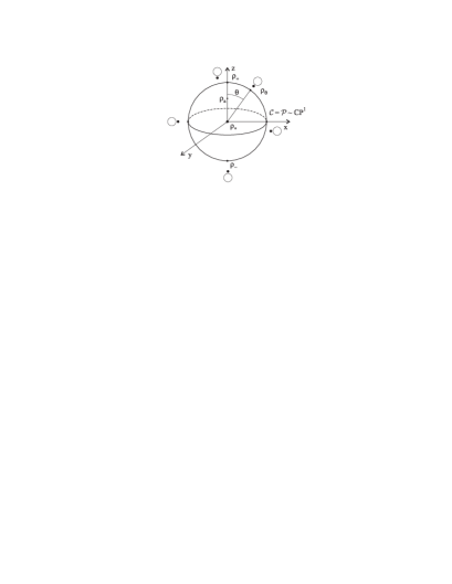
FIG. 3.: Quantum states, for which we calculate Monge distances, are denoted at the Bloch sphere corresponding to $j=1/2$. Dots at small circles represent the position of zeros of the Husimi function of the corresponding pure states.

We introduce the notation $\rho_{+}=|j,j\rangle\langle j,j|,\ \rho_{-}=|j,-j\rangle\langle j,-j|$, and $\rho_{a}=a\rho_{+}+(1-a)\rho_{-}$ for $a\in[0,1]$ (for $N=2$ these states are represented in Fig. 3). It follows from Proposition 1 that $H_{\rho_{a}}=aH_{\rho_{+}}+(1-a)H_{\rho_{-}}$, and, consequently, $D_{M}(\rho_{+},\rho_{a})=(1-a)D_{M}(\rho_{+},\rho_{-})$, and $D_{M}(\rho_{a},\rho_{-})=aD_{M}(\rho_{+},\rho_{-})$.

In some cases we can reduce the two-dimensional problem to the Salvemini formula, even if it does not possess rotational symmetry.

Proposition 6. Let $\rho_{1},\rho_{2}\in\cal{M}$. Define $F_{i}:[0,\pi]\times[0,2\pi]\to[0,1]$ by $F_{i}(t,\varphi)=\frac{1}{2}\int_{0}^{t}H_{\rho_{i}}(\vartheta,\varphi)\sin\vartheta\thinspace d\vartheta$ for $t\in[0,\pi]$, $\varphi\in[0,2\pi]$, and $i=1,2$. Assume that

1. $F_{1}(\pi,\varphi)=F_{2}(\pi,\varphi)$ for all $\varphi\in[0,2\pi]$,

2. $F_{1}(t,\varphi)\geq F_{2}(t,\varphi)$ for all $t\in[0,\pi]$ and $\varphi\in[0,2\pi]$.

Then

$$D_{M}(\rho_{1},\rho_{2})=\frac{1}{2\pi}\int_{0}^{2\pi}\int_{0}^{\pi}\left(F_{1}(t,\varphi)-F_{2}(t,\varphi)\right)dtd\varphi\,\text{.}$$ (49)

For the proof see Appendix D. We use the above proposition computing both, the Monge distance between two arbitrary density matrices for $j=1/2$ (Sect. IVC), and the Monge distance between two coherent states for arbitrary $j$ (Sect. IV F3).

C Monge distances for $j=1/2$

Let us start from the calculation of the Monge distance between the ‘north pole’ $\rho_{+}$ and a mixed state $\rho_{a}$ parameterised by $a\in(0,1)$ (note that $\rho_{*}=\rho_{1/2}$ in this case). Computing the distribution functions we get $F_{\rho_{a}}(\vartheta)=(\sin^{2}\vartheta)(2a-1)/4+(1-\cos\vartheta)/2$, while $F_{\rho_{+}}(\vartheta)=F_{\rho_{a=1}}(\vartheta)$. Elementary integration (47) gives the result $D_{M}(\rho_{+},\rho_{a})=(1-a)\pi/4$. Substituting $a=1/2$ for $\rho_{*}$ or $a=0$ for $\rho_{-}$ we get two important special cases:

$$D_{M}(\rho_{+},\rho_{-})=\pi/4;\quad D_{M}(\rho_{+},\rho_{*})=D_{M}(\rho_{-},\rho_{*})=\pi/8\,\text{.}$$ (50)

These three states $\rho_{+}$, $\rho_{*}$ and $\rho_{-}$ lay on a metric line. This follows from the property of the distribution functions visible in Fig. 4. They do not intersect, and therefore the area between $F_{+}$ and $F_{-}$ is equal to the sum of two figures: one enclosed between $F_{+}$ and $F_{*}$, and the other one enclosed between $F_{*}$ and $F_{-}$. Note, however, that the distance $D_{M}(\rho_{+},\rho_{-})\approx 0.785$ is much smaller than the classical distance between two poles on the sphere equal to $\pi$. Instead of rotating the distribution $H_{\rho_{+}}$ by the angle $\pi$, the optimal Monge plan consists in moving south the ‘sand’ occupying the north pole, along each meridian. The difference between both transformations is so large only in this deep quantum regime, for which the distributions are very broad and strongly overlap. As demonstrated below, this effect vanishes in the semiclassical regime $j\to\infty$, where the semiclassical property (8) is recovered.

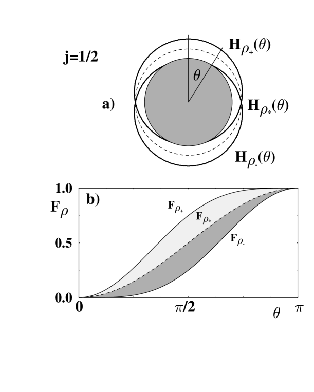
FIG. 4.: a) Cross-section of the Husimi distribution $H_{\rho}(\vartheta)$ for $\rho_{+}$ (peaked at the top), for $\rho_{*}$ (uniform), and for $\rho_{-}$ (peaked at the bottom) plotted for $j=1/2$. b) Monge distance between these states may be represented as the area between graphs of the corresponding distribution functions $F_{\rho_{+}}(\vartheta)$, $F_{\rho_{*}}(\vartheta)$, and $F_{\rho_{-}}(\vartheta)$.

In the case $j=1/2$ all pure states are coherent, so the Monge distance from $\rho_{*}$ is the same for every pure state (as illustrated in Fig. 3). Thus, the manifold of pure states (the Bloch sphere) forms, in the sense of the Monge metric, the sphere $S^{2}$ of radius $R_{1}=\pi/8$ centred at $\rho_{*}$. All mixed states are less localised than coherent and their distance to $\rho_{*}$ is smaller than $R_{1}$. To see this note that every mixed state can be represented as a vector $\bf v$ in the unit ball. Using Proposition 6 and some geometrical considerations one can find the Monge distance between any two mixed states $\rho_{1}$ and $\rho_{2}$. Representing them by Pauli matrices $\vec{\sigma}$ and vectors $\vec{v}_{i}$ in the Bloch ball of radius $1/2$, namely, $\rho_{i}=\rho_{*}+{\vec{\sigma}}\cdot{\vec{v}_{i}}$, we obtain[57]

$$D_{M}(\rho_{1},\rho_{2})=\frac{\pi}{4}\,d({\vec{v}_{1}},{\vec{v}_{2}})=\frac{\pi}{4}|{\vec{v}_{1}}-{\vec{v}_{2}}|\,\text{,}$$ (51)

where $d$ denotes the Euclidean metric in ${\mathbb{R}}^{3}$. Consequently, for $j=1/2$ the Monge distance induces the same geometry as that of the Bloch ball, as illustrated in Fig. 3.

D Monge distances for $j=1$

In an analogous way we treat the case $N=3$. Obtained data

$$R_{1}:=D_{M}(\rho_{+},\rho_{*})=D_{M}(\rho_{-},\rho_{*})=3\pi/16;\quad D_{M}(\rho_{+},\rho_{-})=3\pi/8;$$ (52)

$$R_{2}:=D_{M}(\rho_{*},\rho_{|0\rangle})=1/6;\quad D_{M}(\rho_{+},\rho_{|0\rangle})=D_{M}(\rho_{-},\rho_{|0\rangle})=3\pi/16.$$ (53)

are based on the results derived in Appendix E (see also the next subsection) and visualised in Fig. 5b. Note that both triples $\{\rho_{+},\rho_{*},\rho_{-}\}$ and $\{\rho_{+},\rho_{|0\rangle},\rho_{-}\}$ lay on two different metric lines. Thus, in contrast to the case $j=1/2$, the two states $\rho_{+}$ and $\rho_{-}$ are connected by several different metric lines.

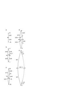
FIG. 5.: Schematic map showing the eigenstates $|j,m\rangle$ and the mixed state $\rho_{*}$ for a) $j=1/2$, b) $j=1$, c) $j=3/2$, d) $j=2$, and e) $j\to\infty$. The symbol $*$ labelling dots represents the maximally mixed state $\rho_{*}$, while numbers $m$ denote pure states $|j,m\rangle$. Solid lines denote the metric lines, and the accompanying numbers represent the approximate Monge distance between the states.

Now, consider a mixed state $\rho_{m}$ represented in the canonical basis by a diagonal density matrix $\rho_{m}=\operatorname*{diag}(a,b,c)$, where $a+b+c=1$. Since $\{\rho_{+},\rho_{|0\rangle},\rho_{-}\}$  lay on a metric line and their distributions are invariant with respect to the horizontal rotation, it is not difficult to calculate the Monge distance $D_{M}(\rho_{+},\rho_{m})$ using Proposition 5. The corresponding distribution functions do not cross, and so $D_{M}(\rho_{+},\rho_{m})=bD_{M}(\rho_{+},\rho_{|0\rangle})+cD_{M}(\rho_{+},\rho_{-})=\linebreak\frac{3\pi}{16}(2-b-2a)$. For comparison $D_{HS}(\rho_{+},\rho_{m})=\sqrt{(1-a)^{2}+b^{2}+(1-a-b)^{2}}$, $D_{tr}(\rho_{+},\rho_{m})=\sqrt{2(1-a)}$, and $D_{Bures}=\sqrt{2(1-\sqrt{a})}$. This simple example shows that for $j=1$ the Monge metrics induces a non-trivial geometry, considerably different from geometries generated by any standard metric.

The Monge distance $R_{\psi}$ between any pure state $|\psi\rangle$ and the mixed state $\rho_{*}$ depends only on the angle $\chi$ between two zeros of the Husimi function located on the sphere. If the zeros are degenerated, $\chi=0$, the state is coherent and $R_{\psi}=R_{1}$. The coherent states are as much localised in the phase space, as allowed by the Heisenberg uncertainty relation. It is therefore intuitive to expect, that out of all pure states the coherent states are the most distant from $\rho_{*}$. In the other extreme case, both zeros lay at the antipodal points, $\chi=\pi$, which corresponds to $\rho_{|0\rangle}$, and $R_{\psi}=R_{2}$. In this symmetrical case, the Husimi distribution is as delocalized as possible, and we conjecture that for every pure state its distance to $\rho_{*}$ is larger than or equal to $R_{2}$.

Thus, considering the Monge distance from $\rho_{*}$, one gets a foliation of the space of pure states ${\cal P}={\mathbb{C}}P^{2}$, as shown in Fig. 6b. As a running parameter we may take the angle $\chi$, which describes a pure state in the stellar representation. This foliation is singular, since the topology of the leaves depends to the angle. The angle $\chi=0$ represents the sphere $S^{2}$ of coherent states ($\sim SO(3)/SO(2)$), intermediate angle represents a generic 3D manifold ${\mathbb{R}}P^{3}/{\mathbb{Z}}_{2}$ (a desymmetrized Stiefel manifold $\sim SO(3)/{\mathbb{Z}}_{2}$) of pure states of the same $\chi$, while the limiting value $\chi=\pi$ denotes the ${\mathbb{R}}P^{2}$ ($\sim SO(3)/O(3)$) manifold of states rotationally equivalent to $\rho_{|0\rangle}$. Similar foliations of ${\cal P}$ discussed in other context may be found in Bacry [54] and in a recent paper by Barros e Sá [58]. For comparison in Fig. 6a we present the foliation of ${\mathbb{C}}P^{1}$ as regards the Monge distance from $\rho_{+}$.

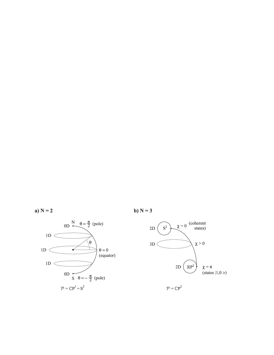
FIG. 6.: Foliation of the sphere along the Greenwich meridian (a), foliation of the four-dimensional space of the $N=3$ pure states along the angle $\chi$ between both zeros of the corresponding Husimi distribution. The poles correspond to the distinguished $2D$ submanifolds of ${\mathbb{C}}P^{2}$: the manifold of coherent states and the manifold of states equivalent to $|1,0\rangle$.

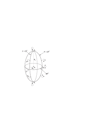
FIG. 7.: Sketch of the structure of the space of the mixed states ${\cal M}$ for $j=1$ induced by the Monge metrics. Manifold of the coherent states ${\cal C}=S^{2}$ is represented by a circle of radius $R_{1}=3\pi/16\sim 0.589$ centred at $\rho_{*}$. Pure states isomorphic to $\rho_{|0\rangle}$ are situated $R_{2}=1/6\sim 0.166$ from $\rho_{*}$. Dots at smaller circles represent the positions of zeros $z_{1}$ and $z_{2}$, which determine each pure state in the stellar representation.

Since it is hardly possible to provide a plot of ${\cal M}$ revealing all details of this non-trivial, $8$-dimensional space of mixed states, we can not expect too much from Fig. 7, which should be treated with a pinch of salt. As it was discussed in Sect. II, from the point of view of the standard metrics, the four-dimensional manifold of the pure states ${\cal P}$ is contained in the sphere $S^{7}$ centered at $\rho_{*}$. For the Monge metric one has $R_{1}>R_{2}$, so we suggest to illustrate ${\cal M}$ as an $8$-dimensional full ‘hyper-ellipsoid’. Pure states $\rho_{+}$ and $\rho_{-}$ occupy its poles along the longest axis. The dashed vertical ellipse represents the space of all coherent states ${\cal C}$, which forms the sphere $S^{2}$ of radius $R_{1}$. Solid horizontal ellipse represents these pure states, which are closest to $\rho_{*}$. This subspace may be obtained from $|0\rangle\langle 0|$ by a three-dimensional rotation of coordinates; topologically it is a real projective space ${\mathbb{R}}P^{2}$. Although both ellipses do cross in the picture, both manifolds do not have any common points, what is easily possible in the four-dimensional space ${\cal P}$. To simplify the identification of single pure states we added in the picture small circles with two dark dots, which indicate their stellar representations. In general, the states represented by points inside the hyper-ellipsoid are mixed. However, since $\cal M$ is only a part of the hyper- ellipsoid, not all points inside this figure do represent existing mixed states.

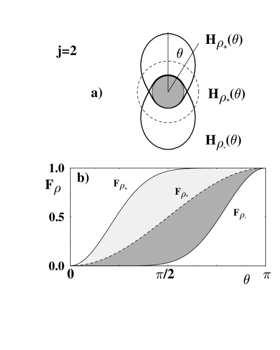
FIG. 8.: As in Fig. 4 for $j=2$.

E The cases: j=3/2 and j=2

For $j=3/2$ ($N=4$) the results read in a simplified notation $D^{(N=4)}_{3/2,1/2}=D^{(N=4)}_{-1/2,-3/2}=5\pi/32$, $D^{(N=4)}_{1/2,-1/2}=9\pi/64$, $D^{(N=4)}_{3/2,*}=D^{(N=4)}_{-3/2,*}=29\pi/128$, and $D^{(N=4)}_{1/2,*}=D^{(N=4)}_{-1/2,*}\simeq 0.2737$. For $j=2$ ($N=5$) one obtains $D^{(N=5)}_{2,1}=D^{(N=5)}_{-1,-2}=35\pi/256$, $D^{(N=5)}_{1,0}=D^{(N=5)}_{0,-1}=15\pi/128$, $D^{(N=5)}_{2,*}=D^{(N=5)}_{-2,*}=65\pi/256$, $D^{(N=5)}_{1,*}=D^{(N=5)}_{-1,*}\simeq 0.3909$, and $D^{(N=5)}_{0,*}=29/120.$ Fig. 5c,d presents a schematic map of these states. Although the results are analytical, we give their numerical approximations, which give some flavour of the geometric structure induced by the Monge metric.

F Monge distances for an arbitrary $j$

1 Eigenstates of ${\bf J_{z}}$

Using the formula for distribution functions $F(\vartheta)$ one may express the distances between neighbouring eigenstates of $J_{z}$ for an arbitrary $j$ by the following formula

$$D_{M}(|j,m\rangle,|j,m-1\rangle)=\pi{2\left(N-n\right)\choose{N-n}}{2n\choose n}2^{-2N}$$ (54)

for $m=-j+1,\dots,j$, where $N=2j+1$ and $n=j+m=1,\dots,N-1$ (for the proof see Appendix E1). This leads to the following asymptotic formula

$$D_{M}(|j,m\rangle,|j,m-1\rangle)\sim\frac{1}{\sqrt{n(N-n)}}$$ (55)

valid for large $j$, where $n$ is defined above. It is easy to show that that for each $j$ all the eigenstates of $J_{z}$ are located on one metric line. Hence we get

$$D_{M}(\rho_{+},\rho_{-})=D_{M}(|j,j\rangle,|j,-j\rangle)=\sum_{m\thinspace=\thinspace-j+1}^{j}D_{M}(|j,m\rangle,|j,m-1\rangle)=\pi\left[1-{\ {{2N\choose N}}}2^{1-2N}\right]\,\text{.}$$ (56)

2 Distance from $\rho_{*}$

According to Property B the distance of each coherent state from $\rho_{*}$ is the same and equal to $R_{1}=D_{M}(\rho_{+},\rho_{*})$. This quantity may be found explicitly for an arbitrary $N=2j+1$:

$$D_{M}(\rho_{+},\rho_{*})=\frac{1}{2}D_{M}(\rho_{+},\rho_{-})=\frac{\pi}{2}\left[1-{\ {{2N\choose N}}}2^{1-2N}\right]\,\text{,}$$ (57)

which is asymptotically (for large $N$) equal to $\pi/2-\sqrt{\pi/N}$. Such a quantity is shown in Fig. 8 (for $j=2$) as the area between two corresponding distribution functions. Observe that in comparison with Fig. 4 the coherent states are more localised, and the area between steeper distribution functions is larger. In the classical limit $N\to\infty$ we arrive at $D_{M}(\rho_{+},\rho_{*})\to\pi/2$ and $D_{M}(\rho_{+},\rho_{-})\to\pi$. The latter result has a simple interpretation: in this limit the coherent states become infinitely sharp and the Monge plan consists in the rotation of the sphere by the angle $\pi$. The three points $\rho_{+}$, $\rho_{*}$, and $\rho_{-}$ form another metric line, which for $N>2$ is different from the metric line generated by the eigenstates of $J_{Z}$. Thus, for $N>2$, the metric induced by the Monge distance is not ‘flat’. Moreover, for $j\in\mathbb{N}$ we have

$$D_{M}(|0\rangle\langle 0|,\rho_{*})=\sum_{k=1}^{j}\allowbreak\frac{1}{2k+1}\frac{\left(2k-1\right)!!}{\left(2k\right)!!}\,\text{,}$$ (58)

which tends to $\pi/2-1$ in the semiclassical limit $j\to\infty$ (for the proof see Appendix E2). It is well known that this convergence is very slow.

3 Coherent states

Now, let us consider two coherent states $|\vartheta,\varphi\rangle$ and $|\vartheta^{\prime},\varphi^{\prime}\rangle$. It follows from the rotational invariance of the Monge metric (Property B) that their distance depends only on $\Xi$ – the angle between two vectors on $S^{2}$ representing these coherent states, and is equal to the Monge distance between two coherent states lying on the Greenwich meridian $\rho_{+}=|0,0\rangle\langle 0,0|$ and $\rho_{\Xi}:=|\Xi,0\rangle\langle\Xi,0|$ (for $N=2$ the latter corresponds to the state labelled in Fig. 3 by $\rho_{\theta}$). We denote this distance by $C(\Xi,j):=D_{M}(\rho_{+},\rho_{\Xi})$. Using Propositions 6 we obtain the following formula for this quantity (for the proof see Appendix E3):

$$C\left(\Xi,j\right)=\pi\,{\sin}\left(\Xi/2\right)W_{j}\left(\sin^{2}\left(\Xi/2\right)\right)\,\text{,}$$ (59)

where $W_{j}$ is a polynomial of the form

$$W_{j}\left(x\right):={{\frac{2j+1}{4^{j+1}}}}\sum\limits_{{}_{\begin{subarray}{c}0\leq u,v\\ u+v<j\end{subarray}}}S_{j,u,v}\,A_{u,v}\,x^{u}\left(1-x\right)^{v}\,\text{.}$$ (60)

The symmetric coefficients $S_{j,u,v}$ are given by

$$S_{j,u,v}:=\frac{\left(2j\right)!}{\left(2j-2\left(u+v\right)-1\right)!u!v!\left(u+v+1\right)!4^{u+v}}\,\text{,}$$ (61)

and the asymmetric coefficients $A_{u,v}$ by

$$A_{u,v}:=\sum_{s=v+1}^{\infty}\frac{\binom{2s}{s}}{\left(u+1+s\right)4^{s}}\,\text{.}$$ (62)

Note that $A_{u,v}$ can be also written as a finite sum

$$A_{u,v}=\frac{2^{2u+1}}{\binom{2u}{u}\left(2u+1\right)}-\sum_{s=0}^{v}\frac{\binom{2s}{s}}{\left(u+1+s\right)4^{s}}\,.$$ (63)

The rank of $W_{j}$ is $\left\lfloor j-1/2\right\rfloor$, i.e., the largest integer less than or equal to $j-1/2$. We have $W_{1/2}\left(x\right)=\allowbreak\frac{1}{4}$ (and so $C(\Xi,1/2)=(\pi/4)\sin(\Xi/2)\sim D_{HS}(\rho_{+},\rho_{\Xi})$), $W_{1}\left(x\right)=\allowbreak\frac{3}{8}$, $W_{3/2}\left(x\right)=\frac{1}{128}\left(57+x\right)$, $W_{2}\left(x\right)=\frac{5}{256}\left(25+x\right)$, etc.

One can show that all the coefficients of the polynomial $W_{j}$ are positive. This leads to the following simple lower and upper bounds

$$\pi\,C_{j}\,\sin\left(\Xi/2\right)\leq C\left(\Xi,j\right)\leq\pi\,D_{j}\,\sin\left(\Xi/2\right)\,\text{,}$$ (64)

where

$$C_{j}:=W_{j}(0)=\frac{j\left(2j+1\right)}{2^{2j+1}}\,_{3}{\mathcal{F}}_{2}\left(\left[3/2,1/2-j,1-j\right],\left[2,2\right],1\right)\,\text{,}$$ (65)

and

$$D_{j}:=W_{j}(1)=\frac{j\left(2j+1\right)}{2^{2j+1}}\,\left(2\cdot\;_{3}{\mathcal{F}}_{2}\left(\left[1,1/2-j,1-j\right],\left[2,3/2\right],1\right)-\;_{3}{\mathcal{F}}_{2}\left(\left[1,1/2-j,1-j\right],\left[2,2\right],1\right)\right)\,\text{.}$$ (66)

(here ${}_{3}{\mathcal{F}}_{2}$ stands for the generalised hypergeometric function). Note that $C_{j}\to 2/\pi$ and $D_{j}\to 1$ in the semiclassical limit $j\to\infty$. For two infinitesimally close coherent states the angle $\Xi\sim 0$ and we get

$$C\left(\Xi,j\right)\sim\frac{\pi}{2}\,C_{j}\,\Xi\,\text{,}$$ (67)

with

$$C\left(\Xi,j\right)\to\Xi\ (j\to\infty)\,\text{,}$$ (68)

which agrees with Property A.

4 Chaotic states

In the stellar representation the coherent states are represented by $N-1$ zeros merging together at the antipodal point on the sphere. These quantum states are rather exceptional; a typical state has all zeros distributed all over the sphere. It is known [59] that for the so-called chaotic states (eigenstates of Floquet operator corresponding to classically chaotic systems) the distribution of zeros is almost uniform in the phase space. Such states are entirely delocalized and their Husimi distribution is close, in a sense of the $L_{1}$ metric, to the uniform Husimi distribution $H_{\rho_{*}}$ corresponding to the maximally mixed state $\rho_{*}$. One can therefore expect (applying Proposition 2) that the Monge distance between these chaotic pure states $\rho_{c}$ and $\rho_{*}$ is small. We conjecture that the mean value of the Monge distance $D_{M}(\rho_{c},\rho_{*})$ of randomly picked chaotic state $\rho_{c}$ from $\rho_{*}$ tends to $0$ in the semiclassical limit $j\to\infty$.

G Correspondence to the Wehrl entropy and the Lieb conjecture

In order to describe the phase space structure of any quantum state $\rho$ it is useful [60] to define the Wehrl entropy $S_{\rho}$ as the Boltzmann–Gibbs entropy of the Husimi distribution (46)

$$S_{\rho}=-\int_{S^{2}}H_{\rho}(\theta,\varphi)\ln[H_{\rho}(\theta,\varphi)]d\mu(\vartheta,\varphi).$$ (69)

It was conjectured by Lieb [61] that this quantity is minimal for coherent states, which are as localised on the sphere as it is allowed by the Heisenberg uncertainty relation. For partial results in the direction to prove this conjecture see [62, 63, 64, 65]. The minimum of entropy reads $S_{\rm min}=(N-1)/N-\ln N$, where the logarithmic term is due to the normalisation of the Husimi distribution. It was also conjectured [63] that the states with possibly regular distribution of zeros on the sphere, which is easy to specify for Pythagorean numbers $N=2,4,6,8,12,20$, are characterised by the largest possible Wehrl entropy among all pure states.

Let us emphasise that for $N>>1$ the states exhibiting small Wehrl entropy comparable to $S_{\rm min}$ are not typical. In the stellar representation coherent states correspond to the coalescence of all $N-1$ zeros of Husimi distribution in one point. In a typical situation all zeros are distributed uniformly on the sphere, and the Wehrl entropy of such delocalized pure states is large. Averaging over the natural Haar measure on the space of pure states $\cal P$ one may compute the mean Wehrl entropy $\langle S\rangle$ for the $N-$dimensional states. In slightly different context such integration was performed in [66, 67, 68] leading to

$$\left\langle S\right\rangle_{U(N)}=-\ln N+\Psi\left(N+1\right)-\Psi\left(2\right)\,\text{,}$$ (70)

where $\Psi$ denotes the digamma function, which for natural arguments $k<n$ satisfies $\Psi(n)-\Psi(k)=\sum_{m=k}^{n-1}1/m$. In the classical limit $N\to\infty$ the mean entropy tends to $\gamma-1\sim-0.42278$ ($\gamma$ is the Euler constant), which is close to the maximal possible Wehrl entropy $S_{\rho_{*}}=0$.

The Wehrl entropy does not induce a metric in the space of quantum states. However, it describes the localisation of a quantum state in the classical phase space and has some properties similar to the Monge distance of a given state $\rho$ to the maximally mixed state $\rho_{*}$ [69]. In view of our results on the Monge distance, we advance analogous conjectures, concerning the set of pure states ${\cal P}$ belonging to the $N-$dimensional Hilbert space.

Conjecture 1.  In the sense of Monge metric the coherent states are pure states most distant from $\rho_{*}$. This maximal distance $R_{1}$ is given by (57) and tends to $\pi/2$ for $N\to\infty$.

Conjecture 2.  Pure states which maximise the Wehrl entropy are the most close to $\rho_{*}$ in the sense of Monge metric. This minimal distance $R_{2}$ is equal to $1/6$ for $N=3$ and tends to $0$ for $N\to\infty$.

In the analogy to the properties of the Wehrl entropy and formula (70), one can expect that the mean distance $\langle R\rangle=\langle D_{M}(|\psi\rangle\langle\psi|,\rho_{*})\rangle$ averaged over the natural measure on the manifold of pure states $\cal P$, is close to the minimal distance $R_{2}$ and, for large $N$, is much smaller than the maximal distance $R_{1}$. In other words, the coherent states, distinguished by the fact of being situated in $\cal M$ as far from $\rho_{*}$ as possible, are not generic. This observation is not surprising, since ${\cal C}\sim{\mathbb{C}}P^{1}$ while ${\cal P}\sim{\mathbb{C}}P^{N-1}$, but is not captured using any standard metrics in the space ${\cal M}$ of mixed quantum states.

V Comparison of Monge and standard distances

Results obtained for distances between several pairs of mixed states are summarised in Table 2. Calculation of the trace, Hilbert-Schmidt and Bures distances are performed directly from the definitions provided in the Sect. I.

Note that the geometry of the space $\cal M$ is well understood for $N=2$. In the sense of the trace and the Hilbert-Schmidt metrics the set of all mixed states has then the property of a ball contained inside the Bloch sphere: the states $\rho_{+},\rho_{*}$ and $\rho_{-}$ form a metric line. The same statement is true for the Monge metric (see formula 51). However, for the Bures metric the situation is different. As it was shown by Hübner the set $\cal M$ has in this case the structure of a half of a $3$- sphere [9], so $\rho_{+},\rho_{*}$ and $\rho_{-}$ form an isosceles triangle. However, the state $\rho_{*}$, located at the pole of $S^{3}$, is equally distant (with respect to Bures metric) from all the pure states ${\cal P}$, which occupy the ‘hyper–equator’ $\sim S^{2}$.

A Geometry of quantum states for large $N$

The data collected in Tab. 2 allow us to emphasise important differences between the geometry induced by the standard distances and the Monge distance. From the points of view of all three of the standard metrics, the distance $R$ between $\rho_{*}$ and any pure state is constant. Therefore, in these standard geometries, the coherent states are not distinguished in any sense in $\cal P$.

On the other hand, a ‘semiclassical’ geometry, induced by the Monge metric in the $(N^{2}-1)-$dimensional space $\cal M$, distinguishes the space of coherent states ${\cal C}\sim S^{2}$. Their Monge distance ($R_{1}$) from the centre $\rho_{*}$ is maximal. If we try to visualise the $(2N-2)-$dimensional space of pure states ${\cal P}\sim{\mathbb{C}}P^{N-1}$ as a ‘hyper-ellipsoid’, the coherent states form the ‘largest circle’, represented by the dashed ellipse in Fig. 9. There exists also a multidimensional subspace of $\cal P$, consisting of delocalized pure states $\rho_{c}$, with zeros of the corresponding Husimi function distributed uniformly on the sphere. Such states are situated close to $\rho_{*}$ with respect to the Monge metric. In the classical limit $N\to\infty$, their distance from $\rho_{*}$ ($R_{2}$) is arbitrary small, so the manifold $\cal P$, almost touches the maximally mixed state $\rho_{*}$. In this case, we might think of $\cal M$ as of a full $(N^{2}-1)-$dimensional disk of radius $R_{1}\sim\pi/2$ centred at $\rho_{*}$, with coherent states at its edge and the pure states on its surface. Since it is rather flat, and contains a lot of its ‘mass’ close to its centre, it resembles, in a sense, the Galaxy.

States $D_{tr}$ $D_{HS}$ $D_{Bures}$ $D_{Monge}$ $(\rho_{+},\rho_{-})$ $2$ $\sqrt{2}$ $\sqrt{2}$ $\pi(1-{\ {{2N\choose N}}}2^{1-2N})\sim\pi-2\sqrt{\pi/N}$ $(\rho_{+},\rho_{\ast})=(\rho_{-},\rho_{\ast})$ $2-\frac{2}{N}$ $\sqrt{1-\frac{1}{N}}$ $\sqrt{2-\frac{2}{\sqrt{N}}}$ $\pi(1/2-{\ {{2N\choose N}}}2^{-2N})\sim\pi/2-\sqrt{\pi/N}$  $\rho_{+},\rho_{\ast},\rho_{-}$  $N=2$ $N>2$ $~{}N\rightarrow\infty~{}$ line isosceles $\Delta$ equilateral $\triangle$ line isosceles $\Delta$ isosceles $\Delta$ isosceles $\Delta$ isosceles $\Delta$ equilateral $\triangle$  line  $(|0\rangle,\rho_{\ast})$  ($j\in\mathbb{N}$) $2-\frac{2}{2j+1}$ $\sqrt{1-\frac{1}{2j+1}}$ $\sqrt{2-\frac{2}{\sqrt{2j+1}}}$ $\sum_{k=1}^{j}\allowbreak\frac{1}{2k+1}\frac{\left(2k-1\right)!!}{\left(2k\right)!!}\to\pi/2-1$ $|m\rangle$, $|m-1\rangle$ $2$ $\sqrt{2}$ $\sqrt{2}$ $\pi{{2\left(N-n\right)}\choose{N-n}}{{2n}\choose{n}}2^{-2N}\sim\frac{1}{\sqrt{N-n}\sqrt{n}}$ ($n=j+m$) $|-j\rangle\cdots|m\rangle\cdots|j\rangle$ $N$-dim simplex $N$-dim simplex $N$-dim simplex line $(\rho_{+},\rho_{a})$ $2(1-a)$ $\sqrt{2}(1-a)$ $\sqrt{2(1-\sqrt{a})}$ $2\pi(1-{\ {{2N\choose N}}}2^{1-2N})(1-a)$ $(\rho_{-},\rho_{a})$ $2a$ $\sqrt{2}a$ $\sqrt{2(1-\sqrt{1-a})}$ $2\pi(1-{\ {{2N\choose N}}}2^{1-2N})a$ $\rho_{+},\rho_{a},\rho_{-}$ line line $\triangle$ line $(\rho_{+},\rho_{\Xi})$ $N=2$ $N\geq 2$ $2\sin(\Xi/2)$ $2\sqrt{1-\cos^{4j}(\Xi/2)}$ $\sqrt{2}\sin(\Xi/2)$ $\sqrt{2-2\cos^{4j}(\Xi/2)}$ $\sqrt{2-2\cos(\Xi/2)}$ $\sqrt{2-2\cos^{2j}(\Xi/2)}$ $(\pi/4)\sin(\Xi/2)$ $C(\Xi,j)=\pi\,{\sin}\left(\Xi/2\right)W_{j}\left(\sin^{2}\left(\Xi/2\right)\right)$ $\to\Xi$ $(\rho_{-},\rho_{\Xi})$ $N=2$ $N\geq 2$ $2\cos(\Xi/2)$ $2\sqrt{1-\sin^{4j}(\Xi/2)}$ $\sqrt{2}\cos(\Xi/2)$ $\sqrt{2-2\sin^{4j}(\Xi/2)}$ $\sqrt{2-2\sin(\Xi/2)}$ $\sqrt{2-2\sin^{2j}(\Xi/2)}$ $(\pi/4)\cos(\Xi/2)$ $C(\Xi,j)=\pi\,{\cos}\left(\Xi/2\right)W_{j}\left(\cos^{2}\left(\Xi/2\right)\right)$ $\to\pi-\Xi$

Table 2. Standard distances (trace, Hilbert-Schmidt and Bures) versus the Monge distance for various quantum states in $N=2j+1$ dimensions - pure states: the coherent states $\rho_{\Xi}=|\Xi\rangle\langle\Xi|$, $\rho_{+}$, $\rho_{-}$, and the eigenstates $|m\rangle$ of $J_{z}$, and mixed states: $\rho_{a}$, defined in Sect. IVB, and the maximally mixed state $\rho_{*}$. For the Monge distance we give semiclassical asymptotics ($N\to\infty$). The polynomials $W_{j}(x)$ are given by formula (60).

B Dynamical properties

As mentioned in Sect. II the standard distances are preserved by the unitary dynamics (see formula (20)). Analogous relation is true for the Monge distance only for some special cases, e.g., for simple rotations $U=\exp(iaJ_{z})$ which preserve the coherence. In general, however, the Monge distance is not conserved

$$D_{M}(\rho_{1},\rho_{2})\neq D_{M}(\rho_{1}^{\prime},\rho_{2}^{\prime})\,\text{.}$$ (71)

Vaguely speaking, during the rotation of the ‘hyper-ellipsoid’, depicted in Fig. 9, a kind of contraction occurs, so the Monge distance changes during the unitary time evolution (and hence is not a monotone metric). Since in the classical limit the distance between coherent states tends to the classical distance on the sphere, we suggested [21] to study the time evolution of the Monge distance $D_{M}(t)$ between two neighbouring coherent states. The quantity $\lambda(t)=\lim_{D_{M}(0)\to 0}(\ln[D_{M}(t)/D_{M}(0)])/t$ characterises indeed the stability of the quantum system. To get a closer analogy with the classical Lyapunov exponent one should then perform the limit $t\to\infty$. However, for longer times, both vector coherent states become delocalized (under the assumption of a generic evolution operator $U$), and their distance to $\rho_{*}$ becomes small. Therefore, after some time $t_{r}$, the distance $D_{M}(t)$ starts to decrease, so instead of analysing $\lim_{t\to\infty}\lambda(t)$ (which always tends to zero), one needs to relay on a finite times quantity $\lambda(t_{r})$ [21, 70].

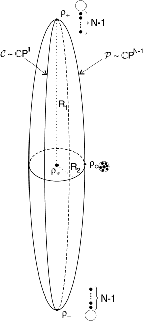
FIG. 9.: Sketch of the space ${\cal M}$ in the semiclassical regime $j>>1$. In the limit $j\to\infty$ the larger radius $R_{1}$ tends to $\pi/2$, while the smaller $R_{2}\to 0$. Dots and small circles show the corresponding pure states in the stellar representation.

C Delocalisation and decoherence

As mentioned above, the localisation of a given pure state $|\phi\rangle$ in the classical phase space is reflected by its large Monge distance from $\rho_{*}$. In an analogous way one may characterise the properties of a given Hamiltonian $H$ or a unitary Floquet operator $F$ by the mean distance of its eigenstates $|v_{i}\rangle,\ i=1,\dots,N$, from the maximally mixed state. Such a quantity, $\gamma:=\sum_{i=1}^{N}D_{M}(|v_{i}\rangle\langle v_{i}|,\rho_{*})]/N$, indicates the average localisation of the eigenstates, relevant to distinguish between integrable and chaotic quantum dynamics [71]. It might be thus interesting to find unitary operators $F_{\min}$ and $F_{\max}$, for which the mean distance $\gamma$ achieves the smallest (the largest) value.

Physical systems coupled to the environment suffer decoherence. The density matrix of a given system tends to be diagonal in the eigenbasis of the Hamiltonian $H_{I}$, which describes the interaction with the environment [72]. In the simplest case, $N=2$, the decoherence may be visualised as an orthogonal projection into an axis determined by $H_{I}$. For example, if $H_{I}$ is proportional to $J_{z}$, it is just the $z$ axis, which joints both poles of the Bloch sphere.

In the general case of arbitrary $N$, there exists an $(N-1)-$dimensional simplex $\cal I$ of density matrices diagonal in the eigenbasis of $H_{I}$. Decoherence consists thus in projecting of the initial state into $\cal I$. In a generic case of a typical interaction the eigenstates of $H_{I}$ are delocalized and their Monge distance from $\rho_{*}$ is small. On the other hand, the typical coherent states are located far away from $\cal I$, in the sense of the Monge metric. One can therefore expect, that the Monge distance of a given quantum state from $\cal I$ contains the information concerning the speed of decoherence. It is known that among all pure states the decoherence of the coherent states is the slowest [73].

Moreover, the speed of decoherence of a Schrödinger cat-like pure state, localised at two different classical points $x$ and $x^{\prime}$, in a generic case depends on their distance in the classical phase space. Consider now a coherent superposition $|\psi\rangle=(|\alpha\rangle+|\beta\rangle)/\sqrt{2}$ of arbitrary two quantum pure states. The Monge distance between them, $D_{M}(|\alpha\rangle,|\beta\rangle)$ might be thus used to characterise the speed of the decoherence of the cat–like state $|\psi\rangle$.

VI Simplified Monge distance between pure states

A Definition

With help of the stellar representation [53, 56, 55] we may link any pure state $|\varphi\rangle$ of the $N$-dimensional Hilbert space to a singular distribution $f_{\varphi}(x)$ containing $(N-1)$ delta peaks placed in the zeros $x_{i}$ of the corresponding Husimi function $H_{|\varphi\rangle\langle\varphi|}(x)$, where $x\in S^{2}$,

$$|\varphi\rangle\to f_{\varphi}(x):={1\over N-1}\sum_{i=1}^{N-1}\delta(x-x_{i}).$$ (72)

The zeros $x_{i}$ may be degenerated. For any coherent state all $(N-1)$ zeros cluster at the antipodal point, so $|\alpha\rangle$ is represented by $f_{\alpha}(x)=\delta(x-{\bar{\alpha}})$.

The simplified Monge distance between any pure states $|\varphi\rangle$ and $|\psi\rangle$ is defined as the Monge distance (23) between the corresponding distributions (72)

$$D_{sM}(|\varphi\rangle,|\psi\rangle):=D_{M}(f_{\varphi},f_{\psi}).$$ (73)

It may be also called discrete Monge distance, since it corresponds to a discrete Monge problem, which may be effectively evaluated numerically by means of the algorithms of linear programming [45]. This contrasts the original definition (31), for which one needs to solve the two dimensional Monge problem for continuous Husimi distributions.

Clearly, in the space of pure quantum states both Monge distances are related. This fact becomes more transparent, if one realises that (73) is equal to the Monge distance between the related distributions ${\bar{f}}_{\varphi}:=[\sum_{i=1}^{N-1}\delta_{{\bar{x}}_{i}}]/(N-1)$ and ${\bar{f}}_{\psi}:=[\sum_{i=1}^{N-1}\delta_{{\bar{y}}_{i}}]/(N-1)$, where $y_{1},\dots,y_{N-1}$ are zeros of the Husimi distribution $H_{|\psi\rangle\langle\psi|}$, and points $x_{i}$ and ${\bar{x}}_{i}$ (resp. $y_{i}$ and ${\bar{y}}_{i}$) are antipodal on the sphere (note that the bar does not denote here the complex conjugation). The distributions ${\bar{f}}_{\varphi}$ and ${\bar{f}}_{\psi}$ may be considered as a discrete, $(N-1)$-points approximation of the continuous Husimi distributions $H_{|\varphi\rangle\langle\varphi|}$ and $H_{|\psi\rangle\langle\psi|}$.

Since any coherent state is represented by a single Dirac delta, ${\bar{f}}_{\alpha}(x)=\delta(x-\alpha)$, the semiclassical condition (8) is exact for any dimension $N$

$$D_{sM}(|\eta_{1}\rangle,|\eta_{2}\ \rangle)=d(\eta_{1},\eta_{2}).$$ (74)

Thus for $N=2$ the discrete Monge distance, $D_{sM}$, is equal to the Fubini-Study distance (7), (in this case, the Riemannian distance $d$ on the sphere), while the continuous Monge metric, $D_{M}$, is proportional to the Hilbert-Schmidt distance (2), (in this case, the Euclidean distance along the cord inside the sphere). At small distances both geometries coincide (the ‘flat earth’ approximation).

B Eigenstates of ${\bf J_{z}}$

In stellar representation the state $|j,m\rangle$ is described by $j+m$ zeros at the south pole and $j-m$ zeros at the north pole. Thus the distribution $f_{j,m}(x)$ consists of two delta peaks, $\pi$ apart, and it is straightforward to obtain the following general result

$$D_{sM}(|j,m\rangle,|j,m^{\prime}\rangle)={\pi\over 2j}|m-m^{\prime}|.$$ (75)

In particular $D_{sM}(|j,j\rangle,|j,-j\rangle)=\pi=d(\alpha,{\bar{\alpha}})$. The zeros of the Husimi function of the eigenstates of the operators $J_{y}$ and $J_{x}$ are located at the equator at the distance $\pi/2$ from both poles. Thus

$$D_{sM}(|j,m\rangle_{z},|j,m^{\prime}\rangle_{y})=D_{sM}(|j,m\rangle_{z},|j,m^{\prime\prime}\rangle_{x})={\pi\over 2}$$ (76)

for any choice of quantum numbers $m,m^{\prime}$ and $m^{\prime\prime}$.

C Random chaotic states

Eigenstates of classically chaotic dynamical systems may be described by random pure states [71]. Expansion coefficients of a chaotic state $|\psi_{c}\rangle$ in an arbitrary basis may be given by a vector of a random unitary matrix, distributed according to the Haar measure on $U(N)$. Zeros of the corresponding Husimi representation are distributed uniformly on the entire sphere [56], (with the correlations between them given by Hannay [74]). This fact allows one to compute the average distance of a random state to any coherent state

$$D_{sM}(|\alpha\rangle,|\psi_{c}\rangle)={1\over 2}\int_{0}^{\pi}\Xi\sin\Xi\ d\Xi={\pi\over 2}.$$ (77)

In a similar way we get the average distance to the eigenstates of $J_{z}$

$$D_{sM}(|j,m\rangle,|\psi_{c}\rangle)=\chi\sin\chi+\cos\chi,\quad{\rm where}\quad\chi={m\pi\over 2j}.$$ (78)

It admits the smallest value equal to unity for $m=\chi=0$, while the largest value is obtained for $m=\pm j$, for which the above formula reduces to (77).

Let us divide the sphere into $N$ cells of diameter proportional to $\sqrt{N}$. Consider two different uncorrelated random states $|\psi_{c}\rangle$ and $|\phi_{c}\rangle$. Uniform distribution of zeros implies that there will be on average one zero in each cell and the distance between the corresponding zeros of both states is of order of $\sqrt{N}$. Thus their simplified Monge distance vanish in the semiclassical limit,

$$D_{sM}(|\psi_{c}\rangle,|\phi_{c}\rangle)\approx{1\over N}{N\over\sqrt{N}}\sim N^{-1/2}\to 0\quad(N\to\infty).$$ (79)

Thus in the space of pure quantum states the simplified, discrete Monge metric $D_{sM}$ displays several features of the original, continuous Monge metric $D_{M}$.

VII Concluding Remarks

In this paper we analysed the properties of the set of all mixed states constructed of the pure states belonging to the $N-$dimensional Hilbert space. The structure of this set is highly non-trivial due to the existence of the density matrices with degenerated spectra. Each spectrum may be represented by a point in the $(N-1)-$dimensional simplex. In a generic case of a nondegenerate spectrum (point located in the interior of the simplex) this set has a structure of $[U(N)/(U(1))^{N}]\times G_{N}$. However, there exist all together $2^{N-1}$ parts of the asymmetric simplex of eigenvalues, all but one corresponding to its boundaries. These boundary points, representing various kinds of the degeneration of the spectrum, lead to a different local structure of the set of mixed states.

Standard metrics in the space of quantum states are not related with the metric structure of the corresponding classical phase space. To establish such a link we used vector coherent states, localised in a given region of the sphere, which plays a role of the classical phase space. Each quantum state may be then uniquely represented by its Husimi distribution, which carries the information concerning its localisation in the classical phase space. We proposed to measure the distance between two arbitrary quantum states by the Monge distance between the corresponding Husimi distributions. Therefore, to compute this distance, one has to solve the Monge problem on the sphere. Thus, unexpectedly, a motivation stemming from quantum mechanics leads us close to the original Monge problem of transporting soil on the Earth surface. Even if the exact solution of the Monge problem is not accessible we can use either lower and upper bounds for the Monge distance (definition (22), Propositions 2 and 4), or numerical algorithms based on the idea of approximation of continuous distributions by discrete ones. These techniques lead to general methods of computing the Monge distance on the sphere (Propositions 5 and 6), as well as to concrete results we obtained in this paper (Sect. IVC,D,E,F and Sect. VA).

The Monge distance induces a non-trivial geometry in the space of mixed quantum states. For $N=2$ it is consistent with the geometry of the Bloch ball induced by the Hilbert-Schmidt or the trace distance. For larger $N$ it distinguishes the coherent states, which are as localised in the phase space, as it is allowed by the Heisenberg uncertainty principle. These states, laying far away from the most mixed state $\rho_{*}$, are not typical. The vast majority of pure quantum states are localised in vicinity of $\rho_{*}$ in the sense of the Monge metric. The Hilbert-Schmidt distance between a given state $\rho$ and $\rho_{*}$ may be used to measure its degree of mixing. On the other hand, the Monge distance $D_{M}(\rho,\rho_{*})$ provides information concerning the localisation of the state $\rho$ in the classical phase space.

A similar geometry in the space of pure quantum states is induced by the simplified Monge metric $d_{sM}$. It is defined by the Monge distance between the $(N-1)$–points discrete approximations to the Husimi representation generated by the stellar representation of pure states. This version of the Monge distance may be easily evaluated numerically by means of the algorithms of linear programming [45]. Therefore it might be used to study the divergence of initially closed pure states subjected to unitary dynamics and to define a quantum analogue of the classical Lyapunov exponent [21, 44]. Moreover, this metric may be useful in an attempt to prove the Lieb conjecture: it suffices to show that for any pure state $|\psi\rangle$ the Wehrl entropy decreases along the line joining $|\psi\rangle$ with the closest coherent state.

In contrast with the standard distances, the both Monge distances are not invariant under an arbitrary unitary transformation. This resembles the classical situation, where two points in the phase space may drift away under the action of a given Hamiltonian system. In a sense, the Monge distance in the space of quantum states enjoys some classical properties. Several classical quantities emerge in the description of quantum systems. We believe, accordingly, that the concept of the Monge distance between quantum states might be useful to elucidate various aspects of the quantum–classical correspondence.

VIII Acknowledgements

K. Ż. would like to thank I. Bengtsson for fruitful discussions and a hospitality in Stockholm. It is a pleasure to thank H. Wiedemann for a collaboration at the early stage of this project and to S. Cynk, P. Garbaczewski, Z. Pogoda, and P. Slater for helpful comments. Travel grant by the European Science Foundation under the programme Quantum Information (K.Ż) and financial support by Polish KBN grant no 2 P03B 07219 are gratefully acknowledged.

A Proof of Proposition 2

Applying Proposition 1 we see that it suffices to prove the inequality

$$\left|\int_{\Omega}f(x)(Q_{1}(x)-Q_{2}(x))dm(x)\thinspace\right|\leq(\Delta/2)D_{L_{1}}(Q_{1},Q_{2})$$ (A1)

for every weak contraction $f:\Omega\to\mathbb{R}$. For such $f$ we see at once that $(\max f-\min f)\leq\Delta$. Let us consider a function $g:\Omega\to\mathbb{R}$ defined by the formula $g(x)=f(x)-\min f-\Delta/2$ for $x\in\Omega$. Clearly $|g|\leq\Delta/2$. Finally, we get

$$\left|\int_{\Omega}f(x)(Q_{1}(x)-Q_{2}(x))dm(x)\thinspace\right|=\left|\int_{\Omega}g(x)(Q_{1}(x)-Q_{2}(x))dm(x)\thinspace\right|\leq(\Delta/2)D_{L_{1}}(Q_{1},Q_{2}),$$ (A2)

which completes the proof.

B Proof of Proposition 4

Let $\rho_{1},\rho_{2}\in\cal{M}$. We denote the set of all contractions ($c-$Lipschitzian functions with $c\leq 1$) $f:\Omega\to\mathbb{R}$ by $Lip_{1}$. We have

$$D_{M}(\rho_{1},\rho_{2})=D_{M}\left({H_{\rho_{1}},H_{\rho_{2}}}\right)=$$ (B1)

$$\max_{f\in Lip_{1}}\left|\int_{\Omega}f(\eta)(H_{\rho_{1}}(\eta)-H_{\rho_{2}}(\eta))dm(\eta)\thinspace\right|=$$ (B2)

$$\max_{f\in Lip_{1}}\left|\int_{\Omega}f(\eta)\langle\eta|(\rho_{1}-\rho_{2})|\eta\rangle dm(\eta)\thinspace\right|=$$ (B3)

$$\max_{f\in Lip_{1}}\left|\operatorname*{tr}\left({\int_{\Omega}f(\eta)|\eta\rangle\langle\eta|dm(\eta)\thinspace(\rho_{1}-\rho_{2})}\right)\right|=$$ (B4)

$$\max\left\{|\operatorname*{tr}A(\rho_{1}-\rho_{2})|:A-\text{Hermitian and}\ A=\int_{\Omega}f(\eta)|\eta\rangle\langle\eta|dm(\eta)\ \text{for some}\ f\in Lip_{1}\right\}=$$ (B5)

$$\max_{L(A)\leq 1}|\operatorname*{tr}A(\rho_{1}-\rho_{2})|\,\text{.}$$ (B6)

C Proof of Proposition 5

We start from two simple lemmas on weak contractions on the sphere. In the sequel, $d$ denotes the Riemannian metric on $S^{2}$.

Lemma 1. Let $f:[0,\pi]\to\mathbb{R}$ be a weak contraction. Define $\widetilde{f}:S^{2}\to\mathbb{R}$ by the formula

$$\widetilde{f}(\vartheta,\varphi)=f(\vartheta)$$ (C1)

for $(\vartheta,\varphi)\in S^{2}$. Then $\widetilde{f}$ is a weak contraction.

Proof of Lemma 1. Let $(\vartheta_{1},\varphi_{1}),(\vartheta_{2},\varphi_{2})\in S^{2}$. Applying spherical triangle inequality we get $|\widetilde{f}(\vartheta_{1},\varphi_{1})-\widetilde{f}(\vartheta_{2},\varphi_{2})|=|f(\vartheta_{1})-f(\vartheta_{2})|\leq|\vartheta_{1}-\vartheta_{2}|\leq d((\vartheta_{1},\varphi_{1}),(\vartheta_{2},\varphi_{2}))$.

Lemma 2. Let $G:S^{2}\to\mathbb{R}$ be a weak contraction. Define $\widetilde{G}:[0,\pi]\to\mathbb{R}$ by the formula

$$\widetilde{G}(\vartheta)=\frac{1}{2\pi}\int_{0}^{2\pi}G(\vartheta,\varphi)d\varphi$$ (C2)

for $\vartheta\in[0,\pi]$. Then $\widetilde{G}$ is a weak contraction.

Proof of Lemma 2. Let $\vartheta_{1},\vartheta_{2}\in[0,\pi]$. We have $d((\vartheta_{1},\varphi),(\vartheta_{2},\varphi))=|\vartheta_{1}-\vartheta_{2}|$. Hence $|\widetilde{G}(\vartheta_{1})-\widetilde{G}(\vartheta_{2})|=(1/2\pi)|\int_{0}^{2\pi}(G(\vartheta_{1},\varphi)-G(\vartheta_{2},\varphi))d\varphi|\leq(1/2\pi)\int_{0}^{2\pi}d((\vartheta_{1},\varphi),(\vartheta_{2},\varphi))d\varphi\leq|\vartheta_{1}-\vartheta_{2}|$.

Proof of formula (47).

It follows from Proposition 1 that

$$D_{M}(\rho_{1},\rho_{2})=D_{M}\left({H_{\rho_{1}},H_{\rho_{2}}}\right)=$$ (C3)

$$\max_{f\in Lip_{1}(S^{2})}\left|\int_{0}^{\pi}\int_{0}^{2\pi}f((\vartheta,\varphi))(H_{\rho_{1}}(\vartheta,\varphi)-H_{\rho_{2}}(\vartheta,\varphi))dm((\vartheta,\varphi))\thinspace\right|=$$ (C4)

$$\max_{f\in Lip_{1}(S^{2})}\left|\int_{0}^{\pi}\left(\int_{0}^{2\pi}f((\vartheta,\varphi))(\tilde{H}_{\rho_{1}}(\vartheta)-\tilde{H}_{\rho_{2}}(\vartheta))\sin{\vartheta}/{4\pi}\thinspace d\vartheta\right)d\varphi\thinspace\right|$$ (C5)

From the Salvemini formula (24), Proposition 1, the above Lemma 1, and formula (C5) we deduce that

$$\int_{0}^{\pi}\left|F_{\rho_{1}}(\vartheta)-F_{\rho_{2}}(\vartheta)\right|d\vartheta=$$ (C6)

$$\max_{f\in Lip_{1}([0,\pi])}\left|\int_{0}^{\pi}f(\vartheta)\left((h_{\rho_{1}}(\vartheta)-h_{\rho_{2}}(\vartheta)\right)d\vartheta\thinspace\right|=$$ (C7)

$$\max_{f\in Lip_{1}([0,\pi])}\left|\int_{0}^{\pi}\left(\frac{1}{4\pi}\int_{0}^{2\pi}\tilde{f}((\vartheta,\varphi))(\tilde{H}_{\rho_{1}}(\vartheta)-\tilde{H}_{\rho_{2}}(\vartheta))\sin{\vartheta}\thinspace d\vartheta\right)d\varphi\thinspace\right|\leq$$ (C8)

$$\max_{f\in Lip_{1}(S^{2})}\left|\int_{0}^{\pi}\left(\frac{1}{4\pi}\int_{0}^{2\pi}f((\vartheta,\varphi))(\tilde{H}_{\rho_{1}}(\vartheta)-\tilde{H}_{\rho_{2}}(\vartheta))\sin{\vartheta}\thinspace d\vartheta\right)d\varphi\thinspace\right|=$$ (C9)

$$D_{M}(\rho_{1},\rho_{2})\,\text{.}$$ (C10)

On the other hand, applying formula (C5), the above Lemma 2, Proposition 1, and the Salvemini formula (24) we get

$$D_{M}(\rho_{1},\rho_{2})=$$ (C11)

$$\max_{G\in Lip_{1}(S^{2})}\left|\int_{0}^{\pi}\left(\int_{0}^{2\pi}G((\vartheta,\varphi))(\tilde{H}_{\rho_{1}}(\vartheta)-\tilde{H}_{\rho_{2}}(\vartheta))\sin{\vartheta}/{4\pi}\thinspace d\vartheta\right)d\varphi\thinspace\right|=$$ (C12)

$$\max_{G\in Lip_{1}(S^{2})}\left|\int_{0}^{\pi}\tilde{G}(\vartheta)\left((H_{1}(\vartheta)-H_{2}(\vartheta)\right)\sin{\vartheta}\thinspace d\vartheta\thinspace\right|\leq$$ (C13)

$$\max_{g\in Lip_{1}([0,\pi])}\left|\int_{0}^{\pi}g(\vartheta)\left(H_{1}(\vartheta)\sin{\vartheta}-H_{2}(\vartheta)\sin{\vartheta}\right)d\vartheta\thinspace\right|=$$ (C14)

$$\int_{0}^{\pi}\left|F_{1}(\vartheta)-F_{2}(\vartheta)\right|d\vartheta\,\text{,}$$ (C15)

which establishes the formula.

D Proof of Proposition 6

Put

$$\widetilde{D}_{M}(\rho_{1},\rho_{2}):=\frac{1}{2\pi}\int_{0}^{2\pi}\int_{0}^{\pi}\left(F_{1}(t,\vartheta)-F_{2}(t,\vartheta)\right)\ dt\ d\vartheta\,.$$ (D1)

Let $\varphi\in\left[0,2\pi\right]$ and $i=1,2$. Integrating by parts we get

$$\int\left(-t\right)\frac{1}{2}H_{\rho_{i}}\left(t,\varphi\right)\sin t\ dt=-tF_{i}\left(t,\varphi\right)+\int F_{i}\left(t,\varphi\right)dt\,\text{.}$$ (D2)

Hence

$$\int\nolimits_{0}^{\pi}\left(F_{1}\left(t,\varphi\right)-F_{2}\left(t,\varphi\right)\right)dt=\int\nolimits_{0}^{\pi}\left(-t\right)\frac{1}{2}\left(H_{\rho_{1}}\left(t,\varphi\right)-H_{\rho_{2}}\left(t,\varphi\right)\right)\sin t\ dt+\left.t\left(F_{1}\left(t,\varphi\right)-F_{2}\left(t,\varphi\right)\right)\right|_{t=0}^{t=\pi}\,\text{.}$$ (D3)

According to assumption (1) the last term is equal to $0$. Thus, applying Proposition 1 to $f:S^{2}\rightarrow\mathbb{R}$ given by $f\left(t,\varphi\right)=-t$, for $t\in\left[0,\pi\right]$, $\varphi\in\left[0,2\pi\right]$, we get

$$\widetilde{D}_{M}\left(\rho_{1},\rho_{2}\right)=\int\nolimits_{0}^{2\pi}\int\nolimits_{0}^{\pi}\left(-t\right)\frac{1}{2}\left(H_{\rho_{1}}\left(t,\varphi\right)-H_{\rho_{2}}\left(t,\varphi\right)\right)\sin t\ dt\ d\varphi\leq D_{M}\left(\rho_{1},\rho_{2}\right)\,\text{.}$$ (D4)

On the other hand consider the following transformation of the density $H_{\rho_{1}}$ into $H_{\rho_{2}}$: we transport the ‘mass’ along each meridian separately (it is feasible due to assumption (1)) and then we join all the transformations together. Applying the Salvemini formula (24) to each meridian ($\varphi\in\left[0,2\pi\right]$), averaging the results over $\left[0,2\pi\right]$, and finally using assumption (2) we get

$$D_{M}\left(\rho_{1},\rho_{2}\right)\leq\frac{1}{2\pi}\int\nolimits_{0}^{2\pi}\int\nolimits_{0}^{\pi}\left|F_{1}\left(t,\varphi\right)-F_{2}\left(t,\varphi\right)\right|\ dt\ d\varphi=\widetilde{D}_{M}\left(\rho_{1},\rho_{2}\right)\,\text{,}$$ (D5)

which completes the proof.

E Derivation of the Monge distances for some interesting cases

1 Derivation of formula (54)

Let $j\in\mathbb{N}$ and $m=-j+1,\dots,j$. We put $N=2j+1$ and $n=j+m$. Applying Proposition 5 and then the substitution $u=\cos^{2}\left(\vartheta/2\right)$ we get

$$D_{M}(|j,m\rangle,|j,m-1\rangle) =\int_{0}^{\pi}\left|\int_{0}^{y}G\left(n,N,\cos^{2}\left(\vartheta/2\right)\right)-G\left(n-1,N,\cos^{2}\left(\vartheta/2\right)\right)\left(\sin\allowbreak\allowbreak\allowbreak\vartheta\right)/2d\vartheta\right|dy$$ (E1)

$$=\int_{0}^{\pi}\left|\int_{\cos^{2}\frac{y}{2}}^{1}G\left(n,N,u\right)-G\left(n-1,N,u\right)du\right|dy\,\text{,}$$ (E2)

where $G\left(n,N,u\right):=N\binom{{N-1}}{n}u^{n}\left(\,1-u\right)^{\left(N-1-n\right)}$ for $u\in\left[0,1\right]$. Using the identity

$$\int\left(G\left(n-1,N,u\right)-G\left(n,N,u\right)\right)du=\binom{{N}}{n}u^{n}\left(\,1-u\right)^{\left(N-n\right)}$$ (E3)

we obtain

$$D_{M}(|j,m\rangle,|j,m-1\rangle) =2\binom{{N}}{n}\int_{0}^{\pi/2}\cos^{2n}v\sin^{2\left(N-n\right)}vdv$$ (E4)

$$=\binom{{N}}{n}\frac{\Gamma\left(n+1/2\right)\Gamma\left(N-n+1/2\right)}{\Gamma\left(N\right)}$$ (E5)

$$=\pi\binom{2\left(N-n\right)}{N-n}\binom{2n}{n}2^{-2N}\sim\frac{1}{\sqrt{N-n}\sqrt{n}}\,\text{,}$$ (E6)

as desired.

2 Derivation of formula (58)

For $j\in\mathbb{N}$ we put $\ D_{j}:=D_{M}(|j,0\rangle,\rho_{\ast})$. From Proposition 5 and formula (47) we deduce that

$$D_{j} =\int_{0}^{\pi}\left|\int_{0}^{\vartheta}h_{|j,0\rangle\left\langle j,0\right|}(\psi)d\psi-\int_{0}^{\vartheta}h_{\rho_{\ast}}(\psi)d\psi\right|d\vartheta$$ (E7)

$$=\int_{0}^{\pi}\left|\int_{0}^{\vartheta}\left(G\left(\cos^{2}\left(\psi/2\right)\right)-1\right)\frac{1}{2}\sin\psi d\psi\right|d\vartheta\,\text{,}$$ (E8)

where $G\left(u\right):=\left(2j+1\right)\binom{{2j}}{j}u^{j}\left(\,1-u\right)^{j}$ for $u\in\left[0,1\right]$. Applying the substitutions $u=\cos^{2}\left(\psi/2\right)$ and $y=\vartheta/2$ and using the symmetry arguments yields

$$\ D_{j} =2\int_{0}^{\pi/2}\left|\int_{\cos^{2}\left(\vartheta/2\right)}^{1}\left(G\left(u\right)-1\right)du\right|d\vartheta$$ (E9)

$$=\text{ }2\int_{0}^{\pi/4}\int_{\sin^{2}y}^{\cos^{2}y}G\left(u\right)\,du\,dy-1$$ (E10)

$$=2\left(2j+1\right)\binom{{2j}}{j}\int_{0}^{\pi/4}\int_{\sin^{2}y}^{\cos^{2}y}u^{j}\left(\,1-u\right)^{j}\,du\,dy-1\,\text{.}$$ (E11)

Set $c_{j}\left(u\right):=2\left(2j+1\right)\binom{{2j}}{j}\int u^{j}\left(\,1-u\right)^{j}du$ for $u\in\left[0,1\right]$, $j\in\mathbb{N}$. Then $D_{j}=\int_{0}^{\pi/4}\left(c_{j}\left(\cos^{2}y\right)-c_{j}\left(\sin^{2}y\right)\right)dy-1$. Integrating by parts we get $c_{j}\left(u\right)=2\binom{{2j}}{j}\left(2u-1\right)u^{j}\left(1-u\right)^{j}+c_{j-1}\left(u\right)$, and so $D_{j}=\binom{{2j}}{j}2^{-2j}\frac{1}{2j+1}+D_{j-1}$. Moreover we can put $D_{0}=0$. Thus $D_{j}=\sum_{k=1}^{j}\allowbreak\frac{1}{2k+1}2^{-2k}\binom{{2k}}{k}=\sum_{k=1}^{j}\allowbreak\frac{1}{2k+1}\frac{\left(2k-1\right)!!}{\left(2k\right)!!}$, as claimed. Applying Taylor’s formula $\arcsin x=\sum_{k=0}^{\infty}\allowbreak\frac{1}{2k+1}\frac{\left(2k-1\right)!!}{\left(2k\right)!!}x^{2k+1}$ we obtain $D_{j}\rightarrow\pi/2-1\,\left(j\rightarrow\infty\right)$.

3 Derivation of formula (59)

Let $C(\Xi,j)=D_{M}(\rho_{+},\rho_{\Xi})$ for $\Xi\in\left[0,\pi\right]$ and $j=1/2,1,...$ . It follows from the rotational invariance of the Monge metric (Property B) that $C(\Xi,j)=D_{M}(\rho_{1},\rho_{2})$, where $\rho_{1}=\rho_{(\pi-\Xi)/2}$ and $\rho_{2}=\rho_{(\pi+\Xi)/2}$. To apply Proposition 6 observe first that according to formula (45) we have

$$H_{\rho_{1}}(\vartheta,\varphi)=\left({2j+1}\right)\left(\frac{{1+\sin\vartheta\cos}\left({\Xi/2}\right){\cos\varphi+\cos\vartheta\sin}\left({\Xi/2}\right)}{2}\right)^{2j}\text{,}$$ (E12)

$$H_{\rho_{2}}(\vartheta,\varphi)=\left({2j+1}\right)\left(\frac{{1+\sin\vartheta\cos\left({\Xi/2}\right)\cos\varphi-\cos\vartheta\sin}\left({\Xi/2}\right)}{2}\right)^{2j}\text{,}$$ (E13)

and so $H_{\rho_{1}}(\vartheta,\varphi)=H_{\rho_{2}}(\pi-\vartheta,\varphi)$ for $(\vartheta,\varphi)\in S^{2}$. Thus, applying the substitution ${\pi-\vartheta\rightarrow\vartheta}$, we get $F_{1}(\pi,\varphi)=\frac{1}{2}\int_{0}^{\pi}H_{\rho_{i}}(\vartheta,\varphi)\sin\vartheta\ d\vartheta=\frac{1}{2}\int_{0}^{\pi}H_{\rho_{2}}(\vartheta,\varphi)\sin\vartheta\ d\vartheta=F_{2}(\pi,\varphi)$, and $F_{1}(t,\varphi)-F_{2}(t,\varphi)=F_{1}(\pi-t,\varphi)-F_{2}(\pi-t,\varphi)$ for $t\in\left[0,\pi\right]$ and $\varphi\in\left[0,2\pi\right]$, which implies the assumption (1). Moreover, $H_{\rho_{1}}(\vartheta,\varphi)-H_{\rho_{2}}(\vartheta,\varphi)\geq 0$ for $\vartheta\in\left[0,\pi/2\right]$ and $\varphi\in\left[0,2\pi\right]$. From this fact and from the symmetry of the functions $F_{1}(\cdot,\varphi)-F_{2}(\cdot,\varphi)$ ($\varphi\in\left[0,2\pi\right]$) we deduce the assumption (2). Hence the assumptions of Proposition 6 are fulfilled and we conclude that

$$C(\Xi,j)={{\frac{{2j+1}}{\pi 4^{j+1}}}}\int_{0}^{2\pi}\int_{0}^{\pi}\left(\int_{0}^{t}\left(\left(w+z\right)^{2j}-\left(w-z\right)^{2j}\right){\sin\vartheta\,d\vartheta}\right)dt\,{d\varphi}\,\text{,}$$ (E14)

where $w:={1+\sin\vartheta\cos\left({\Xi/2}\right)\cos\varphi}$ and $z:={\cos\vartheta\sin\left({\Xi/2}\right)}$. Applying the identity

$$\left(w+z\right)^{2j}-\left(w-z\right)^{2j}=\left\{\begin{tabular}[c]{ll}$2z\sum_{k=0}^{j-1}\binom{2j}{2k+1}w^{2k+1}z^{2j-2k-2}$&\ for $2j$ - even \vskip 6.0pt plus 2.0pt minus 2.0pt\\ $2z\sum_{k=0}^{j-1/2}\binom{2j}{2k}w^{2k}z^{2j-2k-1}$&\ for $2j$ - odd\end{tabular}\right.$$ (E15)

and performing the integration we get after tedious (but elementary) calculation the desired result.

REFERENCES

- [1] Hillery M 1987 Phys. Rev. A 35, 725
- [2] Hillery M 1989 Phys. Rev. A 39, 2994
- [3] Englert B G 1996 Phys. Rev. Lett 77, 2154
- [4] Knöll L and Orłowski A 1995 Phys. Rev. Lett. A 51, 1622
- [5] Wünsche A 1995 Appl. Phys. B 60, S119
- [6] Dodonov V V, Man’ko O V, Man’ko V I and Wünsche A 1999 Physica Scripta 59, 81
- [7] Bures D J C 1969 Trans. Am. Math. Soc. 135, 199
- [8] Uhlmann A 1976 Rep. Math. Phys. 9, 273
- [9] Hübner M 1992 Phys. Lett. A 163, 239
- [10] Uhlmann A 1996 J. Geom. Phys. 18, 76
- [11] Dittmann J 1995 Rep. Math. Phys. 36, 309
- [12] Petz D and Sudár C 1996 J. Math. Phys. 37, 2662
- [13] Uhlmann A 1995 Rep. Math. Phys. 36, 461
- [14] Slater P B 1996 J. Phys. A 29, L271
- [15] Dittmann J 1999 J. Phys. A 32, 2663
- [16] Lesniewski A and Ruskai M B 1999 J. Math. Phys. 40, 5702
- [17] Braunstein S L and Caves C M 1994 Phys. Rev. Lett. 72, 3439
- [18] Wootters W K 1981 Phys. Rev. D 23, 357
- [19] Brody D C and Hughston L P 2001 J. Geom. Phys. 38, 19
- [20] Życzkowski K and Słomczyński W 1998 J. Phys. A 31, 9095
- [21] Życzkowski K, Słomczyński W, and Wiedemann H 1993 Vistas in Astronomy 37, 153
- [22] Husimi K 1940 Proc. Phys. Math. Soc. Jpn. 22, 264
- [23] Dodonov V V, Man’ko O V, Man’ko V I and Wünsche A 2000 J. Mod. Optics 47, 633
- [24] Adelman M, Corbett J V, and Hurst C A 1993 Found. Phys. 23, 211
- [25] Boya L J, Byrd M, Mims M, and Sudarshan E C G 1998 LANL preprint quant-ph/9810084
- [26] Życzkowski K, Horodecki P, Sanpera A, and Lewenstein M 1998 Phys. Rev. A 58, 883
- [27] Slater P 1998 J. Phys. A 32, 5261
- [28] Życzkowski K 1999 Phys. Rev. A 60, 3496
- [29] Poźniak M, Życzkowski K, and Kuś M 1998, J. Phys. A 31, 1059. In this paper a misprint occurred in the algorithm for generating random matrices typical of CUE. The corrected version (indices in the Appendix B changed according to ) can be found in: LANL preprint chao-dyn/9707006
- [30] Hardy G H and Ramanujan S S 1918 Proc. Lond. Math. Soc. 17, 75
- [31] Cassinelli G and Lahti P J 1993 in ’Bridging the Gap: Philosophy, Mathematics, and Physics’ (Springer: Berlin), eds Corsi G et al, pp. 211-224.
- [32] Bush P, Cassinelli G, and Lahti P J 1995 Rev. Math. Phys. 7, 1105
- [33] Bengtsson I 1998 Geometry of quantum mechanics, preprint
- [34] Monge G 1781 Mémoire sur la théorie des déblais et des remblais. Hist. de l’Academie des Sciences de Paris, p. 666
- [35] Rachev S T 1984 Theory Prob. Appl. 29, 647
- [36] Rachev S T 1991 Probability Metrics and the Stability of Stochastic Models (Wiley: New York)
- [37] Sudakov V N 1976 Tr. Mat. Inst. V. A. Steklov, Akad. Nauk SSSR 141 (in Russian)
- [38] Evans L C and Gangbo W 1999 Mem. Amer. Math. Soc. 137
- [39] Kantorovich L V 1942 Dokl. Akad. Nauk SSSR 37, 227
- [40] Kantorovich L V 1948 Uspekhi Mat. Nauk. 3, 225
- [41] Rachev S T and Rüschendorf L 1998 Mass Transportation Problems. Vol. I, Theory (Springer: New York)
- [42] Kantorovich L V 1939 Mathematical Methods in the Organization and Planning of Production. (Leningrad State University: Leningrad); translated in: 1990 Management Science 6, 366
- [43] Salvemini T 1943 Atti della VI Riunione della Soc. Ital. di Statistica, Roma
- [44] Wiedemann H, Życzkowski K, and Słomczyński W 1998 in ’Frontiers in Quantum Physics’, eds Lim S C et al, pp. 240-244, Springer, Berlin.
- [45] Wu N and Coppins R 1981 Linear Programming and Extensions (McGraw-Hill: New York)
- [46] Perelomov A 1986 Generalized Coherent States and Their Applications (Springer: Berlin)
- [47] Thirring W 1980 Lehrbuch der Mathematischen Physik. Band 4: Quantenmechanik grosser Systeme (Springer: Wien)
- [48] Rieffel M A 1999 Doc. Math. 4, 559 (LANL preprint math.OA/9906151 and LANL preprint math.OA/0011063)
- [49] Radcliffe J M 1971 J. Phys. A 4, 313
- [50] Arecchi F T, Courtens E, Gilmore R, and Thomas H 1972 Phys. Rev. A 6, 2211
- [51] Zhang W-M, Feng D H, and Gilmore R 1990 Rev. Mod. Phys. 62, 867
- [52] Vieira V R and Sacramento P D 1995 Ann. Phys. (N.Y.) 242, 188
- [53] Majorana E 1932 Nuovo Cimento 9, 43
- [54] Bacry H 1974 J. Math. Phys. 15, 1686
- [55] Penrose R 1994 Shadows of the Mind (Oxford UP: Oxford)
- [56] Lebœuf P and Voros A 1990 J. Phys. A 23, 1765
- [57] Słomczyński W and Życzkowski K, to be published
- [58] Barros e Sá N 2000 LANL preprint quant-ph/0009022
- [59] Bogomolny E, Bohigas O, and Lebœuf P 1992 Phys. Rev. Lett. 68, 2726
- [60] Wehrl A 1979 Rep. Math. Phys. 16, 353
- [61] Lieb E H 1978 Comm. Math. Phys. 62, 35
- [62] Scutaru H 1979 preprint FT-180/1979 and LANL preprint math-ph/9909024
- [63] Lee C-T 1988 J. Phys. A 21, 3749
- [64] Schupp P 1999 Comm. Math. Phys. 207, 481
- [65] Gnutzmann S and Życzkowski K 2001 LANL preprint quant-ph/0106016
- [66] Kuś M, Mostowski J, and Haake F 1988 J. Phys. A 21, L1073
- [67] Jones K R W 1990 J. Phys. A 23, L1247
- [68] Słomczyński W and Życzkowski K 1998 Phys. Rev. Lett. 80, 1880
- [69] Życzkowski K 2001 Physica E 9, 583
- [70] Haake F, Wiedemann H, and Życzkowski K 1992 Ann. Phys. (Leipzig) 1, 531
- [71] Haake F 2000 Quantum Signatures of Chaos, II ed. (Springer: Berlin)
- [72] Żurek W H 1981 Phys. Rev. D 24, 1516
- [73] Żurek W H 1998 Physica Scripta T 76, 186
- [74] Hannay J H 1996 J. Phys. A 29, L101