On the Problem of Programming Quantum Computers

Abstract

We study effects of the physical realization of quantum computers on their logical operation. Through simulation of physical models of quantum computer hardware, we analyse the difficulties that are encountered in programming physical implementations of quantum computers. We discuss the origin of the instabilities of quantum algorithms and explore physical mechanisms to enlarge the region(s) of stable operation.

I Introduction

The logical operation of a conventional digital computer does not depend on the details of the hardware implementation although the speed of operation and the cost of the machine obviously do. Conventional computers are in one particular state at any time. Furthermore from the point of view of programming the computer, the internal machinery of the basic units comprising the computer is irrelevant. This is very important because it implies that on a conceptual level, algorithms designed to run on a conventional computer will produce answers that do not depend on the hardware that is used.

A quantum computer (QC) is very different in this respect. A QC exploits the fact that a quantum system can be in a superposition of states and that interference of these states allows exponentially many computations to be done in parallel [1, 2, 3, 4, 5]. The presence of this superposition is a manifestation of the internal quantum dynamics of the elementary units (i.e. the qubits). In other words, the quantum dynamics is essential to the operation of a physically realizable QC.

The operation of an ideal QC does not depend on the intrinsic dynamics of the physical qubits: One imagines that the qubits are ideal two-state quantum systems that perform their task instantaneously and perfectly. From a theoretical point of view this situation is very similar to that of computers built from conventional digital circuits. However, in practice there is a fundamental difference. The fact that the logical operation of conventional digital circuits does not depend on their hardware implementation (e.g. semiconductors, relays, vacuum tubes, etc.) is directly related to the presence of dissipative processes that drive the circuits into regions of stable operation. Dissipation suppresses the effects of the internal, non-ideal (chaotic) dynamics of these circuits.

The quantum dynamics of small physical devices is usually very sensitive to small perturbations and this holds for qubits as well. Unfortunately, in contrast to the case of conventional circuits, dissipation usually has a devastating effect on the coherent quantum dynamical motion of the qubits, i.e. on the very essence of QC’s. Therefore the specific physical realization of a QC is intimately related to the stability of its operation.

In this paper we study the relation between the physical realization of QC’s and their logical operation and explore physical mechanisms to enlarge the region(s) of stable operation. We demonstrate that programming a physical implementation of a QC is non-trivial, even if the QC consists of only two or four qubits. In most theoretical work on QC’s and quantum algorithms (QA’s) [5, 6, 7, 8, 9, 10, 11, 12, 13, 14] one considers theoretically ideal (but physically unrealizable) QC’s and therefore this problem of programming QC’s (which we will call the Quantum Programming Problem (QPP)) is not an issue. As far as we know no experimental data has been published that specifically addresses this, for potential applications, very important and intrinsic problem of programming QC’s. The aim of this paper is to investigate various aspects of the QPP by simulating QC hardware.

How does a QPP reveal itself? Consider two logically independent operations ($O_{1}$ and $O_{2}$) of the machine. On a conventional computer or ideal QC, the order in which we execute these two mutually independent instructions does not matter: $O_{1}O_{2}=O_{2}O_{1}$. However, it turns out that on a physically realizable QC sometimes the order does matter, even if there are no dependencies in these two program steps. In some cases $O_{1}O_{2}\not=O_{2}O_{1}$ and the QC may give the wrong answers. The QPP is due to the fact that we are dealing with interacting quantum mechanical objects (as communication between qubits is essential for computation), technical difficulties to manipulate a qubit without disturbing others and the fundamental physical fact that the state of a qubit cannot be frozen during the time that other qubits are being addressed. Also note the qualifier sometimes. There seems to be no general rule to decide beforehand which operation and at what stage of the QA the QPP leads to incorrect results. At present the only way to find out seems to be to actually carry out the calculations and check the results.

It does not require a lot of imagination to see that the QPP implies that it may be very difficult to develop a non-trivial quantum program for a physical QC. Moreover there is no guarantee that a QA that works well on one QC will perform well on other QC’s. Marginal changes in the qubit hardware may affect the interchangeability of logically independent operations. There are several factors that contribute to the QPP:

• Differences between the theoretically perfect and physically realizable one- and two-qubit operations, e.g. the one-qubit operations affecting other qubits and inaccuracies on the time-interval used to perform operations.

• Physical qubits cannot be kept still while others are being addressed.

• The effect of coupling of the qubits to other degrees of freedom (dissipation, decoherence).

In this paper we address these issues through case studies. In Section II we describe the physical model that will be the starting point of our investigations. Our choice of physical models is largely inspired by NMR-QC experiments [15, 16, 17, 18, 19, 20], only because other candidate technologies [21, 22, 23, 24, 25, 26, 27, 28, 29, 30, 31, 32, 33, 34, 35] for building QC’s are not yet developed to the point that they can execute computationally non-trivial QA’s.

As an example of such a QA we will take Grover’s database search algorithm (see Section III) and implement it on various physical models for 2- and 4-qubit QC’s (Sections IV to VI). Our approach for analysing the QPP is to run Grover’s QA by simulating the time-evolution of the physical model representing the QC. Thereby we strictly stick to the rules of quantum mechanics, i.e. we solve the time-dependent Schrödinger equation that describes the evolution of the physical apparatus representing the QC. The main vehicle for performing these simulations is a Quantum Computer Emulator (QCE)[36]. A detailed description of this software tool is given elsewhere [37, 38]. Our work is fundamentally different from those of others who also address questions related to error propagation in QA’s [39, 40, 41, 42] in that we execute QA’s on physical models of QC hardware. The influence of non-resonant effects on the quantum computations using Ising spin quantum computers has been studied by Berman et al. [43]. This work is similar in spirit to the one of the present paper as it explores the consequences of the difference between the ideal and physically realizable QC’s. In this paper we focus on the QPP, not on methods to suppress non-resonant effects. For simplicity most of our calculations (Sections IV and VI) are done for systems at zero temperature, in the absence of interactions with the environment. Simulations of QC’s operating at a non-zero temperature, in contact with a heat bath, are discussed in Section V.

II Physical Model

The simplest qubit is a two-state quantum system, e.g. the spin of electrons or the polarization of photons. The basic operations in a meaningful computation are the manipulation of each qubit (e.g. by applying external fields) and the exchange of information between the qubits. In physical terms, the latter implies that there should be some interaction between the qubits. A non-trivial QC contains at least two qubits. It is known that the most simple spin-1/2 system, i.e. the Ising model, can be used for quantum computing [44, 45, 46]. In the presence of an external magnetic field, the Hamiltonian of the two-spin Ising model reads

$$H=-J_{z}S_{1}^{z}S_{2}^{z}-h_{z}(g_{1}S_{1}^{z}+g_{2}S_{2}^{z}),$$ (1)

where $J_{z}$, $g_{1}$ and $g_{2}$ are material-specific constants, $h_{z}$ represents the applied magnetic field, and $S_{j}^{\alpha}$ denotes the $\alpha$-th component ($\alpha=x,y,z$) of the spin-1/2 operators describing the nuclear spins. In this paper we use units such that $\hbar=1$.

According to the rules of quantum mechanics, the state of the QC at time $t$ is completely described by the wave function $|\Phi(t)\rangle$. Executing a program on a QC is equivalent to solving the time-dependent Schrödinger equation (TDSE)

$$i{\partial\over\partial t}|\Phi(t)\rangle=H(t)|\Phi(t)\rangle.$$ (2)

For the 2-qubit QC the most general linear combination reads

$$|\Phi(t)\rangle=a(\downarrow,\downarrow;t)|\downarrow\downarrow\rangle+a(\uparrow,\downarrow;t)|\uparrow\downarrow\rangle+a(\downarrow,\uparrow;t)|\downarrow\uparrow\rangle+a(\uparrow,\uparrow;t)|\uparrow\uparrow\rangle,$$ (3)

where the $a(b_{1},b_{2};t)$ are complex numbers. The probability that, upon measurement, the QC is in one of the four basis states $|\downarrow\downarrow\rangle,\ldots,|\uparrow\uparrow\rangle$ is given by $|a(\downarrow,\downarrow;t)|^{2},\ldots,|a(\uparrow,\uparrow;t)|^{2}$ respectively.

The final results of a QC calculation can be read off by performing an experiment that measures the expectation value(s) of the spin(s). The value of a qubit is related to the expectation value of the $z$-component of the spin operator:

$$Q_{j}\equiv 1/2-\langle\Phi(t)|S^{z}_{j}|\Phi(t)\rangle\quad;\quad j=1,2,\ldots,N,$$ (4)

where $N$ denotes the total number of qubits of the QC. In this paper we will denote the state of a qubit by

$$|0\rangle\equiv|\uparrow\rangle\quad;\quad|1\rangle\equiv|\downarrow\rangle,$$ (5)

and if necessary we will add a subscript, e.g. $|0\rangle_{1}$, to label the qubit.

The Ising interaction between the spins is sufficient to implement control-NOT (CNOT) gates. Single qubit operations can be performed by applying additional external fields in the $x$ and $y$ direction (see below). It has been shown that any operation involving an arbitrary number of qubits can be written as a sequence of these elementary operations[47], in other words the Ising model is a universal QC.

III Grover’s database search algorithm

Finding the needle in a haystack of $N$ elements requires ${\cal O}(N)$ queries on a conventional computer[48]. Grover has shown that a QC can find the needle using only ${\cal O}(\sqrt{N})$ attempts[9, 10]. Assuming a uniform probability distribution for the needle, for $N=4$ the average number of queries required by a conventional algorithm is 9/4[18, 48]. With Grover’s QA the correct answer can be found in a single query[16, 18]. In general the reduction from ${\cal O}(N)$ to ${\cal O}(\sqrt{N})$ is due to the intrinsic massive parallel operation of the QC.

Experimentally this QA has been implemented on a 2-qubit NMR-QC for the case of a database containing four items[16, 18]. This implementation uses elementary rotations about 90 degrees (clock-wise) around the $x$ and $y$-axis (e.g. ${X_{1}}|00\rangle=(|00\rangle+i|10\rangle)/\sqrt{2}$ etc.) and an interaction-controlled phase shift[16, 18]. It is convenient to express these procedures in matrix notation, for example

$$X_{1}\left(\begin{array}[]{l}|00\rangle\\ |10\rangle\\ |01\rangle\\ |11\rangle\end{array}\right)\equiv{1\over\sqrt{2}}\left(\begin{array}[]{rrrr}1&i&0&0\\ i&1&0&0\\ 0&0&1&i\\ 0&0&i&1\end{array}\right)\left(\begin{array}[]{l}|00\rangle\\ |10\rangle\\ |01\rangle\\ |11\rangle\end{array}\right),$$ (18)

where $|b_{1}b_{2}\rangle\equiv|b_{1}\rangle|b_{2}\rangle$ and $b_{i}=0,1$.

$$Y_{2}\left(\begin{array}[]{l}|00\rangle\\ |10\rangle\\ |01\rangle\\ |11\rangle\end{array}\right)\equiv{1\over\sqrt{2}}\left(\begin{array}[]{rrrr}1&0&1&0\\ 0&1&0&1\\ -1&0&\phantom{-}1&\phantom{-}0\\ 0&-1&0&1\end{array}\right)\left(\begin{array}[]{l}|00\rangle\\ |10\rangle\\ |01\rangle\\ |11\rangle\end{array}\right).$$ (31)

The two qubits “communicate” with each other through the interaction-controlled phase shift

$$I(a)\left(\begin{array}[]{l}|00\rangle\\ |10\rangle\\ |01\rangle\\ |11\rangle\end{array}\right)\equiv{1\over\sqrt{2}}\left(\begin{array}[]{rrrr}e^{-ia/4}&0&0&0\\ 0&e^{+ia/4}&0&0\\ 0&0&e^{+ia/4}&0\\ 0&0&0&e^{-ia/4}\end{array}\right)\left(\begin{array}[]{l}|00\rangle\\ |10\rangle\\ |01\rangle\\ |11\rangle\end{array}\right).$$ (44)

This unitary transformation can be used to implement a CNOT gate. Grover’s algorithm can be expressed entirely by a sequence of the basic operations (18),(31), and (44).

To see how Grover’s QA works it is instructive to consider an example of a database with $N=4$ positions, labeled 0,…,3. Let us assume that the item we are searching for is located at position 2. First we put the QC in its initial state $|00\rangle$. Then we transform this state into the uniform superposition state

$$|u\rangle\equiv{1\over 2}(|00\rangle+|10\rangle+|01\rangle+|11\rangle),$$ (45)

by letting the sequence ${\overline{X}}_{2}{\overline{X}}_{2}{\overline{Y}}_{2}{\overline{X}}_{1}{\overline{X}}_{1}{\overline{Y}}_{1}$ act on $|00\rangle$[18]:

$$|u\rangle={\overline{X}}_{2}{\overline{X}}_{2}{\overline{Y}}_{2}{\overline{X}}_{1}{\overline{X}}_{1}{\overline{Y}}_{1}|00\rangle,$$ (46)

where $\overline{X}_{j}$ ($\overline{Y}_{j}$) denotes the inverse of $X_{j}$ ($Y_{j}$).

Next we apply to $|u\rangle$ the sequence of elementary operations[16, 18, 37, 38]

$$F_{2}\equiv{\overline{Y}}_{1}{X}_{1}{\overline{Y}}_{1}{Y}_{2}{\overline{X}}_{2}{\overline{Y}}_{2}I(\pi),$$ (47)

to encode the content of the database as

$$|\Psi_{2}\rangle={1\over 2}(|00\rangle+|10\rangle-|01\rangle+|11\rangle),$$ (48)

where we adopt the notation in which the basis states are labeled by the binary representation of integers with the order of the bits reversed. In (48) the position of the item in the database (i.e. 2 in this example) is encoded by modifying $|u\rangle$ such that the amplitude of the corresponding basis state changes sign.

The key ingredient of Grover’s algorithm is an operation that determines which of the basis state contributes to (48) with the minus-one amplitude. In matrix notation

$$G={1\over 2}\left(\begin{array}[]{rrrr}-1&1&1&1\\ 1&-1&1&1\\ 1&1&-1&1\\ 1&1&1&-1\end{array}\right),$$ (53)

and in terms of elementary operations

$$G={X}_{1}{X}_{1}{\overline{Y}}_{1}{X}_{2}{X}_{2}{\overline{Y}}_{2}{Y}_{1}{\overline{X}}_{1}{\overline{Y}}_{1}{Y}_{2}{\overline{X}}_{2}{\overline{Y}}_{2}I(\pi){X}_{1}{X}_{1}{\overline{Y}}_{1}{X}_{2}{X}_{2}{\overline{Y}}_{2}.$$ (54)

The sequence (54) is by no means unique: Various alternative expressions can be written down by using the algebraic properties of the $X$’s and $Y$’s. This feature can be exploited to eliminate redundant elementary operations[18]. Starting from the uniform superposition state $|u\rangle$, one choice for the optimized sequences that implement the four different states of the database and Grover’s search algorithm is[16, 18, 37, 38]

$$U_{0} ={X}_{1}{\overline{Y}}_{1}{X}_{2}{\overline{Y}}_{2}I(\pi){X}_{1}{\overline{Y}}_{1}{X}_{2}{\overline{Y}}_{2}I(\pi),$$ (55a)

$$U_{1} ={X}_{1}{\overline{Y}}_{1}{X}_{2}{\overline{Y}}_{2}I(\pi){X}_{1}{\overline{Y}}_{1}{\overline{X}}_{2}{\overline{Y}}_{2}I(\pi),$$ (55b)

$$U_{2} ={X}_{1}{\overline{Y}}_{1}{X}_{2}{\overline{Y}}_{2}I(\pi){\overline{X}}_{1}{\overline{Y}}_{1}{X}_{2}{\overline{Y}}_{2}I(\pi),$$ (55c)

$$U_{3} ={X}_{1}{\overline{Y}}_{1}{X}_{2}{\overline{Y}}_{2}I(\pi){\overline{X}}_{1}{\overline{Y}}_{1}{\overline{X}}_{2}{\overline{Y}}_{2}I(\pi),$$ (55d)

where the $U_{n}$ correspond to the case where the needle is in position $n$.

The sequences of unitary transformations, e.g. $X_{1},Y_{2}$,etc., are easily emulated on an ordinary computer. We use our software package, Quantum Computer Emulator (QCE) [37], to perform these calculations. An example will be shown in Appendix A. On an ideal QC, sequences (55) return the correct answer, i.e. the position of the searched-for item. This is easily verified on the QCE by selecting the elementary operations (called micro instructions on the QCE) that implement an ideal QC.

IV Two-qubit QC’s

The energy-level structure of the nuclear spins of molecules such as deuterated cytosin[15, 16, 49] and carbon-13 labeled chloroform[17, 18] can be described by model (1) and hence they can be used as physical realizations of 2-qubit QC’s.

A Resonant pulses

NMR-QC experiments on carbon-13 labeled chloroform[17] use resonant pulses to manipulate the quantum state of the nuclear spins of the ¹H and ¹³C atoms. In the presence of a static magnetic field along the $+z$ direction this NMR-QC system is described by (1) with $h_{z}g_{1}/2\pi\approx 500\hbox{MHz}$, $h_{z}g_{2}/2\pi\approx 125\hbox{MHz}$, and $J_{z}/2\pi\approx-215\hbox{Hz}$[17]. A detailed account of simulations for this case have been published elsewhere[37, 38]. Simulations for physical model (1) confirm that sequences (55) yield the correct answers for the database search problem[37]. However, we also demonstrated that the outcome of these calculations may be very sensitive to the order in which logically independent operations are carried out[38].. Some of these results are reproduced in Table I (first six rows, for details see [37, 38]).

The results marked with a tilde are obtained by using a logically identical but physically different uniform superposition, i.e.

$$|u^{\prime}\rangle={\overline{X}}_{1}{\overline{X}}_{1}{\overline{Y}}_{1}{\overline{X}}_{2}{\overline{X}}_{2}{\overline{Y}}_{2}|00\rangle.$$ (56)

On an ideal QC, $|u^{\prime}\rangle=|u\rangle$ but on a physical realizable machine this is unlikely to be the case. In an experiment it is simply impossible to freeze spin 2 (1) during the time that resonant pulses are being applied to spin 1 (2). Unless the length of these pulses is chosen judiciously, the wave function will acquire an additional phase. The corresponding unitary transformation does not necessarily commute with the operations that follow, potentially leading to an incorrect final result (as shown in Table I), as we pointed out in a previous paper[38].

For the two-spin system (56) one may optimize the pulse durations such that the effect of these phase errors yields qualitatively correct answers. A basic step is to make the pulse lengths commensurate with all relevant time scales[43, 46]. The main idea of the method suggested in[46] and demonstrated in[43] is to choose the parameters of the electromagnetic pulse such that the non-resonant spin still rotates but returns to its initial position at the end of the pulse [43]. The results of the calculations are shown in Fig. 4 and summarized in Table I (primed symbols)[50]. In the numerical calculations we used $J=-10^{-6}$, $h_{z}g_{1}=1$, $h_{z}g_{2}=0.25$ , ($h_{y}g_{1}=0.025$, $h_{y}g_{2}=0.0625$, $t_{\hbox{pulse}}=4\pi$), for the pulses on the first spin and ($h_{y}g_{1}=0.05$, $h_{y}g_{2}=0.0125$, $t_{\hbox{pulse}}=8\pi$) for the pulses on the second spin, all values in dimensionless units. It is clear that optimization has the desired effect on the sequences that operate on $|u^{\prime}\rangle$ (symbols with a tilde).

In spite of this optimization, Table I shows that there are significant quantitative differences between the theoretically exact results (rows (1,2)) and those obtained by simulating a physical model of a QC (e.g. rows 7 to 10). Even if the pulse length is taken to be commensurate with the relevant time scales of the QC, changing the state of the qubits by way of resonant pulses yields quantum states that are different from those obtained by means of the unitary transformations used in the analysis of the ideal QC. This is because spin 2 also interacts with the field applied to spin 1 and vice versa. With each program step, the non-ideal unitary operation may or may not result in the proliferation of errors. These errors are systematic (there is no “random” error source in our calculations) and directly linked to the structure of the QA. This is a clear case of a QPP, although we managed to let the different QA’s produce the correct answer. Note that the QPP cannot be solved by means of error correction[51]: The operations on the extra qubits required for error correction will suffer from exactly the same QPP.

B Stability of Grover’s quantum algorithm

So far we studied the stability of quantum algorithms by perturbing the input to the database encoding part of the algorithm. In this subsection we will study the QPP of the database query part of Grover’s search algorithm (the operation $G$, see (54)) itself. First we will assume that the input provided to $G$ is exact (i.e. of the form (46) for example) and we will compare the output of logically identical but physically different implementations of $G$. As examples we take the original sequence

$$G={X}_{1}{X}_{1}{\overline{Y}}_{1}{X}_{2}{X}_{2}{\overline{Y}}_{2}{Y}_{1}{\overline{X}}_{1}{\overline{Y}}_{1}{Y}_{2}{\overline{X}}_{2}{\overline{Y}}_{2}I(\pi){X}_{1}{X}_{1}{\overline{Y}}_{1}{X}_{2}{X}_{2}{\overline{Y}}_{2},$$ (57)

and two, logically identical, sequences

$${\hat{G}}={X}_{1}{X}_{1}{\overline{Y}}_{1}{X}_{2}{X}_{2}{\overline{Y}}_{2}{Y}_{1}{\overline{X}}_{1}{Y}_{2}{\overline{X}}_{2}{\overline{Y}}_{1}{\overline{Y}}_{2}I(\pi){X}_{1}{X}_{1}{\overline{Y}}_{1}{X}_{2}{X}_{2}{\overline{Y}}_{2},$$ (58)

$${\tilde{G}}={X}_{1}{X}_{1}{\overline{Y}}_{1}{X}_{2}{X}_{2}{\overline{Y}}_{2}{Y}_{2}{\overline{X}}_{2}{\overline{Y}}_{2}{Y}_{1}{\overline{X}}_{1}{\overline{Y}}_{1}I(\pi){X}_{2}{X}_{2}{\overline{Y}}_{2}{X}_{1}{X}_{1}{\overline{Y}}_{1}.$$ (59)

Note that on purpose we did not “optimize” these sequences by using e.g. ${\overline{X}}_{1}{X}_{1}=1$. On an ideal QC we have[18]

$$G|\Psi_{2}\rangle=G^{3}|\Psi_{2}\rangle={\hat{G}}|\Psi_{2}\rangle={\hat{G}}^{3}|\Psi_{2}\rangle={\tilde{G}}|\Psi_{2}\rangle={\tilde{G}}^{3}|\Psi_{2}\rangle=|01\rangle,$$ (60)

providing another test of the stability of the query operation $G$ on a physical QC. Table II contains the numerical results obtained by running the sequences (57), (58), and (59) on the QCE using the exact state $|\Psi_{2}\rangle$ (see (54)) as input. In the case of the NMR-like QC optimized resonant pulses were used. The ideal QC performs as expected but the physical implementation (symbols with a prime) does not. In fact even one application of ${\tilde{G}}$ apparently returns an answer that is close to being useless ($Q^{\prime}_{1}\approx 0.5$). As the three sequences  (57), (58), and (59) are logically identical this is a clear case of a QPP.

The occurrence of a QPP seems to be a generic feature of QA’s running on QC’s. Therefore it is of interest to try to quantify the QPP. We now describe a simple procedure for this purpose, using $G$ and the case where the item is located in position 0 (the exact input state being $|\Psi_{0}\rangle$) as an example. In general there are two sources of errors in this calculation: The input $|\Psi^{\prime}\rangle$ to $G$ and $G$ itself, the latter depending on the particular hardware implementation of the QC. As before we will use the resonant pulse technique in our numerical experiments.

We write $|\Psi^{\prime}\rangle$ as

$$|\Psi^{\prime}\rangle=\alpha_{0}|\Psi_{0}\rangle+\alpha_{1}|\Psi_{1}\rangle+\alpha_{2}|\Psi_{2}\rangle+\alpha_{3}|\Psi_{3}\rangle,$$ (61)

where the amplitude $\alpha_{0}$ can always be taken real ($-1\leq\alpha_{0}\leq 1$) and is chosen at random. The other three complex coeffients are chosen randomly too, subject to the constraint $|\alpha_{1}|^{2}+|\alpha_{2}|^{2}+|\alpha_{3}|^{2}=1-|\alpha_{0}|^{2}$. The real variable $x\equiv\langle\Psi^{\prime}|\Psi_{0}\rangle=\alpha_{0}$ is a measure for how much the input state deviates from the exact reference input $|\Psi_{0}\rangle$. On an ideal QC, $G|\Psi_{0}\rangle=|00\rangle$. Thus we can use the state $|00\rangle$ as reference to determine how much the output state $|\Theta\rangle\equiv G|\Psi^{\prime}\rangle$ deviates from the exact answer. We quantify this deviation by the variable $y=|\langle 00|G\Psi^{\prime}\rangle|$.

The result of a numerical experiment using 20000 random input states $|\Psi_{0}\rangle$ is shown in Fig. 1. Plots for the three other cases are nearly identical. We classify input-output pairs as “good” or “bad” as follows. First we choose a confidence level $0\leq c\leq 1$ ($c=0.7$ for the data shown in Fig. 1). A particular input-output pair is considered to be good if $x^{2}\geq c$ and $y^{2}\geq c$. In Fig. 1 the good (bad) pairs are shown by black (gray) markers.

At a fairly low confidence level of $c=0.7$, the region of stable operation of the $G$ operation is rather small. This corroborates our earlier finding that successive applications of $G$, e.g. $G^{3}$, rapidly drive the system into a region of instability. In general, quantum systems are very sensitive to noise and become more sensitive as the number of operations on qubits is increased[4]. In the absence of dissipation, it is easy for the system to leave the relatively small manifold of good input states, a characteristic feature of almost chaotic dynamics.

C Hard nonselective pulses

Another physical implementation of a 2-qubit QC employs the nuclear spins of two ¹H spin-1/2 nuclei in a solution of cytosine in D₂O[15, 16, 49]. This system can also be described by Hamiltonian (1). In the NMR experiments hard nonselective pulses are used to address the qubits. In this section we study the stability of QC operation for this physical realization of a QC.

As usual it is expedient to transform to another frame of reference that rotates with a constant frequency. This is accomplished by substituting in the TDSE

$$|\Phi(t)\rangle=e^{ith_{z}(g_{1}+g_{2})(S^{z}_{1}+S^{z}_{2})/2}|\Psi(t)\rangle.$$ (62)

The time evolution of $|\Psi(t)\rangle$ is then governed by the Hamiltonian

$$H=-J_{z}S_{1}^{z}S_{2}^{z}-{\Omega\over 2}S_{1}^{z}+{\Omega\over 2}S_{2}^{z},$$ (63)

where $\Omega=h_{z}(g_{1}-g_{2})$. Guided by experiment[15, 49] in our numerical work we will set $\Omega/2=1$ and $J_{z}/\pi\Omega=-0.01887$ (in dimensionless units).

We now consider the time evolution of the two spins when we apply a static magnetic field $h_{x}$ along the $x$-axis. The Hamiltonian in the laboratory frame is given by

$$H=-J_{z}S_{1}^{z}S_{2}^{z}-h_{z}(g_{1}S_{1}^{z}+g_{2}S_{2}^{z})-h_{x}(g_{1}S_{1}^{x}+g_{2}S_{2}^{x}),$$ (64)

and the corresponding expression in the rotating frame of reference reads

$$H= -J_{z}S_{1}^{z}S_{2}^{z}-{\Omega\over 2}S_{1}^{z}+{\Omega\over 2}S_{2}^{z}$$ (65)

$$-h_{x}(g_{1}S_{1}^{x}+g_{2}S_{2}^{x})\cos\Omega t-h_{x}(g_{1}S_{1}^{y}+g_{2}S_{2}^{y})\sin\Omega t.$$ (66)

If the duration of the pulse is short, i.e. $\Omega t\ll 1$, it is a good approximation to drop the time-dependence in (65) and we obtain

$$\widetilde{H}=-{\Omega\over 2}S_{1}^{z}+{\Omega\over 2}S_{2}^{z}-h_{x}(g_{1}S_{1}^{x}+g_{2}S_{2}^{x}),$$ (67)

where we used the fact that since $|J_{z}|\ll|\Omega/2|$, for short pulses the effect of the spin-spin interaction on the time evolution is small and may be neglected. It is instructive to compute the time evolution of the spins, initially in state $|0\rangle$ ($|0\rangle=|\uparrow\rangle$ by convention), under these circumstances. A straightforward calculation yields

$$Q_{j}=\langle 0|e^{it\widetilde{H}}S_{j}^{z}e^{-it\widetilde{H}}|0\rangle={1\over 2}-{[2h_{x}g_{j}(\Omega/2+\lambda)]^{2}\over[(\Omega/2+\lambda_{j})^{2}+h_{x}^{2}g_{j}^{2}]^{2}}\sin^{2}{\lambda_{j}t\over 2},$$ (68)

where $\lambda_{j}=(\Omega^{2}/4+h_{x}^{2}g_{j}^{2})^{1/2}$. Expression (68) shows that for hard pulses ($|h_{x}g_{j}|\gg\Omega/2$) and $\lambda_{j}t=\pi$, the effect of the pulse is to change qubit $j$ from $|0\rangle$ to approximately $|1\rangle$. Note however that a sequence of such pulses can never turn $|0\rangle$ into $|1\rangle$ exactly and that both spins are affected by the pulse.

In the rotating frame of reference the two spins rotate around the $z$-axis in the opposite sense. This fact can be exploited to perform operations that leave one spin intact while flipping the other spin [49, 52, 53]. For instance, to rotate spin 1 around 90 degrees (clockwise) about the $x$-axis and without changing the state of spin 2, an operation we call $X_{1}$, we can use the sequence of pulses

$${X_{1}^{\phantom{\prime}}}={X_{1,2}^{\prime}}{\overline{Y}_{1,2}^{\phantom{\prime}}}{Z_{1,2}^{\prime}}{Y_{1,2}^{\phantom{\prime}}},$$ (69)

where ${X_{1,2}^{\prime}}$ denotes a 45-degree pulse around the $x$-axis acting simultaneously on both spins (see (67)), ${Y_{1,2}}$ a 90-degree pulse around the $y$-axis, and ${Z_{1,2}^{\prime}}$ represents a pulse during which the spins evolve in time according to (67) and make a rotation of 45 degrees around the $z$-axis, (clockwise in the case of spin 1, anti-clockwise in the case of spin 2). There are many sequences of two-spin pulses that yield $X_{1}$ (or, as a matter of fact, any other rotation). For example the inverse of ${X_{1}^{\phantom{\prime}}}$, ${\overline{X}_{1}^{\phantom{\prime}}}$, can be obtained directly from (69), i.e.

$${\overline{X}_{1}^{\phantom{\prime}}}={\overline{Y}_{1,2}^{\phantom{\prime}}}{\overline{Z}_{1,2}^{\prime}}{Y_{1,2}^{\phantom{\prime}}}{\overline{X}_{1,2}^{\prime}},$$ (70)

or can also be written as

$${\overline{X}_{1}^{\phantom{\prime}}}={\overline{X}_{1,2}^{\prime}}{\overline{Y}_{1,2}^{\phantom{\prime}}}{\overline{Z}_{1,2}^{\prime}}{Y_{1,2}^{\phantom{\prime}}}.$$ (71)

For our numerical calculations we have chosen to work with the sequences

$${X_{1}^{\phantom{\prime}}} ={X_{1,2}^{\prime}}{\overline{Y}_{1,2}^{\phantom{\prime}}}{Z_{1,2}^{\prime}}{Y_{1,2}^{\phantom{\prime}}},$$ (72a)

$${\overline{X}_{1}^{\phantom{\prime}}} ={\overline{X}_{1,2}^{\prime}}{\overline{Y}_{1,2}^{\phantom{\prime}}}{\overline{Z}_{1,2}^{\prime}}{Y_{1,2}^{\phantom{\prime}}},$$ (72b)

$${X_{2}^{\phantom{\prime}}} ={X_{1,2}^{\prime}}{\overline{Y}_{1,2}^{\phantom{\prime}}}{\overline{Z}_{1,2}^{\prime}}{Y_{1,2}^{\phantom{\prime}}},$$ (72c)

$${\overline{X}_{2}^{\phantom{\prime}}} ={\overline{X}_{1,2}^{\prime}}{\overline{Y}_{1,2}^{\phantom{\prime}}}{Z_{1,2}^{\prime}}{Y_{1,2}^{\phantom{\prime}}},$$ (72d)

$${Y_{1}^{\phantom{\prime}}} ={Y_{1,2}^{\prime}}{\overline{X}_{1,2}^{\phantom{\prime}}}{Z_{1,2}^{\prime}}{X_{1,2}^{\phantom{\prime}}},$$ (72e)

$${\overline{Y}_{1}^{\phantom{\prime}}} ={\overline{Y}_{1,2}^{\prime}}{\overline{X}_{1,2}^{\phantom{\prime}}}{\overline{Z}_{1,2}^{\prime}}{X_{1,2}^{\phantom{\prime}}},$$ (72f)

$${Y_{2}^{\phantom{\prime}}} ={Y_{1,2}^{\prime}}{\overline{X}_{1,2}^{\phantom{\prime}}}{\overline{Z}_{1,2}^{\prime}}{X_{1,2}^{\phantom{\prime}}},$$ (72g)

$${\overline{Y}_{2}^{\phantom{\prime}}} ={\overline{Y}_{1,2}^{\prime}}{\overline{X}_{1,2}^{\phantom{\prime}}}{Z_{1,2}^{\prime}}{X_{1,2}^{\phantom{\prime}}},$$ (72h)

to perform the single-qubit operations that are used in the implementation of Grover’s search algorithm. As in the case of resonant pulses the natural time-evolution of the system provides the tool to carry out the conditional phase-shift operation $I(\pi)$.

The numerical values for the qubits 1 and 2 in the final state of the machine, obtained by running the QCE for this particular hardware realization of a QC and QA are are given in Table III.

From a comparison with the data of Table I we conclude that this hardware realization of a 2-qubit QC seems to be much less sensitive to QPP errors. As a matter of fact, in our numerical experiments (data not shown but included in the QCE download) we found none. The main reason for the good performance of this QC can be traced back to the fact that the QC contains two spins with exactly the same precession frequency, precessing in opposite direction. It is clear that it will become rather cumbersome if not impossible to design a $N$-qubit QC (if $N\gg 2$) using this approach: We would have to solve a complicated optimization problem that for each QA we would like to run on the QC.

D Reducing systematic errors

For QC hardware to be of practical use, a basic requirement is that logically identical but physically different implementations of the same QA yield the same answers. The examples discussed above show that optimization of the pulses is essential to achieve this goal. For 2-qubit QC’s, the optimization problem is relatively easy to solve because only two frequencies are involved. Alternatively one may choose to use the same duration for all pulses and optimize the strengths of the pulses. However, in the case of $N\gg 2$ qubits, choosing pulse durations commensurate with $N$ different frequencies will considerably slow down the operation of the whole machine. In addition, the longer the pulses, the more important the effect of imperfections of the pulses becomes. Although there are ingenious techniques to optimize pulses in this respect[52, 54, 55, 56], it may well be that in order to successfully run a QA on $N$-qubit QC hardware one first has to solve a rather complicated optimization problem and then simulate the QC by running the QA on a conventional machine.

V Can dissipation reduce the QPP ?

Elsewhere we reported on the effect of dissipation on the quantum dynamics of nanoscale magnets[57, 58]. In these systems dissipation usually causes decoherence. Decoherence limits the time for performing quantum computations. Above we have demonstrated that programming non-ideal QC’s is difficult due to intrinsic instabilities of the physical device. Therefore we wonder if dissipation can provide the stabilizing processes, perhaps at the cost of reducing the time of coherent quantum operation.

Let us consider the procedure to generate the uniform superposition state from the state with all spins up. Above we made use of sequences such as $XXY$ but it is easy to see that from a programming-point-of-view $Y$ is just as good: In a classical picture both sequences change the direction of a spin from the $z$ to the $x$-axis. Thus, on an ideal QC we may omit $XX$ if we want. However, in an experiment (in which there always is some amount of dissipation), $XX$ can help to stabilize the direction of the spin once it points in the $x$-direction. Although in the pure quantum case $XX$ only causes the spin to precess around the $x$-axis, the damping of this motion by dissipation will let the spin relax to the $x$-direction.

We have studied the effects of dissipation on quantum computations using the master equation[59]

$${\partial\rho(t)\over\partial t}=-i[H,\rho(t)]-\lambda\left([C,R\rho(t)]+[C,R\rho(t)]^{\dagger}\right),$$ (73)

that describes the time-evolution of the reduced (to the subspace of the qubits) density matrix $\rho(t)$. The operator $R$ is defined as

$$\langle k|R|m\rangle=\zeta(E_{k}-E_{m})N_{\beta}(E_{k}-E_{m})\langle k|C|m\rangle,$$ (74)

where $H|k\rangle=E_{k}|k\rangle$, $H$ being the Hamiltonian describing the QC. We take for the spectral density of the bosonic thermal bath $\zeta(E)=I_{0}E^{2}\hbox{sign}(E)$, i.e. an super-Ohmic reservoir, and $N_{\beta}(E)=(e^{\beta E}-1)^{-1}$ denotes the boson occupation number[60]. The operator $C$ specifies the coupling between the spins and the bosons, e.g. $C=\sum_{j}(S_{j}^{x}+S_{j}^{z})/2,$. We set the inverse temperature $\beta=100$[61]. The parameter $\lambda$ controls the flow of heat to and from the QC.

The procedure for simulating a QC in the presence of dissipation is very similar to the one used in the pure quantum case: The only difference is that we solve the master equation (73) instead of TDSE (2). For $\lambda=0$ the two completely different numerical methods used to solve these two equations (see [60] and [37] respectively) yield identical results.

We have studied the effect of dissipation by performing calculations for the same cases as described in Section IV A. Our simple-minded model of dissipation is found to cause only decoherence. We don’t find qualitative differences between the time-evolutions corresponding to the two different initial conditions. The presence of dissipation does not seem to affect the QPP. For $\lambda=10^{-5}$ the value of the qubits in the final states is approximately 1/2, i.e. all useful information is lost (see Fig. 2). Apparently our choice does not lead to a relaxation during the $XX$ pulses. Although the dissipation processes incorporated through the use of master equation (73) lead to the correct thermal equilibrium state, there is no unique prescription to choose the bath Hamiltonian and the coupling between the bath and the spin system, i.e. the form of $C$. We are currently studying more realistic mechanisms for dissipation and will report on the results elsewhere.

VI Four-qubit QC’s

In general practical applications of QC’s will require complicated QA’s. Therefore it is of interest to study how the instabilities due to imperfections in the operations affect the performance in such complicated QA’s. In this section we use a copy (or swap) procedure in a four-qubit QC as one of the simplest examples.

As discussed above, an implementation of Grover’s search algorithm on a QC consist of two separate parts: 1) The preparation of the uniform superposition state $|u\rangle$ and encoding of the database information and 2) the search (query) of the database. The algorithms described above use the same two qubits for these two different tasks. First they are used to store the information contained in the database and second they are used to carry out Grover’s algorithm to query the very same two qubits. Although this is sufficient to demonstrate the realization of 2-qubit QC hardware, from the point of view of computation this demonstration is of little use. Indeed, instead of organizing the computation in two steps (bringing the two qubits into a state that reflects the content of the database and then using the same two qubits to perform the query) we could have written the information from the database directly into the qubits in a form which reveals the position of the item in a trivial manner.

A computationally non-trivial demonstration of a QC running Grover’s database search algorithm requires the database and quantum processor to have their own qubits. This obviously means using at least four qubits, two to hold the database information (in superposition state) and two to process the query. Therefore we will need an operation to copy the state of the database into the quantum processor. A schematic picture of how the calculation is organized is shown in Fig. 3. Let us now study how instabilities in the physical operations affect the outcome of this more complicated computational procedure.

The copy operation transfers the amplitudes of an arbitrary linear combination of spin-up and spin-down of e.g. spin 1 to e.g. spin 2, initially in a state of spin up. More specifically

$$C_{1,2}(a|0\rangle_{1}+b|1\rangle_{1})|0\rangle_{2}=|0\rangle_{1}(a|0\rangle_{2}+b|1\rangle_{2}).$$ (75)

In principle this can be done by a network of CNOT gates[3]. One possible realization of a CNOT gate is the pulse sequence

$$C_{1,2}={Y}_{1}{X}_{1}{Y}_{1}{X}_{1}{\overline{Y}}_{1}{X}_{2}{\overline{Y}}_{2}I(\pi){Y}_{2},$$ (76)

up to irrelevant phase factors, but there are many others. A fundamentally different sequence that performs the same task is

$$C_{1,2}={Y}_{2}{\overline{X}}_{2}{\overline{Y}}_{2}I^{\prime}(\pi),$$ (77)

where

$$I^{\prime}(2a)\left(\begin{array}[]{l}|00\rangle\\ |10\rangle\\ |01\rangle\\ |11\rangle\end{array}\right)\equiv\left(\begin{array}[]{cccc}1&0&0&0\\ 0&\cos a&i\sin a&0\\ 0&i\sin a&\cos a&0\\ 0&0&0&1\end{array}\right)\left(\begin{array}[]{l}|00\rangle\\ |10\rangle\\ |01\rangle\\ |11\rangle\end{array}\right).$$ (90)

A simple calculation shows that the two-qubit operation $I^{\prime}(2a)$ corresponds to the time-evolution of a two-spin XY model:

$$I^{\prime}(2\tau J_{xy})=e^{-i\tau J_{xy}(S_{1}^{x}S_{2}^{x}+S_{1}^{y}S_{2}^{y})}.$$ (91)

The other pulses in sequence (77) serve to remove unwanted phase factors. Note that (75) and (91) destroy the state of the database, a manifestation of the “no-cloning theorem”[62]. As Fig. 3 shows this is not really a problem as the state of the database after the copy operation took place is the same state that was used to initialize the state of the database.

As before our aim is to address the fidelity of the results obtained by running a quantum algorithm on a hardware realization of a QC. Our QCE can simulate various candidate technologies and architectures (ways of interconnecting different units). However, to analyse the QPP it is at present sufficient to consider marginal extensions of two-qubit QC’s. With this in mind we have chosen to “implement” a 4-qubit QC as two identical Ising models

$$H=-J_{z}S_{1}^{z}S_{2}^{z}-h_{z}(g_{1}S_{1}^{z}+g_{2}S_{2}^{z})-J_{z}S_{3}^{z}S_{4}^{z}-h_{z}(g_{1}S_{3}^{z}+g_{2}S_{4}^{z}).$$ (92)

In our numerical work we take for the values of the model parameters those corresponding to the chloroform molecule and we use selective resonant pulses to address the individual spins (see above). Thereby we assume, again for simplicity of analysis, that we can address pairs (1,2) and (3,4) separately (i.e. a pulse tuned to spin 1 does not affect spin 3 etc.). In the case where we use CNOT’s to perform the copy-qubit operation we add to (92) the Ising interactions

$$H_{1,3} =-J_{z}S_{1}^{z}S_{3}^{z},$$ (93a)

$$H_{2,4} =-J_{z}S_{2}^{z}S_{4}^{z},$$ (93b)

or, in the case the XY-model is used to copy the qubits from the database into the query processor, we add to (92)

$$H_{1,3}^{\prime} =-J_{xy}(S_{1}^{x}S_{3}^{x}+S_{1}^{y}S_{3}^{y}),$$ (94a)

$$H_{2,4}^{\prime} =-J_{xy}(S_{2}^{x}S_{4}^{x}+S_{2}^{y}S_{4}^{y}).$$ (94b)

It is obvious that these operations cannot be realized in terms of NMR technology. However this extension from a 2-qubit to a 4-qubit QC is sufficient to study in detail the stability of QA’s.

A Resonant pulses

In our numerical simulations on the QCE we take the same model parameters as those of the chloroform molecule (see above) for both the database and query machine. We use resonant pulses to address the single qubits. Thereby we assume that qubits 1 and 2 can be shielded from qubits 3 and 4 during the application of these pulses.

The results of running Grover’s search algorithm on the QCE are summarized in Table IV. In these calculations we used the pulses optimized in the sense discussed above (i.e. when used to run on a 2-qubit QC they yield the correct answers, independent of the initialization sequence). Nevertheless we observe that the implementation that uses the CNOT gates performs rather poorly, at the border of giving the wrong answers. As in the 2-qubit case, the fact that the duration of the pulses is no longer commensurate with the Larmor periods of the spins is one source of errors. Another mechanism that causes errors to accumulate is discussed below.

B Rotating field

Finally, in an attempt to further reduce the uncertainty on the outcome of the quantum computations, we have repeated the simulations using resonant pulses of rotating fields[63, 64]. More specifically, to apply a pulse to rotate for example spin 1, we add to the Hamiltonian a term of the form

$$H_{1}(t)=h_{1}S_{j}^{y}\sin f_{1}t+h_{1}S_{j}^{x}\cos f_{1}t,$$ (95)

where the frequency $f_{1}$ is tuned to the resonance frequency of spin 1 and the intensity of the pulse $h_{1}$ is determined by the desired angle of rotation. A simple calculation shows that such a pulse transforms the single qubit in exactly the same manner as the corresponding, ideal transformation[63, 64]. It is evident that this kind of optimization should improve the stability of the QA with respect to logically-allowed interchanges of operations. Further improvements can be made by reordering some of the elementary operations (recall that the sequence implementing e.g. a CNOT is not unique). The results of the simulations are presented in Table V. Compared to the results of Table IV there is one major change: The CNOT based implementation performs much better.

In this implementation there are two sources of errors: The effect of the pulses on non-resonant spins and the interaction-controlled phase shift. In the case of the chloroform molecule there is a large difference in time scale (roughly a factor $10^{6}$) between the precession frequencies and the spin-spin interaction. Therefore, during the execution of an interaction-controlled phase shift, the spins make a large number of rotations about the $z$-axis. We have seen that it really matters for the stability of the calculation whether the angles of rotation are a multiple of $2\pi$ or not. However, in view of the difference in time scale, this implies that the duration of an interaction-controlled phase shift must be specified with a sufficiently high accuracy in order to recover the correct final results.

VII Summary

We have studied the difficulties that are encountered in programming quantum computer hardware. Taking Grover’s database quantum search algorithm as an example, we ran various, logically identical versions of the algorithm on different, physically realizable quantum computer hardware. We demonstrated that the choice of the physical processes used for quantum computation has direct consequences in terms of programming the machine.

We have shown that in the absence of dissipation non-ideal, physically realizable quantum computers operate in a regime of extreme sensitivity. This high sensitivity reflects itself in problems of programming quantum computers such that they perform correct calculations. These problems cannot be solved by error correction but may be reduced, and in some cases almost eliminated, at the cost of extensive, machine and program-specific optimization. A possible route to reduce this sensitivity may be to introduce some form of dissipation in a well-controlled manner. Dissipation can extend the region of stable operation of the quantum computer but also limits the time interval for quantum computer operation due to decoherence. We are currently exploring ideas along this line.

A Quantum Computer Emulator (QCE)

In this appendix, we show an example of QCE. In Fig. 4 we show a snapshot of a window of QCE with a set of operations used to produce the results of Table I for the optimized pulses.

The left panel in Fig. 4 lists the fundamental operations, where MI stands for micro instruction. For example MI ‘-X1’ means the operation ${\bar{X}_{1}}$, etc. MI’s are defined by a table with interaction parameters, duration time, etc. This table appears when we double-click an MI. More details can be found in [37]. The set of MI’s for the case of resonant optimized pulses is stored under the name ‘nmr-insta’. A QP represents a subroutine which consist of sequence of MI’s. For example QP ‘f2’ means the sequence of operations $F_{2}$, see Eq. (47). The MI ‘initialize’ simply prepares the state $|00\rangle$, MI ‘inv-means’ performs the inversion about the mean (the essential step in Grover’s algorithm, see Eq. (53)), MI ‘tau’ corresponds to the operation $I(\pi)$ (see Eq. (44)), QP ‘prepare’ denotes the preparation of $|u\rangle$ while QP ‘prapera’ denotes the preparation of $|u^{\prime}\rangle$, etc. The MI’s ‘tau2’, ‘tau_insta’, and ‘w1’ are not used in this example.

The eight small windows show the programs corresponding to $U_{0},\cdots U_{3}$ using $|u\rangle$ (upper level) and those using $|u^{\prime}\rangle$ (lower level), which are named QP ‘g0’ to QP ‘g3prap1̃’. The result of running each program is shown in the grid below the QP. The expectation value of $(1-S_{i}^{\alpha})/2$, $i=1$ or 2, and $\alpha=x,y$ or z, can be read off from a particular cell by moving the mouse over the cell (not shown). In Fig. 4 the approximate value can be determined from the darkness of the cell: Light gray corresponds to zero, dark gray to one. For example, the value of the cell $(z,1)$ in QP ‘g0’ is 0.027 and that of $(z,2)$ is 0.152, as given in Table I ($Q_{1}^{\prime}$ and $Q_{2}^{\prime}$ respectively). For other cases, e.g. the non-optimized pulses, we use another set of MI’s (‘nmr’) with parameters given in [37].

TABLE I.: Final state of the qubits after running the Grover’s database search algorithm on an ideal QC ($Q_{1},Q_{2}$), on a NMR-like QC ($\hat{Q}_{1},\hat{Q}_{2}$), and on the same QC ($\tilde{Q}_{1},\tilde{Q}_{2}$) using a different, but logically identical, initialization sequence ($|\overline{u}\rangle=|u^{\prime}\rangle$ instead of $|\overline{u}\rangle=|u\rangle$). The optimized results, marked with a prime, have been obtained by changing the duration and intensity of the pulses tuned to the resonance frequency of spin 1 by a factor of two and 1/2 respectively.

	$U_{0}|\overline{u}\rangle$	$U_{1}|\overline{u}\rangle$	$U_{2}|\overline{u}\rangle$	$U_{3}|\overline{u}\rangle$
$Q_{1}$	0	1	0	1
$Q_{2}$	0	0	1	1
$\hat{Q}_{1}$	0.028	0.966	0.037	0.995
$\hat{Q}_{2}$	0.163	0.171	0.836	0.830
$\tilde{Q}_{1}$	0.955	0.041	0.971	0.027
$\tilde{Q}_{2}$	0.031	0.026	0.971	0.972
$\hat{Q}_{1}^{\prime}$	0.027	0.972	0.037	0.964
$\hat{Q}_{2}^{\prime}$	0.152	0.180	0.847	0.820
$\tilde{Q}_{1}^{\prime}$	0.030	0.969	0.034	0.965
$\tilde{Q}_{2}^{\prime}$	0.022	0.035	0.977	0.965

TABLE II.: Final state of the qubits after running the query part $G$ of Grover’s database search algorithm on an ideal QC ($Q_{1},Q_{2}$) and on a NMR-like QC ($Q_{1}^{\prime},Q_{2}^{\prime}$). In all cases the input state $|\Psi_{2}\rangle$ corresponds exactly to the case where the item is located in position 2 in the database. The queries ${\hat{G}}$ and ${\tilde{G}}$ are logically identical to $G$. The differences in the outputs of the NMR-like QC are due to the internal quantum dynamics of the physical qubits used.

	$G|\Psi_{2}\rangle$	${\hat{G}}|\Psi_{2}\rangle$	${\tilde{G}}|\Psi_{2}\rangle$	$G^{3}|\Psi_{2}\rangle$	${\hat{G}}^{3}|\Psi_{2}\rangle$	${\tilde{G}}^{3}|\Psi_{2}\rangle$
$Q_{1}$	0	0	0	0	0	0
$Q_{2}$	1	1	1	1	1	1
$Q_{1}^{\prime}$	0.257	0.154	0.487	0.908	0.766	0.578
$Q_{2}^{\prime}$	0.944	0.944	0.988	0.938	0.857	0.995

TABLE III.: Final state of the QC after running the Grover’s database search algorithm on an ideal QC ($Q_{1},Q_{2}$) and an QC ($\hat{Q}_{1},\hat{Q}_{2}$) using hard, non-selective pulses. ($\tilde{Q}_{1},\tilde{Q}_{2}$): QC using hard non-selective pulses, and a different but logically identical initialization sequence ($|\overline{u}\rangle=|u^{\prime}\rangle$ instead of $|\overline{u}\rangle=|u\rangle$).

	$U_{0}|\overline{u}\rangle$	$U_{1}|\overline{u}\rangle$	$U_{2}|\overline{u}\rangle$	$U_{3}|\overline{u}\rangle$
$Q_{1}$	0	1	0	1
$Q_{2}$	0	0	1	1
$\hat{Q}_{1}$	0.000	0.999	0.001	0.999
$\hat{Q}_{2}$	0.000	0.005	0.999	0.996
$\tilde{Q}_{1}$	0.001	0.999	0.002	0.999
$\tilde{Q}_{2}$	0.001	0.002	0.999	0.998

TABLE IV.: Final state of the QC after running the Grover’s database search algorithm on a 4-qubit QC. $Q_{3},Q_{4}$: ideal QC; $\hat{Q}_{3},\hat{Q}_{4}$: NMR-like QC, using an XY-model time-evolution to copy the state of the database to the two-qubit QC that performs the query; $\tilde{Q}_{3},\tilde{Q}_{4}$: NMR-like QC, using a sequence of CNOT to perform the copy operations. The values of the two database qubits are not shown.

	$U_{0}|u\rangle$	$U_{1}|u\rangle$	$U_{2}|u\rangle$	$U_{3}|u\rangle$
$Q_{3}$	0	1	0	1
$Q_{4}$	0	0	1	1
$\hat{Q}_{3}$	0.172	0.809	0.190	0.831
$\hat{Q}_{4}$	0.135	0.187	0.865	0.814
$\tilde{Q}_{3}$	0.412	0.565	0.433	0.591
$\tilde{Q}_{4}$	0.113	0.218	0.888	0.783

TABLE V.: Final state of the QC after running the Grover’s database search algorithm on a 4-qubit QC, using pulses optimized to reduce the effect of imperfections of the operations and phase errors. $Q_{3},Q_{4}$: ideal QC; $\hat{Q}_{3},\hat{Q}_{4}$: NMR-like QC, using an XY-model time-evolution to copy the state of the database to the two-qubit QC that performs the query; $\tilde{Q}_{3},\tilde{Q}_{4}$: NMR-like QC, using a sequence of CNOT to perform the copy operations. The values of the two database qubits are not shown.

	$U_{0}|u\rangle$	$U_{1}|u\rangle$	$U_{2}|u\rangle$	$U_{3}|u\rangle$
$Q_{3}$	0	1	0	1
$Q_{4}$	0	0	1	1
$\hat{Q}_{3}$	0.195	0.806	0.193	0.806
$\hat{Q}_{4}$	0.195	0.194	0.805	0.806
$\tilde{Q}_{3}$	0.265	0.737	0.262	0.737
$\tilde{Q}_{4}$	0.197	0.193	0.804	0.807

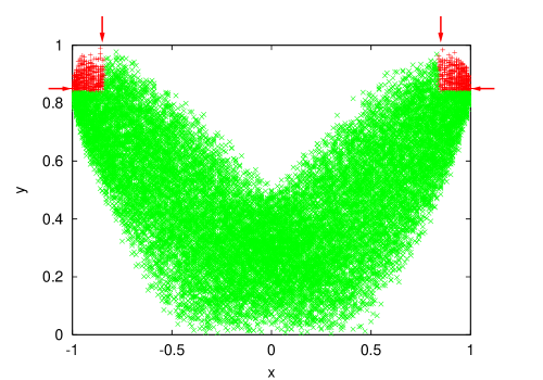
FIG. 1.: Region of stable (black) and unstable (gray) operation of Grover’s search algorithm when executed on a 2-qubit NMR-like QC. The $x$-coordinate ($x=\langle\Psi^{\prime}|\Psi_{0}\rangle$) gives the projection of the random input state $|\Psi^{\prime}\rangle$ on the exact input state $\Psi_{0}$, i.e. for the case where the item is at position 0. The $y$-coordinate ($y=|\langle 00|G\Psi^{\prime}\rangle|$) discriminates between correct and false output. A confidence level of $c=0.7$ on the input-output pair was used to determine if $G$ yields the correct result. The horizontal (vertical) arrows mark the values of $y$ ($x$) at which the input (output) state is equal to its ideal value. Note the absence of points in the regions near $(-1,1)$ and $(1,1)$.

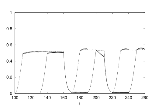
FIG. 2.: Time evolution of the qubits $\tilde{Q}_{1}^{\prime}$ (solid line) and $\tilde{Q}_{2}^{\prime}$ (dashed line) obtained by executing $U_{2}|u^{\prime}\rangle$ on the physical model of an NMR-like QC, in the presence of dissipation ($\lambda=10^{-5}$). The time intervals for each operation have been rescaled to make them look equal.

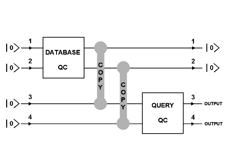
FIG. 3.: Structure of a quantum program for Grover’s search algorithm, using a 2-qubit QC to hold the database information and another 2-qubit QC to perform the search.

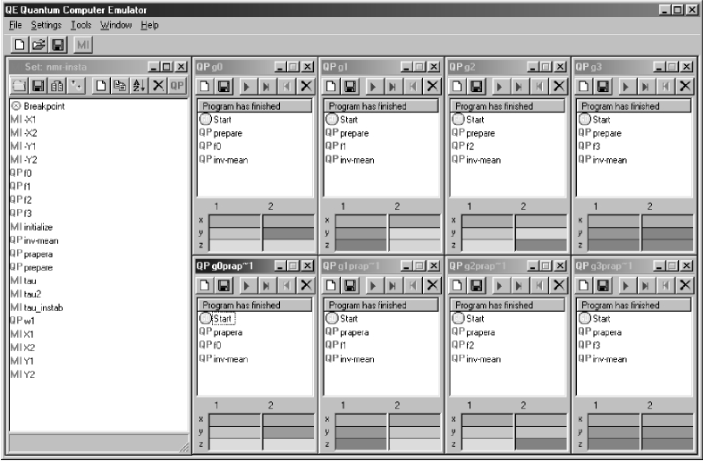
FIG. 4.: Snapshot of the Quantum Computer Emulator showing a window with a set of operations implementing a quantum computer using resonant pulses and windows with quantum programs implementing Grover’s database search.

REFERENCES

- [1] R. P. Feynman, Int. J. Theor. Phys. 21, 467 (1982).
- [2] D. P. DiVincenzo, Science 270, 255 (1995).
- [3] A. Ekert and R. Josza, Rev. Mod. Phys. 68, 733 (1996).
- [4] V. Vedral and M. B. Plenio, Prog. Quant. Electron. 22, 1 (1998).
- [5] D. Aharonov, e-print quant-ph/9812037 .
- [6] A. Ekert, Physica Scripta T76, 218 (1998).
- [7] P. W. Shor, in Proceedings of the 35th Annual Symposium on Foundations of Computer Science, edited by S. Goldwasser (IEEE Computer Society, Los Alamitos CA, 1994), p. 124.
- [8] I. L. Chuang, R. Laflamme, P. W. Shor, and W. Zurek, Science 270, 1633 (1995).
- [9] L. K. Grover, in Proceedings of the 28th Annual ACM Symposium of Theory of Computing (ACM, Philadelphia, 1996).
- [10] L. K. Grover, Phys. Rev. Lett. 79, 4709 (1997).
- [11] L. K. Grover, Phys. Rev. Lett. 80, 4329 (1998).
- [12] P. W. Shor, SIAM Rev. 41, 303 (1999), updated version. See Ref. [7].
- [13] J. Kim, J.-S. Lee, and S. Lee, Phys. Rev. A 61, 032312 (2000).
- [14] R. Gingrinch, C. Williams, and N. Cerf, Phys. Rev. A 61, 052313 (2000).
- [15] J. Jones and M. Mosca, J. of Chem. Phys. 109, 1648 (1998).
- [16] J. Jones, M. Mosca, and R. Hansen, Nature 393, 344 (1998).
- [17] I. L. Chuang, L. M. Vandersypen, X. Zhou, D. W. Leung, and S. Lloyd, Nature 393, 143 (1998).
- [18] I. L. Chuang, N. Gershenfeld, and M. Kubinec, Phys. Rev. Lett. 80, 3408 (1998).
- [19] R. Marx, A. Fahmy, J. Meyers, W. Bernel, and S. Glaser, e-print quant-ph/9905087 .
- [20] E. Knill, R. Laflamme, R. Martinez, and C.-H. Tseng, Nature 404, 368 (2000).
- [21] J. Cirac and P. Zoller, Phys. Rev. Lett. 74, 4091 (1995).
- [22] C. Monroe, D. Meekhof, B. King, W. Itano, and D. Wineland, Phys. Rev. Lett. 75, 4714 (1995).
- [23] T. Sleator and H. Weinfurter, Phys. Rev. Lett. 74, 4087 (1995).
- [24] P. Domokos, J. Raimond, M. Brune, and S. Haroche, Phys. Rev. A 52, 3554 (1995).
- [25] B. Kane, Nature 393, 133 (1998).
- [26] A. Imamog̃lo, D. Awschalom, G. Burkard, D. DiVincenzo, D. Loss, M. Sherwin, and A. Small, Phys. Rev. Lett. 83, 4204 (1999).
- [27] Y. Makhlin, G. Schön, and A. Shnirman, Nature 398, 305 (1999).
- [28] Y. Nakamura, Y. A. Pashkin, and J. S. Tsai, Nature 398, 786 (1999).
- [29] G. Nogues, A. Rauschenbeutel, S. Osnaghi, M. Brune, and J. Raimond, Nature 400, 239 (1999).
- [30] K. Molmer and A. Sorensen, Phys. Rev. Lett. 82, 1835 (1999).
- [31] A. Sorensen and K. Molmer, Phys. Rev. Lett. 82, 1971 (1999).
- [32] R. Fazio, G. M. Palma, and J. Siewert, Phys. Rev. Lett. 83, 5385 (1999).
- [33] T. Orlando, J. Mooij, L. Tian, C. H. van der Wal, L. Levitov, S. Lloyd, and J. Mazo, Phys. Rev. B 60, 15398 (1999).
- [34] A. Blias and Z. Zagoskin, Phys. Rev. A 61, 042308 (2000).
- [35] M. de Oliveira and W. Munro, Phys. Rev. A 61, 042309 (2000).
- [36] Download QCE from http://rugth30.phys.rug.nl/compphys/qce.htm. The examples presented in this paper are included in the software installation procedure.
- [37] H. De Raedt, A. Hams, K. Michielsen, and K. De Raedt, Comp. Phys. Comm. 132, 94 (2000).
- [38] H. De Raedt, A. Hams, K. Michielsen, S. Miyashita, and K. Saito, J. Phys. Soc. Jpn. Suppl. 69, 401 (2000).
- [39] C. Miquel, J. Paz, and W. Zurek, Phys. Rev. Lett. 78, 3871 (1995).
- [40] B. Pablo-Norman and M. Ruiz-Altaba, Phys. Rev. A 61, 012301 (2000).
- [41] G. L. Long, Y. S. Li, W. L. Zhand, and C. C. Tu, Phys. Rev. A 61, 042305 (2000).
- [42] G. P. Berman, G. D. Doolen, G. V. López, and V. I. Tsifrinovich, Phys. Rev. A 61, 062305 (2000).
- [43] G. P. Berman, G. D. Doolen, G. V. López, and V. I. Tsifrinovich, Phys. Rev. A 61, 042307 (2000).
- [44] S. Lloyd, Science 261, 1569 (1993).
- [45] G. P. Berman, G. D. Doolen, D. Holm, and V. I. Tsifrinovich, Phys. Lett. A 193, 444 (1994).
- [46] G. P. Berman, G. D. Doolen, R. Mainieri, and V. I. Tsifrinovich, Introduction to Quantum Computers (World Scientific, Singapore, 1998).
- [47] A. Barenco, C. H. Bennet, R. Cleve, D. P. DiVincenco, N. Margolus, P. Shor, T. Sleator, J. A. Smolin, and H. Weinfurter, Phys. Rev. A 52, 3457 (1995).
- [48] T. Cormen, C. Leiserson, and R. Rivest, Introduction to Algorithms (MIT Press, Cambridge, 1994).
- [49] J. Jones and M. Mosca, Phys. Rev. Lett. 83, 1050 (1999).
- [50] For numerical details download QCE.
- [51] S. Kak, Found. of Phys. 29, 267 (1999).
- [52] R. Ernst, G. Bodenhausen, and A. Wokaun, Principles of nuclear magnetic resonance in one and two dimensions (Claradon, Oxford, 1987).
- [53] R. Freeman, Spin Choreography (Spektrum Academic, Oxford, 1996).
- [54] C. Tseng, S. Somaroo, Y. Sharf, E. Knill, R. Laflamme, T. Havel, and D. Cory, Phys. Rev. A 61, 012302 (2000).
- [55] K. Doria, Arvind, and A. Kumar, Phys. Rev. A 61, 012302 (2000).
- [56] D. W. Leung, I. L. Chuang, F. Yamaguchi, and Y. Yamamoto, Phys. Rev. A 61, 042306 (2000).
- [57] K. Saito, S. Miyashita, and H. De Raedt, Phys. Rev. B 60, 14553 (1999).
- [58] S. Miyashita, K. Saito, H. Kobayshi, and H. De Raedt, J. Phys. Soc. Jpn. Suppl. 69, 395 .
- [59] R. Kubo, M. Toda, and N. Hashitsume, Statistical Physics II (Springer, New York, 1985).
- [60] K. Saito, S. Takesue, and S. Miyashita, Phys. Rev. E 61, 2397 (2000).
- [61] In terms of the NMR experiments referred to in this paper, this is an extremely low temperature.
- [62] G. D’Ariano and H. Yuen, Phys. Rev. Lett. 76, 2832 (1996).
- [63] C. Slichter, Principles of Magnetic Resonance (Springer, Berlin, 1990).
- [64] G. Baym, Lectures on Quantum Machanics (W.A. Benjamin, Reading MA, 1974).