Feedback-stabilization of an arbitrary pure state of a two-level atom

Abstract

Unit-efficiency homodyne detection of the resonance fluorescence of a two-level atom collapses the quantum state of the atom to a stochastically moving point on the Bloch sphere. Recently, Hofmann, Mahler, and Hess [Phys. Rev. A 57, 4877 (1998)] showed that by making part of the coherent driving proportional to the homodyne photocurrent can stabilize the state to any point on the bottom half of the sphere. Here we reanalyze their proposal using the technique of stochastic master equations, allowing their results to be generalized in two ways. First, we show that any point on the upper or lower half, but not the equator, of the sphere may be stabilized. Second, we consider non-unit-efficiency detection, and quantify the effectiveness of the feedback by calculating the maximal purity obtainable in any particular direction in Bloch space.

I Introduction

Although classical models of feedback schemes have been used for a long time to control dynamical noise, an analogous quantum theory of feedback has been developed only in the last fifteen years [1, 2, 3, 4, 5, 6, 7]. Recently there has been considerable interest in quantum feedback as a way to fight decoherence in isolated quantum systems, using the approach of Refs. [4, 5]. The central idea is to use a continuous measurement record, whose existence is due to the coupling of the system to a bath, to control the dynamics of the system so as to counteract the noise introduced by that bath and possibly other baths. For example, it has been suggested as a way to create optical squeezed states [8], to create micromaser number states [9], to correct errors in quantum bits [10], and to protect optical and microwave Schrödinger cat states against dissipation [11, 12, 13].

Decoherence in quantum systems can be loosely defined as loss of purity. Therefore the ultimate success in using feedback to fight decoherence would be to create an arbitrary stable pure state in the presence of dissipation. This goal was realized (better even that they realized) by Hoffman, Mahler and Hess (HMH) [14, 15] for a very simple system: a resonantly driven two-level atom. They showed that by using the photocurrent derived from unit-efficiency homodyne detection of the atom’s fluorescence to control part of the driving field of the atom, it is possible to exactly cancel the noise introduced by the electromagnetic vacuum field when the atom is in a particular pure state. By choosing the driving strength and feedback strength appropriately, any pure state on the Bloch sphere may be picked out, although HMH claimed that only pure states on the lower half of the sphere would be stable under their scheme.

HMH chose to describe detection and feedback in their system in a way different from (but equivalent to) the standard approach in Refs. [4, 5]. In this paper we reformulate their theory using the latter approach. This has the advantage of enabling a number of generalizations of their results. First, we revisit the question of stability and find that, contrary to the claims of HMH, the states in the upper half of the Bloch sphere can be stabilized as well as those in the lower half (this is what was better than they realized). The only states which cannot be stabilized, in the sense that an arbitrary initial state would not always end up in the desired state, are those on the equator of the Bloch sphere; that is, those which are equal superpositions of excited and ground states.

Our second generalization is to consider how effective feedback is with $\eta<1$; that is, with non-unit-efficiency detection. In this case it is not possible to stabilize the atom at any pure state, except the ground state which is trivially stable by setting the driving and feedback to zero. Instead, we aim to produce a steady state which is as close as possible to a given pure state. For the two-level atom, this is equivalent to trying to create a state which is as pure as possible in a particular direction in Bloch space. Not surprisingly (given the above result), we find that states near the equator cannot be well-protected against decoherence. We also find an echo of the distinction HMH found between the upper and lower halves of the Bloch sphere, in that states in the upper half sphere are affected much more by loss of detection efficiency that those in the lower half.

The paper is organized as follows. In Sec. II we present the model of a driven two-level atom, including the stochastic Schrödinger equation for unit-efficiency homodyne detection. In Sec. III we use this equation to derive the driving and feedback required to stabilize the atom in an arbitrary pure state. These results agree with those of HMH. However, our stability analysis disagrees substantially with theirs. In Sec. IV we present entirely new analytical results relating to the effect of non-unit- efficiency detection. In Sec. V we give numerical simulations of the stochastic evolution equations, illustrating the issues discussed in the preceding two sections. In Sec. VI we summarize and interpret our results, explain their significance, and discuss the possibility of future work.

II Homodyne Detection

A Master Equation

Consider a atom, with two relevant levels $\{|{g}\rangle,|{e}\rangle\}$ and lowering operator $\sigma=|{g}\rangle\langle{e}|$. Let the the decay rate be $\gamma$, and let it be driven by a resonant classical driving field with Rabi frequency $2\alpha$. This is as shown in Fig. 1, where for the moment we are omitting feedback by setting $\lambda=0$. This system is well-approximated by the master equation

$$\dot{\rho}=\gamma{\cal D}[\sigma]\rho-i\alpha[\sigma_{y},\rho],$$ (1)

where the Lindblad [16] superoperator is defined as usual ${\cal D}[A]B\equiv ABA^{\dagger}-\{A^{\dagger}A,B\}/2$. In this master equation we have chosen to define the $\sigma_{x}=\sigma+\sigma^{\dagger}$ and $\sigma_{y}=i\sigma-i\sigma^{\dagger}$ quadratures of the atomic dipole relative to the driving field. The effect of driving is to rotate the atom in Bloch space around the $y$-axis. The state of the atom in Bloch space is described by the three-vector $(x,y,z)$. It is related to the state matrix $\rho$ by

$$\rho=\frac{1}{2}\left({I+x\sigma_{x}+y\sigma_{y}+z\sigma_{z}}\right).$$ (2)

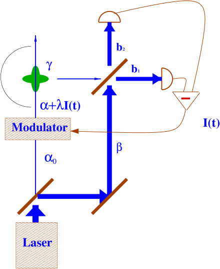
FIG. 1.: Diagram of the experimental apparatus. The laser beam is split to produce both the local oscillator $\beta$ and the field $\alpha_{0}$ which is modulated using the current $I(t)$. The modulated beam, with amplitude proportional to $\alpha+\lambda I(t)$, drives an atom at the centre of the parabolic mirror. The fluorescence thus collected is subject to homodyne detection using the local oscillator, and gives rise to the homodyne photocurrent $I(t)$.

It is easy to show that the stationary solution of the master equation (1) is

$${x}_{\rm ss} = \frac{4\alpha\gamma}{\gamma^{2}+8\alpha^{2}},$$ (3)

$${y}_{\rm ss} = 0,$$ (4)

$${z}_{\rm ss} = \frac{-\gamma^{2}}{\gamma^{2}+8\alpha^{2}}.$$ (5)

For $\gamma$ fixed, this is a family of solutions parameterized by the driving strength $\alpha\in(-\infty,\infty)$. All members of the family are in the $x$–$z$ plane on the Bloch sphere. Thus for this purpose we can reparametrize the relevant states using $r$ and $\theta$ by

$$x = r\sin\theta$$ (6)

$$z = r\cos\theta,$$ (7)

where $\theta\in[-\pi,\pi]$. Since

$${\rm Tr}[\rho^{2}]=\frac{1}{2}\left({1+x^{2}+y^{2}+z^{2}}\right)$$ (8)

is a measure of the purity of the Bloch sphere, $r=\sqrt{x^{2}+z^{2}}$, the distance from the centre of the sphere, is also a measure of purity. Pure states correspond to $r=1$ and maximally mixed states to $r=0$.

The locus of solutions in this plane (an ellipse) is shown in Fig. 2. Since $z_{\rm ss}<0$, all solutions are in the lower half of the Bloch sphere. That is, we are restricted to $|\theta|>\pi/2$. Also, it is evident that the smaller $|\theta|$ is (that is, the more excited the atom is), the smaller $r$ is (that is, the less pure the atom is). At $|\theta|=\pi$ the stationary state is pure, but this is not surprising as it is simply the ground state of the atom with no driving. As $|\theta|\to\pi/2$ we have $r\to 0$. This can only be approached asymptotically as $|\alpha|\to\infty$. In summary, the stationary states we can reach by driving the atom are limited, and generally far from pure.

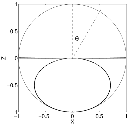
FIG. 2.: Locus of the solutions to the Bloch equations. The ellipse in the lower half plane is the locus for the equations with driving only. The full circle (minus the points on the equator) is the locus for the equations with optimal driving and feedback, as defined in Sec. III.

B Homodyne Detection

Now consider subjecting the atom to homodyne detection. As shown in Fig. 1, we assume that all of the fluorescence of the atom is collected and turned into a beam (represented in Fig. 1 by placing the atom at the focus of a mirror). Ignoring the vacuum fluctuations in the field, the annihilation operator for this beam is $\sqrt{\gamma}\sigma$, normalized so that the mean intensity $\gamma\left\langle{\sigma^{\dagger}\sigma}\right\rangle$ is equal to the number of photons per unit time in the beam. This beam then enters one port of a 50:50 beam splitter, while a strong local oscillator $\beta$ enters the other. To ensure that this local oscillator has a fixed phase relationship with the driving laser used in the measurement, it would be natural to utilize the same coherent light field source in the driving process and as the local oscillator in the homodyne detection. This is as shown in Fig. 1.

Again ignoring vacuum fluctuations, the two field operators exiting the beam splitter, $b_{1}$ and $b_{2}$, are

$$b_{k}=\left[{\sqrt{\gamma}\sigma-(-1)^{k}\beta}\right]/\sqrt{2}.$$ (9)

When these two fields are detected, the two photocurrents produced have means

$$\bar{I}_{k}=\left\langle{|\beta|^{2}-(-1)^{k}\left({\sqrt{\gamma}\beta\sigma^{\dagger}+\sqrt{\gamma}\sigma\beta^{*}}\right)+\gamma\sigma^{\dagger}\sigma}\right\rangle/2.$$ (10)

The middle two terms represent the interference between the system and the local oscillator.

The ideal limit of homodyne detection is when the local oscillator amplitude goes to infinity, which in practical terms means $|\beta|^{2}\gg\gamma$. In this limit, the rate of the photodetections goes to infinity and thus it should be possible to change the point process of photocounts into a continuous photocurrent with white noise. Also, the only relevant quantity is the difference between the two photocurrents. Suitably normalized, this is [17, 18]

$$I(t)=\frac{I_{1}(t)-I_{2}(t)}{|\beta|}=\sqrt{\gamma}\left\langle{e^{-i\Phi}\sigma^{\dagger}+e^{i\Phi}\sigma}\right\rangle_{\rm c}(t)+\xi(t).$$ (11)

A number of aspects of Eq. (11) need to be explained. First, $\Phi=\arg\beta$, the phase of the local oscillator (defined relative to the driving field). Second, the subscript c means conditioned and refers to the fact that if one is making a homodyne measurement then this yields information about the system. Hence, any system averages will be conditioned on the previous photocurrent record. Third, the final term $\xi(t)$ represents Gaussian white noise, so that

$$\xi(t)dt=dW(t),$$ (12)

an infinitesimal Wiener increment defined by [19]

$$dW(t)^{2}=dt,$$ (13)

$${\rm E}[dW(t)]=0.$$ (14)

Since the stationary solution of the master equation confines the state to the $x$–$z$ plane, it makes sense to follow HMH by setting $\Phi=0$. In that case,

$$I(t)=\sqrt{\gamma}\left\langle{\sigma_{x}}\right\rangle_{\rm c}(t)+\xi(t).$$ (15)

That is, the deterministic part of the homodyne photocurrent is proportional to $x_{\rm c}=\left\langle{\sigma_{x}}\right\rangle_{\rm c}$. This should be useful for controlling the dynamics of the state in the $x$–$z$ plane by feedback, as we will consider in Sec. III. Of course, all that really matters here is the relationship between the driving phase and the local oscillator phase, not the absolute phase of either.

The conditioning process referred to above can be made explicit by calculating how the system state changes in response to the measured photocurrent. Assuming that the state at some point in time is pure (which will tend to happen because of the conditioning anyway), its future evolution can be described by the stochastic Schrödinger equation (SSE) [17, 18]

$$d|{\psi_{\rm c}(t)}\rangle=\hat{A}_{\rm c}(t)|{\psi_{\rm c}(t)}\rangle dt+\hat{B}_{\rm c}(t)|{\psi_{\rm c}(t)}\rangle dW(t).$$ (16)

This is an Itô stochastic equation [19] with a drift term and a diffusion term. The operator for the drift term is

$$\hat{A}_{\rm c}(t)=\frac{\gamma}{2}\left[{-\sigma^{\dagger}\sigma+\left\langle{\sigma_{x}}\right\rangle_{\rm c}(t)\sigma-\left\langle{\sigma_{x}}\right\rangle_{\rm c}^{2}(t)/4}\right]-i\alpha\sigma_{y},$$ (17)

while that for the diffusion is

$$\hat{B}_{\rm c}(t)=\sqrt{\gamma}\left[{\sigma-\left\langle{\sigma_{x}}\right\rangle_{\rm c}(t)/2}\right].$$ (18)

Both of these operators are conditioned in that they depend on the system average

$$\left\langle{\sigma_{x}}\right\rangle_{\rm c}(t)=\langle{\psi_{\rm c}(t)}|\sigma_{x}|{\psi_{\rm c}(t)}\rangle.$$ (19)

On average, the system still obeys the master equation (1). This is easiest to see from the stochastic master equation (SME), which allows for impure initial conditions. The SME can be derived from the SSE by constructing

$$d\left({|{\psi_{\rm c}}\rangle\langle{\psi_{\rm c}}|}\right) = \left({d|{\psi_{\rm c}}\rangle}\right)\langle{\psi_{\rm c}}|+|{\psi_{\rm c}}\rangle\left({d\langle{\psi_{\rm c}}|}\right)$$ (21)

$${+}\,\left({d|{\psi_{\rm c}}\rangle}\right)\left({d\langle{\psi_{\rm c}}|}\right),$$

using the Itô rule (13), and then identifying $|{\psi_{\rm c}}\rangle\langle{\psi_{\rm c}}|$ with $\rho_{\rm c}$. The result is

$$d\rho_{\rm c}=dt\gamma{\cal D}[\sigma]\rho_{\rm c}-idt\alpha[\sigma_{y},\rho_{\rm c}]+dW(t)\sqrt{\gamma}{\cal H}[\sigma]\rho_{\rm c},$$ (22)

where ${\cal H}[A]B\equiv AB+BA^{\dagger}-{\rm Tr}[AB+BA^{\dagger}]$. Although this has been derived assuming pure initial conditions, it is valid for any initital conditions [18]. This is also an Itô equation, which means the evolution for the ensemble average state matrix

$$\rho(t)={\rm E}[\rho_{\rm c}(t)]$$ (23)

is found simply by averaging over the photocurrent noise term by using Eq. (14). This procedure yields the original master equation (1) again. The general term for the stochastic conditioned evolution of the system, be it described by a SSE or SME, is a quantum trajectory [17], and the quantum trajectory is said to unravel the master equation [17].

III Feedback with unit-efficiency detection

A SSE including feedback

We now include feedback onto the amplitude of the driving on the atom, proportional to the homodyne photocurrent, as done by HMH. This is as shown in Fig. 1, where the driving field passes through an electro-optic amplitude modulator controlled by the photocurrent, yielding a field proportional to $\alpha+\lambda I(t)$. This means that the feedback can be described by the Hamiltonian

$$H_{\rm fb}=\lambda\sigma_{y}I(t).$$ (24)

In this paper we are assuming instantaneous feedback, where the time delay in the feedback loop is negligible.

Since the homodyne photocurrent (11) is defined in terms of system averages and the noise $dW(t)$, the SSE including feedback can still be written as an equation of the form (16). The effect of the feedback Hamiltonian can be shown [4, 8] to change the drift and diffusion operators to

$$\hat{A}_{\rm c}(t) = \frac{\gamma}{2}\left[{-\sigma^{\dagger}\sigma+\left\langle{\sigma_{x}}\right\rangle_{\rm c}(t)\sigma-\left\langle{\sigma_{x}}\right\rangle_{\rm c}^{2}(t)/4}\right]-i\alpha\sigma_{y}$$ (26)

$${+}\,\lambda\sqrt{\gamma}\left[{-i\left\langle{\sigma_{x}}\right\rangle_{\rm c}(t)\sigma_{y}-2\sigma^{\dagger}\sigma}\right]-{\lambda^{2}}/{2},$$

$$\hat{B}_{\rm c}(t) = \sqrt{\gamma}\left[{\sigma-\left\langle{\sigma_{x}}\right\rangle_{\rm c}(t)/2}\right]-i\lambda\sigma_{y}.$$ (27)

Say we wish to stabilize the pure state with Bloch angle $\theta$, as defined in Eqs. (6) and (7), with $r=1$ of course. In terms of the ground and excited states, this state is

$$|{\theta}\rangle=\cos\frac{\theta}{2}|{e}\rangle+\sin\frac{\theta}{2}|{g}\rangle.$$ (28)

Now for this state to be stabilized we must have

$$\left[{\hat{A}_{\rm c}(t)dt+\hat{B}_{\rm c}(t)dW(t)}\right]|{\theta}\rangle\propto|{\theta}\rangle.$$ (29)

We cannot say the left-hand-side should equal zero because a change in the overall phase still leaves the physical state unchanged. However, we can work with this equation, and simplify it by dropping all terms proportional to the identity operator in $\hat{A}_{\rm c}(t)$ and $\hat{B}_{\rm c}(t)$. We can also demand that it be satisfied for the deterministic and noise terms separately, because $dW(t)$ can take any value. This gives the two equations

$$\left({\sqrt{\gamma}\sigma-i\lambda\sigma_{y}}\right)|{\theta}\rangle \propto |{\theta}\rangle,$$ (30)

$$\left[\gamma\left({-\sigma^{\dagger}\sigma+\sin\theta\sigma}\right)-i2\alpha\sigma_{y}\phantom{|{\sqrt{\gamma}}\rangle}\right.$$ (31)

$$\left.+\,\lambda\sqrt{\gamma}\left({-i\sin\theta\sigma_{y}/2-\sigma^{\dagger}\sigma}\right)\right]|{\theta}\rangle \propto |{\theta}\rangle,$$ (32)

where we have put $\left\langle{\sigma_{x}}\right\rangle_{\rm c}(t)$ equal to $\sin\theta$, its value for the state $|{\theta}\rangle$.

Solving the first equation easily yields the condition

$$\lambda=-\frac{\sqrt{\gamma}}{2}(1+\cos\theta).$$ (33)

This is equivalent to the feedback condition derived by HMH, stated as Eq. (35) of Ref. [15]. Substituting this into the second equation gives, after some trigonometric manipulation, the second condition

$$\alpha=\frac{\gamma}{4}\sin\theta\cos\theta.$$ (34)

Again, this agrees with the driving strength of HMH, given as Eq. (44) of Ref. [15]. It is worth emphasizing that the derivation given here is entirely different in detail from that of HMH, and so is an independent verification of their result. These functions are plotted in Fig. 3. Note that there are two points with the same values of both $\lambda$ and $\alpha$, at $\theta=\pm\pi/2$.

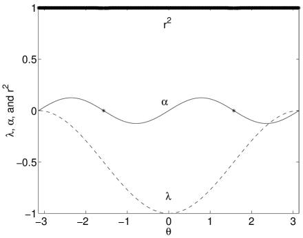
FIG. 3.: Plot of the optimal driving ($\alpha$, solid) and feedback ($\lambda$, dashed) required to produce a pure state with Bloch angle $\theta$. For this plot we have set $\gamma=1$ so that $\alpha$ and $\lambda$ are dimensionless. The purity ($r^{2}$, starred) is one except for $\theta=\pm\pi/2$, where the feedback is not stable.

B Stability

The preceding derivation seems to show that any pure state can be stabilized by a suitable choice of driving and feedback. Indeed our derivation proves that that if one prepares a state in exactly the pure state one desires, then the feedback scheme of HMH which we have analyzed will keep the system in that state. However, to discuss stability we need to know what will happen for states which are not initially in the desired state. To deal with this it is much more convenient to use the SME rather than the SSE, as will become apparent.

The SME can be constructed from the SSE in the same way as before. The result is [4, 8]

$$d\rho_{\rm c} = dt\gamma{\cal D}[\sigma]\rho_{\rm c}-idt\alpha[\sigma_{y},\rho_{\rm c}]$$ (37)

$${-}\,idt\lambda[\sigma_{y},\sigma\rho_{\rm c}+\rho_{\rm c}\sigma^{\dagger}]+dt(\lambda^{2}/\gamma){\cal D}[\sigma_{y}]\rho_{\rm c}$$

$${+}\,dW(t){\cal H}[\sqrt{\gamma}\sigma-i\lambda\sigma_{y}]\rho_{\rm c}.$$

Also as before, this is an Itô stochastic equation, which means that the ensemble average can be found simply by dropping the stochastic terms. This time, the result is not the original master equation, but rather the feedback-modified master equation

$$\dot{\rho}=-i[\alpha\sigma_{y},\rho]+{\cal D}[\sqrt{\gamma}\sigma-i\lambda\sigma_{y}]\rho\equiv{\cal L}\rho.$$ (38)

Here we have put the Liouvillian superoperator ${\cal L}$ in a manifestly Lindblad form.

Now we have shown already that the pure state $\rho=|{\theta}\rangle\langle{\theta}|$ must be a solution of this master equation, for the appropriate choices of $\lambda$ (33) and $\alpha$ (34). But for it to be a stable solution we require all of the eigenvalues of the resulting ${\cal L}_{\theta}$ to have a negative real part (except for the one eigenvalue that is always zero, as required for ${\cal L}_{\theta}$ to be norm-preserving). It is not difficult to find these eigenvalues, and in terms of $\theta$ they are

$$-{\gamma}/{2},-{\gamma}/{2},-\gamma\cos^{2}\theta.$$ (39)

Evidently the state $|{\theta}\rangle$ will be stable for all $\theta$ except $\theta=\pm\pi/2$. That is, all states are stable except those on the equator. This is contrary to the conclusion of HMH [15], based on a linearized stability analysis, that “long term stability of …inverted states [i.e. states in the upper half plane] cannot be achieved.” We emphasize that our stability analysis contains no approximations.

In hindsight, the lack of stability for pure states on the equator could have been predicted from the expressions (33) and (34). As discussed above and shown in Fig. 3, the values for driving and feedback for $\theta=\pi/2$ are the same as those for $\theta=-\pi/2$. This means that both $\rho=|{\pi/2}\rangle\langle{\pi/2}|$ and $\rho=|{-\pi/2}\rangle\langle{-\pi/2}|$ are solutions of ${\cal L}_{\theta}\rho=0$ for $\theta=\pi/2$ or $-\pi/2$. By linearity, any mixture of $|{\pi/2}\rangle\langle{\pi/2}|$ and $|{-\pi/2}\rangle\langle{-\pi/2}|$ will be a solution also. Hence any deviation away from one of these pure state will not necessarily be suppressed, and the system lacks stability. With random external perturbations, the system will eventually reach an equal mixture of $|{\pi/2}\rangle\langle{\pi/2}|$ and $|{-\pi/2}\rangle\langle{-\pi/2}|$, which is a state with $r=0$ (minimum purity). This is why we have plotted a value of $r=0$ in Fig. 3 for $|\theta|=\pi/2$. We also plot $r$ as a function of $\theta$ in Bloch space in Fig 2, giving the locus of states which can be stabilized by feedback. This can compared to the locus of the mixed states which are accessible by driving alone. We will return to the stability issue in the context of stochastic dynamics in Sec. V.

IV Feedback with non-unit-efficiency detection

We have seen that the stochastic master equation is a very useful representation of a quantum trajectory, as it allows the unconditioned (deterministic) master equation to be derived easily, and this latter equation is all that is required for a completely rigorous stability analysis. The SME is also superior to the SSE in that allows inefficient detection to be described. In a real experiment this has to be taken into account. The effect of non-unit $\eta$ on feedback in the present system is of interest both in itself, and because of the extreme nonlinearity of the system dynamics as compared to other quantum optical feedback systems such as considered in Ref. [8].

As explained in Ref. [18], the homodyne photocurrent from a detection scheme with efficiency $\eta$ is

$$I(t)=\sqrt{\gamma}\left\langle{\sigma_{x}}\right\rangle_{\rm c}(t)+\xi(t)/\sqrt{\eta}.$$ (40)

Here we have used a normalization such that the deterministic part does not depend on $\eta$. The effect of decreased efficiency is increased noise. This means that we can retain the same feedback Hamiltonian as above (24), without changing the significance of the feedback parameter $\lambda$. The SME with $\eta<1$, including feedback, is [8]

$$d\rho_{\rm c} = dt\gamma{\cal D}[\sigma]\rho_{\rm c}-idt\alpha[\sigma_{y},\rho_{\rm c}]$$ (43)

$${-}\,idt\lambda[\sigma_{y},\sigma\rho_{\rm c}+\rho_{\rm c}\sigma^{\dagger}]+dt(\lambda^{2}/\gamma\eta){\cal D}[\sigma_{y}]\rho_{\rm c}$$

$${+}\,dW(t){\cal H}[\sqrt{\gamma\eta}\sigma-i\lambda\sigma_{y}/\sqrt{\eta}]\rho_{\rm c}$$

The no-feedback SME, analogous to Eq. (22), can be obtained simply by setting $\lambda=0$, and was derived in Ref. [18].

Once again, it is easiest for the moment to just consider the ensemble average evolution by averaging $dW$ to zero. The Lindblad form of the resulting master equation is

$$\dot{\rho}=-i[\alpha\sigma_{y},\rho]+{\cal D}[\sqrt{\gamma}\sigma-i\lambda\sigma_{y}]\rho+(\lambda^{2}/\eta){\cal D}[\sigma_{y}]\rho.$$ (44)

We do not know a priori what values of $\lambda$ and $\alpha$ to choose to give the best results with inefficient detection, as the SSE analysis in Sec. III A obviously does not apply. Hence we simply solve for the stationary matrix in terms of $\alpha$ and $\lambda$. Using the Bloch representation we find

$${x}_{\rm ss} = {4\alpha\eta^{2}(\gamma+2\sqrt{\gamma}\lambda)}/D,$$ (45)

$${y}_{\rm ss} = 0,$$ (46)

$${z}_{\rm ss} = -\sqrt{\gamma}\eta(\sqrt{\gamma}+2\lambda)(\gamma\eta+4\sqrt{\gamma}\eta\lambda+4\lambda^{2})/D,$$ (47)

where

$$D = \gamma^{2}\eta^{2}+6\gamma^{3/2}\eta^{2}\lambda+2\gamma\eta(3+4\eta)\lambda^{2}+16\sqrt{\gamma}\eta\lambda^{3}$$ (49)

$${+}\,8(\alpha^{2}\eta^{2}+\lambda^{4}).$$

The question now arises, what do we mean by “best results” for the feedback system. We cannot hope anymore to produce stable pure states anywhere on the Bloch sphere. However, we can pick a direction $\theta$ on the Bloch sphere and ask how close can we get to a pure state? That is, we use the radius $r$ in Eq. (6) and Eq. (7) as the quantity to be maximized, for each $\theta$. From these two equations we have

$$\tan\theta=x_{\rm ss}/z_{\rm ss}.$$ (50)

¿From Eqs. (45) and (47) we can immediately find the desired driving in terms of $\lambda$ and $\theta$ as

$$\alpha=\frac{-\sqrt{\gamma}\eta(\sqrt{\gamma}+2\lambda)(\gamma\eta+4\sqrt{\gamma}\eta\lambda+4\lambda^{2})\tan\theta}{4\eta^{2}(\gamma+2\sqrt{\gamma}\lambda)}.$$ (51)

The aim is then, for each $\theta$, to find the feedback $\lambda$ which maximizes

$$r^{2}=x_{\rm ss}^{2}+z_{\rm ss}^{2}.$$ (52)

This was done numerically using matlab.

The results of our calculations are shown in Fig. 4, where we plot the locus in Bloch space of the best (most pure) stationary states which can be achieved by feedback from non-unit-efficiency detection. We use a variety of values of $\eta$. A number of points are worth noting. First, and most obviously, the degree of purity (measured by the $r$, the distance from the origin) decreases with $\eta$. Second, the gap at the equator for $\eta=1$ quickly widens, so that the purity of the best states with $\theta$ close to $\pi/2$ is small. Third, the purity of the best states in the upper half of the Bloch sphere is affected much more by loss of detection efficiency than those in the lower half. Fourth, in the limit $\eta=0$, the best solutions correspond to the no-feedback solutions shown in Fig. 2. This is not surprising, since with $\eta=0$ the photocurrent contains no information about the system (as the noise is infinitely large) and hence there is no point doing feedback. Since the stationary states with no feedback are confined to the lower half of the Bloch sphere, this explains why the best states with feedback in the lower half are less affected as $\eta$ decreases than those in the upper half.

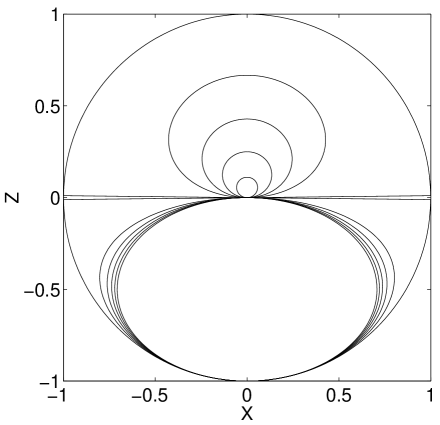
FIG. 4.: Locus of the solutions to the Bloch equations with optimal feedback for different values of detector efficiency $\eta$. from the outside in, we have $\eta=1,0.8,0.6,0.4,0.2,0$.

For the particular value $\eta=0.8$ we plot in Fig. 5 the values of $\alpha$ and $\lambda$ (as well as purity, quantified as $r^{2}$) versus $\theta$. By comparing this plot with Fig. 3 one obtains some idea of the effect of inefficient detection. A number of features remain the same. First, $\alpha$ is antisymmetric in $\theta$, while $\lambda$ is symmetric. Recalling that the deterministic part of the feedback is proportional to $\lambda\left\langle{\sigma_{x}}\right\rangle_{\rm c}$, the feedback itself is actually antisymmetric as well as the driving. Second, the magnitude of the feedback is zero for $|\theta|=\pi$ (the ground state) and increases monotonically to a maximum of $\sqrt{\gamma}$ at $\theta=0$ (in the direction of the excited state). Third, the driving is zero at the ground state and at $\theta=0$, and also changes sign as one passes through the equatorial place. The most obvious difference between the parameters for $\eta=1$ and those for $\eta=0.8$ parameter is that the latter have a discontinuity at $|\theta|=\pi/2$. The feedback parameter $\lambda$ jumps as one crosses the equatorial plane, while the driving $\alpha$ asymptotes to $+\infty$ on one side and $-\infty$ on the other. These extreme variations in the driving do not prevent the best purity from approaching zero in the equatorial plane.

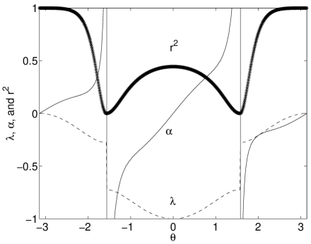
FIG. 5.: Plot of the optimal driving ($\alpha$, solid) and feedback ($\lambda$, dashed) required to produce the most pure state with Bloch angle $\theta$. For this plot we have set $\gamma=1$ so that $\alpha$ and $\lambda$ are dimensionless. The purity obtain is also plotted ($r^{2}$, starred).

V Stochastic Dynamics

A Stochastic Bloch Equations

So far we have considered the stochastic conditioned dynamics for the system state in order to derive the parameters $\lambda$ and $\alpha$ such that for $\eta=1$ those dynamics are banished in the steady state. In this section we will consider them in more detail, highlighting the difference between the $\eta=1$ case and the $\eta<1$ case, and also looking in more detail at the special case of $|\theta|=\pi/2$. The most convenient way to treat the stochastic dynamics in general is through the stochastic Bloch equations (SBE). These are simply the stochastic equations for the conditioned Bloch vector, defined by

$$\rho_{\rm c}=\frac{1}{2}\left({I+x_{\rm c}\sigma_{x}+y_{\rm c}\sigma_{y}+z_{\rm c}\sigma_{z}}\right).$$ (53)

¿From the SME including feedback (43), we find

$$\left(\begin{array}[]{c}dx_{\rm c}\\ dy_{\rm c}\\ dz_{\rm c}\end{array}\right) = dt\left(\begin{array}[]{ccc}-\gamma/2-2\kappa&0&2\alpha\\ 0&-{\gamma}/{2}&0\\ -2\alpha&0&-\gamma-2\kappa\\ \end{array}\right)\left(\begin{array}[]{c}x_{\rm c}\\ y_{\rm c}\\ z_{\rm c}\end{array}\right)$$ (71)

$${-}\,dt\left(\begin{array}[]{c}0\\ 0\\ 2\lambda\sqrt{\gamma}+\gamma\end{array}\right)+dW(t)\times$$

$$\left(\begin{array}[]{c}-\sqrt{\gamma\eta}x_{\rm c}^{2}+(\sqrt{\gamma\eta}+{2\lambda}/{\sqrt{\eta}})z_{\rm c}+\sqrt{\gamma\eta}\\ -\sqrt{\gamma\eta}x_{\rm c}y_{\rm c}\\ -(\sqrt{\gamma\eta}+{2\lambda}/{\sqrt{\eta}})x_{\rm c}-\sqrt{\gamma\eta}x_{\rm c}z_{\rm c}\end{array}\right),$$

where $\kappa={\lambda^{2}}/{\eta}+\lambda\sqrt{\gamma}$. If we ignore the final (noise) term, we get the Bloch equations from the master equation (44).

B unit-Efficiency

In the case $\eta=1$, considered in Sec. III, both the deterministic and stochastic dynamics disappeared in the steady state for the appropriate choice of $\alpha$ and $\lambda$. Because the stationary solution of the SSE was a unique pure state, that was necessarily also the stationary solution of the master equation found by averaging over the noise in the equivalent SME. Thus there was no distinction between the unconditioned and conditioned states. There are two exceptions to this lack of distinction. The first is in the transients, before the system reaches its steady state. The second is for the special case $|\theta|=\pi/2$. In this subsection we investigate these exceptions.

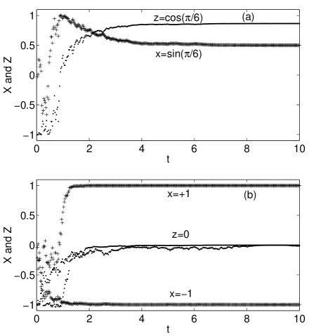
FIG. 6.: Typical quantum trajectories for optimal feedback with $\eta=1$, shown by $x_{\rm c}$ (plusses) and $z_{\rm c}$ (dots) as functions of time. (a) shows a single trajectory for $\theta=\pi/6$, and (b) two trajectories for $\theta=\pi/2$.

First, the transient behaviour was simulated using the SBE with $\eta=1$. We chose the initial state to be the ground state, and evolved the system stochastically from $t=0$ to $t=10\gamma^{-1}$. With this choice of initial condition, $y_{\rm c}=0$ for all time. We verified that in each trajectory $x_{\rm c}^{2}+z_{\rm c}^{2}=1$ to a good approximation (indicating a pure state), but that the ensemble averages over many trajectories

$$x={\rm E}[x_{\rm c}]\;,\;\;z={\rm E}[z_{\rm c}]$$ (73)

obey the deterministic Bloch equations. A typical trajectory for $\theta=\pi/6$ is shown in Fig. 6(a). We see that the initial evolution is very erratic, but that on a time scale of a few $\gamma^{-1}$ the system relaxes towards a steady state which is pure and stationary. By $t=10\gamma^{-1}$ the system is locked in a stable pure state for all intents. We have also illustrated another typical trajectory in Bloch space, in Fig. 7.

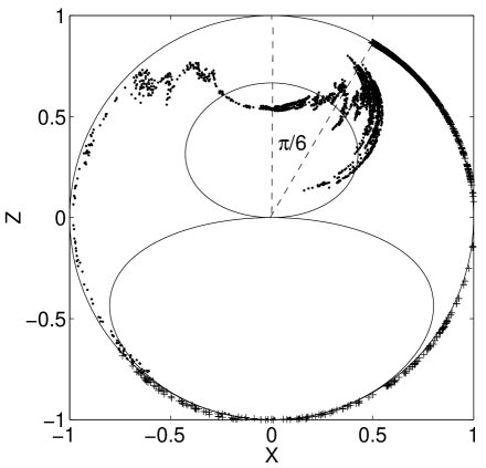
FIG. 7.: Typical quantum trajectories in Bloch space for $t\in[0,10\gamma^{-1}]$ under optimal feedback for $\theta=\pi/6$, starting at the ground state. The plusses are for $\eta=1$ and the dots for $\eta=0.8$. The locus for the deterministic stationary states for $\eta=0.8$ are also shown; the relevant state for this quantum trajectory is at the intersection of the locus and the ray at $\theta=\pi/6$. Note that the quantum trajectory for $\eta=0.8$ wanders around this average position, while that for $\eta=1$ stops precisely at the desired pure steady state.

It is easy to verify that by putting $\eta=1$ and

$$(x_{\rm c},y_{\rm c},z_{\rm c})=(\sin\theta,0,\cos\theta)$$ (74)

in the right-hand-side of the SBE (LABEL:SBE1), we obtain complete cancellation. If we wish, we can follow HMH and separate the noise term into the contribution from feedback (proportional to $\lambda$) and that contribution present even without feedback (the rest). We interpret the latter stochasticity as being due to the quantum measurement we are making, with its underlying probabilistic nature. Obviously the fluctuation due to measurement is canceled by the feedback, as HMH point out. It is equally important that the deterministic dynamics are also canceled at this point.

The story for the special case $\theta=\pi/2$ is quite different. For this case the SBEs are

$$\left(\begin{array}[]{c}dx_{\rm c}\\ dy_{\rm c}\\ dz_{\rm c}\end{array}\right) = dt\left(\begin{array}[]{ccc}0&0&0\\ 0&-{\gamma}/{2}&0\\ 0&0&-\gamma/2\\ \end{array}\right)\left(\begin{array}[]{c}x_{\rm c}\\ y_{\rm c}\\ z_{\rm c}\end{array}\right)$$ (88)

$${+}\,\sqrt{\gamma}dW(t)\left(\begin{array}[]{c}1-x_{\rm c}^{2}\\ -x_{\rm c}y_{\rm c}\\ -x_{\rm c}z_{\rm c}\end{array}\right).$$

Here the three eigenvalues in Eq. (39) are clearly evident. Both $z_{c}$ and $y_{\rm c}$ will decay to zero (as required for $\theta=\pi/2$), and their noise terms vanish at that point. By contrast, the equation for $x_{\rm c}$ is independent of the others, and is purely stochastic:

$$dx_{\rm c}=\sqrt{\gamma}dW(t)(1-x_{\rm c}^{2}).$$ (89)

Clearly the equatorial pure states with $x_{\rm c}=\pm 1$ are stationary solutions to this problem. Also, the system will tend to one of these states. We can see this by calculating

$$d{\rm E}[x_{\rm c}^{2}]=\gamma dt{\rm E}\left[{(1-x_{\rm c}^{2})^{2}}\right],$$ (90)

which is always positive. That is, on average $x_{\rm c}^{2}$ always increases. But it is also clear that $x_{\rm c}$ has no preference to go to either of these states. Hence they are not stable. The ensemble average $x$ is unchanging under this evolution. Thus a perturbation which moves the state from $x_{\rm c}=1$ to $x_{\rm c}=1-\epsilon$ say, will result in a proportion $\epsilon/2$ of the states ending up at $x_{\rm c}=-1$, and a proportion $1-\epsilon/2$ ending up at $x_{\rm c}=1$.

We have illustrated these features by showing two typical trajectories in Fig. 6(b). Once again, the initial evolution is highly erratic, but the system reaches a fixed point on a time scale of a few $\gamma^{-1}$. However, with the same initial condition (the ground state), one trajectory ends up at $x_{\rm c}=1$ and the other at $x_{\rm c}=-1$.

C Non-unit-efficiency

In the unit-efficiency case the stationary solution of the master equation is (except for $|\theta|=\pi/2$), a pure state. This is very special in that in means that every unraveling of the master equation as a SSE or SME must end up in this same pure state also. For non-unit-efficiency we have found the most pure stable state for each $\theta$. In this case we must use a SME to unravel the master equation, since the conditioned state will not be pure in general, because of the inefficient detection. Since the deterministic steady state is not pure (except for $|\theta|=\pi$), the quantum trajectories need not end up in this state. Instead, the quantum state in an individual trajectory may continue to evolve stochastically even when the system is in steady state, and the equivalence to the deterministic evolution may hold only on average. On the other hand, it is also possible that the quantum trajectories do all end up in the deterministic steady state, since we expect the conditioned state to be mixed anyway.

It turns out that with the optimal values of $\alpha$ and $\lambda$ defined in Sec. IV, the actual behaviour is the first option described above. That is, the system state continues to vary stochastically in the long time limit, but is constrained so that the time-averaged state is equal to the solution of the deterministic master equation. We show this in Bloch space Fig. 7 for $\eta=0.8$ and $\theta=\pi/6$. We see that the amount of randomness in the system state in the long-time limit is quite large even for fairly high $\eta$.

This result suggests another question: would a different choice for $\lambda$ be able to reduce, or even eliminate, the randomness in the steady-state quantum trajectory, even though it would necessarily be at the expense of the purity of the deterministic stationary solution. [Recall that for a given $\lambda$, $\alpha$ is still necessarily fixed by Eq. (51).] To test this idea we tried choosing $\lambda$ based not on maximizing $r^{2}$ as in Eq. (52), but on minimizing

$$N_{\theta}(\lambda)=\left|\left(\begin{array}[]{c}-\sqrt{\gamma\eta}x_{\rm ss}^{2}+(\sqrt{\gamma\eta}+{2\lambda}/{\sqrt{\eta}})z_{\rm ss}+\sqrt{\gamma\eta}\\ -\sqrt{\gamma\eta}x_{\rm ss}y_{\rm ss}\\ -(\sqrt{\gamma\eta}+{2\lambda}/{\sqrt{\eta}})x_{\rm ss}-\sqrt{\gamma\eta}x_{\rm ss}z_{\rm ss}\end{array}\right)\right|^{2}.$$ (91)

That is, we minimize the noise terms in the SBE Eq. (LABEL:SBE1). Note that we have replaced the conditioned Bloch variables $x_{\rm c}$ etc. with the deterministic stationary solutions $x_{\rm ss}$ etc., and that the dependence of these stationary solutions on $\alpha$ and $\lambda$ add a further, implicit, dependence on $\lambda$ to $N_{\theta}(\lambda)$. This is a sensible procedure if the aim is realizable, and the noise in the solutions is reduced or eliminated so that the conditioned states are approximately or exactly equal to the deterministic stationary solution.

It turns out that this procedure cannot significantly reduce the amount of steady-state randomness in the quantum trajectories below that resulting from minimizing the deterministic stationary purity. In fact, for all values of $\eta$ we considered, the variation of $\lambda$ (as a function of $\theta$) based on minimizing the noise was indistinguishable by eye from that based on maximizing the purity. This is not too surprising, but could not have been predicted a priori.

VI Conclusion

We have given a rigorous analysis of the anti-decoherence feedback scheme proposed by Hofmann, Mahler and Hess [15]. They proposed modulating the driving of a two-level atom using the instantaneous homodyne photocurrent, in order to stabilize the atom in an arbitrary known pure state. We have shown that, for detection efficiency $\eta=1$, the pure states thus produced are stable. This is contrary to the conclusion of HMH, that only pure states in the lower half of the Bloch sphere would be stable. The one exception we found is for pure states on the equator. Although they are fixed points of the dynamics, they are not stable. A small perturbation away from one fixed pure state leads to a proportionally small fraction of the ensemble ending up in the diametrically opposite pure state.

It is nevertheless possible to obtain an asymmetry between the upper and lower halves of the Bloch sphere, reminiscent of the conclusion of HMH, if one considers detection efficiencies less than one. In this case, it is no longer possible to stabilize the system in a given pure state, so we choose the feedback and driving so that the solution of the master equation (including feedback) is as close as possible to a given pure state. We find that the purity (which measures this closeness) of states thus produced decays to zero as $\eta$ decreases to zero, for states in the upper half of the Bloch sphere. By contrast, those in the lower half do not decay to zero. This is readily understandable since in the absence of feedback (which is the situation which must prevail when the detection efficiency goes to zero), the master equation with driving alone has stationary solutions in the lower-half plane with non-zero purity. The purity decays most rapidly with $\eta$ for states near the equator, which is unsurprising given the instability of states on the equator even for $\eta=1$.

In the non-unit-efficiency case, the state of the system conditioned on the homodyne measurement results continues to evolve stochastically even in the long-time limit, where the ensemble average evolution has reached the desired most-pure state. Moreover, it seems that any other choice of driving and feedback will result in more, not less, randomness in the steady-state quantum trajectory.

Our results are significant in a number of ways. First, they show the power of the quantum trajectory and master equation techniques developed in Refs. [4, 8, 5]. Those techniques were particularly useful for illuminating subtle questions regarding the stability of pure states, and for treating inefficient detection. Second, the physical system (the two-level atom) may one day find application as a quantum bit in quantum information technology [20]. In that eventuality, the ability to stabilize the atom against dissipation in an arbitrary (known) pure state may be useful. Third, the system is a simple but non-trivial example of quantum feedback in a nonlinear system (the two-level atom). Thus the effectiveness of feedback, and in particular the influence of non-unit- efficiency detection on this effectiveness, is of interest for what it may tell us about other more complicated nonlinear systems.

In this last context, it would be of interest to also consider the effect of non-Markovian feedback; that is, feedback with a time delay or non-flat loop response function. This is much more difficult to treat than Markovian feedback because the Lindblad master equations derived in Refs. [4, 8, 5] do not apply. Analytical solutions for non-Markovian feedback are possible for linear systems [8, 21]. For a nonlinear system like the two-level atom, numerical simulations, or novel analytical approaches, are necessary. This is an issue we plan to explore in future work.

REFERENCES

- [1] H. A. Haus and Y. Yamamoto, Phys. Rev. A 34, 270 (1986).
- [2] Y. Yamamoto, N. Imoto and S. Machida, Phys. Rev. A 33, 3243 (1986).
- [3] J. M. Shapiro et al, J. Opt. Soc. Am. B 4, 1604 (1987).
- [4] H. M. Wiseman and G. J. Milburn, Phys. Rev. Lett. 70, 548 (1993).
- [5] H. M. Wiseman, Phys. Rev. A 49, 2133 (1994).
- [6] L. Plimak, Phys. Rev. A 50, 2120 (1994).
- [7] A.C. Doherty and K. Jacobs, Phys. Rev. A 60, 2700 (1999).
- [8] H.M. Wiseman and G.J. Milburn, Phys. Rev. A 49, 1350 (1994).
- [9] A. Liebman and G.J. Milburn, Phys. Rev. A 51, 736 (1995).
- [10] H. Mabuchi and P. Zoller, Phys. Rev. Lett. 76, 3108 (1996).
- [11] P. Tombesi and D. Vitali, Phys. Rev. A 50, 4253 (1994).
- [12] D. B. Horoshko and S. Ya. Kilin, Phys. Rev. Lett. 97, 840 (1997).
- [13] D. Vitali, P. Tombesi, and G.J. Milburn, Phys. Rev. Lett. 79, 2442 (1997).
- [14] H. F. Hofmann, O. Hess, and G. Mahler, Optics Express 2, 339 (1998).
- [15] H. F. Hofmann, G. Mahler, and O. Hess, Phys. Rev. A, 57, 4877 1998.
- [16] G. Lindblad, Commun. Math. Phys. 48, 199 (1976).
- [17] H.J. Carmichael, An Open Systems Approach to Quantum Optics (Springer-Verlag, Berlin, 1993).
- [18] H.M. Wiseman and G.J. Milburn, Phys. Rev. A 47, 642 (1993).
- [19] C.W. Gardiner, Handbook of Stochastic Methods (Springer, Berlin, 1985).
- [20] C.P. Williams and S.H. Clearwater, Explorations in Quantum Computing (Springer, New York, 1998).
- [21] V. Giovannetti, P.Tombesi, and D.Vitali, Phys. Rev. A, 60, 1549 (1999).