Cooling of a single atom in an optical trap inside a resonator

Abstract

We present detailed discussions of cooling and trapping mechanisms for an atom in an optical trap inside an optical cavity, as relevant to recent experiments. The interference pattern of cavity QED and trapping fields in space makes the trapping wells in principle distinguishable from one another. This adds considerable flexibility to creating effective trapping and cooling conditions and to detection possibilities. Friction and diffusion coefficients are calculated in and beyond the low excitation limit and full 3-D simulations of the quasiclassical motion of a Cs atom are performed.

32.80.Pj, 42.50.Vk, 42.50.Lc

I Introduction

A recent experiment [1] succeeded in trapping a single atom with single photons inside an optical cavity and in monitoring the atomic motion with the resolution approaching the standard quantum limit for position measurements. Yet a second experiment [2] has likewise reported single-atom trapping at the few-photon level, although in this case the trapping potential and diffusion are in fact well approximated by a free-space semiclassical theory [3].

One future objective for such experiments is to use atoms trapped in cavities for quantum communication purposes, with atoms serving as quantum memories and photons as the transporters of quantum information [4, 5]. While the single-photon trapping experiments provide a new paradigm for quantum measurement and control, they are nevertheless not entirely suitable for the purpose of distributed quantum networks where qubits will be communicated among quantum nodes. The reason is the short trapping life time of the atoms as well as limited operation flexibility. A better strategy might be to use the cavity QED field for quantum state entanglement and distribution while an additional (external) trapping mechanism provides the necessary confinement of the atomic center-of-mass motion. For instance, in another recent experiment from the Caltech group [6], mean trapping times of $\sim 28$ms (as compared to mean trapping times of $<1$msec in the experiments [1, 2]) were achieved by employing a far-off resonant trapping (FORT) beam along the cavity axis. In that experiment the trapping lifetime was limited due to intensity fluctuations of the intracavity FORT beam [7]. Here we consider the situation of current improved experiments [8] in which a single atom is held inside an optical cavity in a stable FORT beam of minimum intensity fluctuations.

Several mechanisms for cooling inside optical resonators have been discussed before [9, 10, 11]. Here we discuss in detail how the combination of an external trapping potential and the cavity QED field adds flexibility in predetermining where and to what degree atoms will be trapped and cooled. Moreover, our calculations go beyond the weak driving limit discussed in [10]. That is, we allow the “probe” field driving the cavity to be so strong as to appreciably modify the dynamical behavior of, rather than merely probe, the atom-cavity system.

This paper is organized as follows. In Section II we describe the physical situation of an atom trapped in an optical potential and strongly interacting with a cavity QED field. We give the evolution equations for both internal and external atomic degrees of freedom and for the quantized cavity mode. Section III contains an exposition on how we calculated friction and diffusion coefficients from the forces acting on the atom. Section IV contains the main results of this paper: we discuss simple pictures for cooling mechanisms, based on the dressed state structure of the atom-cavity system, and give numerical results for the typical cooling and diffusion rates, and hence “temperatures” for single atoms under various trapping conditions. We also study the saturation behavior under strong driving conditions and perform simulations of the full 3-D motion of atoms trapped in particular wells that show how the probe field transmission is correlated with the atomic motion and how trapping times can be prolonged by strong cooling. Section IV F concludes with a brief discussion of a slightly different trapping scheme. The summary highlights the main results.

II Description of problem

We consider a single two-level atom coupled to a single quantized cavity mode and coupled to a (classical) far-off resonant trapping (FORT) beam. In most of the paper we assume that the FORT shifts the atomic excited state $|e\rangle$ up and the ground state $|g\rangle$ down by an amount $S_{F}(\vec{r})$ (i.e., the energy of the ground state is $E_{g}-S_{F}$, that of the excited state $E_{e}+S_{F}$), as this is the situation pursued in previous and current experiments [6, 8]. In Section IV F, however, we will also study the different situation where both ground and excited states are shifted down by $S_{F}$ (see e.g. [12]). The FORT beam coincides with one of the longitudinal modes of the cavity and its wavelength $\lambda_{F}$ is longer than that of the main cavity mode of interest for cavity QED, $\lambda_{0}$. In fact, in the experiments [6, 8] the cavity length $L$ is $104\lambda_{0}/2=102\lambda_{F}/2$.

The position-dependent AC-Stark shift due to the FORT field is of the form

$$S_{F}(\vec{r})=S_{0}\sin^{2}(k_{F}z)\exp(-2\rho^{2}/w_{0}^{2}),$$ (1)

with $S_{0}>0$ the maximum shift, $k_{F}=2\pi/\lambda_{F}$ the wave vector of the FORT field, $w_{0}$ the size of the Gaussian mode of the cavity, while $z$ and $\rho$ give the coordinate along, and the distance perpendicular to, the cavity axis, respectively. The quantized cavity mode is assumed to have the same transverse dimensions $w_{0}$ so that the atom-cavity coupling is determined by

$$g(\vec{r})=g_{0}\sin(kz)\exp(-\rho^{2}/w_{0}^{2}),$$ (2)

with $g_{0}$ the maximum coupling rate and $k=2\pi/\lambda_{0}$ the wave vector of the cavity mode. Under conditions where the cavity is not driven too strongly, the atom will be trapped around the anti-nodes of the red-detuned FORT field. Thanks to the fact that $\lambda_{0}\neq\lambda_{F}$, the atom will experience a different coupling strength to the cavity mode in each different well. Figure 1 shows the axial pattern arising from the FORT and cavity fields. For illustrative purposes we choose here (and in the rest of this paper) a cavity of length $L=16\lambda_{0}=15\lambda_{F}$. This does not influence the basic physics involved: in particular we note that the precise value of $\lambda_{F}$ is largely irrelevant on the time scales considered here, as the FORT field is detuned far from atomic resonance. The choice of $L=16\lambda_{0}=15\lambda_{F}$ just means that only 8 wells out of 30 are qualitatively and quantitatively different.

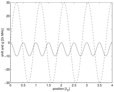
FIG. 1.: The FORT-induced shift of the ground state on axis ($\rho=0$) in the case where $S_{0}/(2\pi)=10$MHz and the cavity-QED coupling rate $g$ (dashed curve), with $g_{0}=3S_{0}$, as functions of position along the cavity axis measured in units of the FORT wavelength $\lambda_{F}$, with $z=0$ at the left cavity boundary. The cavity length is $L=15\lambda_{F}$.

This is illustrated in Fig. 2 where we plot the value of the cavity QED coupling $g$ at the anti-nodes of the FORT (i.e., the bottom of the trapping potential). In particular, there are 2 anti-nodes in which $g=0$, and 4 in which $|g|$ attains it maximum.

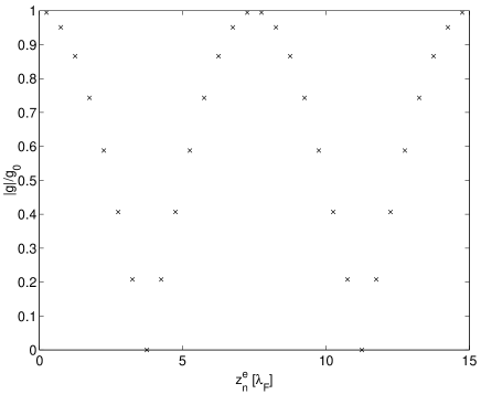
FIG. 2.: The values of $|g|/g_{0}$ at the locations of the anti-nodes of the FORT, i.e. at the points $z_{n}=(n/2-1/4)\lambda_{F}$ for $n=1\ldots 30$. There are 8 quantitatively different wells.

The cavity is driven by an external classical field ${\cal E}(t)={\cal E}_{0}\exp(i\omega_{p}t)$, at a frequency $\omega_{p}$, which is used to probe the atom-cavity system and which may cool the atom at the same time. In the following, the strength of the driving field is indicated by the number of cavity photons $N_{e}$ that would be present if there were no atom in the cavity, rather than by ${\cal E}_{0}$. This closely follows the experimental procedure for determining the driving strength. The relation between the two is

$$N_{e}=\frac{{\cal E}_{0}^{2}}{\kappa^{2}+\Delta_{c}^{2}},$$ (3)

with $\Delta_{c}=\omega_{c}-\omega_{p}$ the detuning of the probe from the cavity frequency $\omega_{c}=kc$. The Hamiltonian for the internal atomic degrees of freedom and the quantized cavity mode is, in a frame rotating at the probe frequency $\omega_{p}$, given by

$$H = \hbar\Delta_{c}a^{+}a+\hbar\Delta_{a}\sigma^{+}\sigma^{-}+2\hbar S_{F}(\vec{r})(\sigma^{+}\sigma^{-}-1/2)$$ (5)

$$+\hbar{\cal E}_{0}(a^{+}+a)+\hbar g(\vec{r})(a^{+}\sigma^{-}+\sigma^{+}a).$$

Here $\Delta_{a}=\omega_{a}-\omega_{p}$ is the detuning of the atomic resonance from the probe frequency. In all numerical examples given below the cavity frequency is chosen to coincide with the atomic frequency, so that $\Delta_{c}=\Delta_{a}$. The quantity $\Delta_{p}\equiv-\Delta_{a}$ is then referred to as the probe detuning. Note here that without a FORT the optimum cavity and atom detunings are not equal [9, 10, 11]. In our case, however, the FORT effectively changes the atomic frequency in a position-dependent way and thus the precise value of the atomic detuning relative to the cavity detuning is largely irrelevant. Indeed optimum cooling conditions will exist in certain wells but not in others, which is one feature that allows one to distinguish various wells.

Coupling the atom and the cavity to the remaining modes of the electro-magnetic field leads by a standard procedure to the master equation for the density operator of the coupled atom-cavity system,

$$\frac{{\rm d}\rho}{{\rm d}t}=-i[H,\rho]/\hbar-\kappa\{a^{+}a,\rho\}+2\kappa a\rho a^{+}+$$ (6)

$$-\frac{\Gamma}{2}\{\sigma^{+}\sigma^{-},\rho\}+\frac{3\Gamma}{8\pi}\int{\rm d}^{2}\hat{k}\sum_{\hat{\epsilon}}(\hat{d}\cdot\hat{\epsilon})^{2}\exp(-i\vec{k}\cdot\vec{r})\times$$ (7)

$$\times\sigma^{-}\rho\sigma^{+}\exp(i\vec{k}\cdot\vec{r}),$$ (8)

with $\Gamma$ the spontaneous decay rate and $\kappa$ the cavity decay rate. We are mainly interested in the strong-coupling regime, where $g_{0}\gg\Gamma,\kappa$.

We treat the external (center-of-mass) degrees of freedom of the atom classically, an approximation justified at the end of Section IV C. For a discussion of various interesting effects arising from the quantized external motion of an atom in a cavity QED field, we refer the reader to [13].

In the quasiclassical approximation (i.e., where we retain the full quantum character of the internal degrees of freedom and of the cavity mode; see [3] for a full discussion of this approximation), the integral in (6) can be evaluated to give the simpler result

$$\frac{{\rm d}\rho}{{\rm d}t} = -i[H,\rho]/\hbar-\kappa\{a^{+}a,\rho\}+2\kappa a\rho a^{+}$$ (10)

$$-\frac{\Gamma}{2}\{\sigma^{+}\sigma^{-},\rho\}+\Gamma\sigma^{-}\rho\sigma^{+}.$$

The force acting on the atom consists of two parts, one due to spontaneous emission, whose mean vanishes on average, and the other part is represented by the operator

$$\vec{F} \equiv -\vec{\nabla}H$$ (11)

$$= -2\hbar\vec{\nabla}S_{F}(\sigma^{+}\sigma^{-}-1/2)-\hbar\vec{\nabla}g(a^{+}\sigma^{-}+\sigma^{+}a),$$ (12)

which has contributions arising from the FORT potential and from the interaction with the cavity mode. It was only the latter part that was considered in [10] and that leads to 1-D cooling to temperatures of the order $k_{B}T\sim{\rm min}(\hbar\kappa,\hbar\Gamma/2)$. See also Refs. [14] for similar calculations on single atoms moving in cavity QED field, and Refs. [15, 16] for calculations of diffusion of atoms in optical traps in free space.

It can be shown [17] starting from a fully quantized description, that the semiclassical motion of the atom is described by a Fokker-Planck equation for the Wigner distribution function containing (position-dependent) friction and diffusion coefficients. Equivalently, we may use stochastic equations for the classical atomic position and velocity variables $\vec{r}$ and $\vec{v}$ of the form

$${\rm d}\vec{r} = \vec{v}{\rm d}t,$$ (13)

$${\rm d}\vec{v} = \frac{\langle\vec{F}\rangle}{m}{\rm d}t-\beta\vec{v}{\rm d}t+B{\rm d}\vec{W},$$ (14)

where $\langle.\rangle$ denotes an expectation value, $\beta$ is the friction tensor (with dimensions of a rate), $m$ the mass of the atom, $B$ is a tensor such that $D=BB^{T}/2$ is the velocity diffusion tensor (with dimension m²/s³), and ${\rm d}\vec{W}$ is a 3-dimensional Wiener process which satisfies ${\rm d}W_{i}{\rm d}W_{j}=\delta_{ij}{\rm d}t$ [18]. Starting with the expression (11) for the force operator, we can calculate $\beta$ and $D$ by the procedure outlined in the next Section.

III Friction and diffusion

Refs. [10] employ Heisenberg equations of motion for various field and atomic operators to find friction and diffusion coefficients. These equations are not closed and, consequently, an approximation has to be made in order to find solutions. The natural assumption is to consider the weak driving limit (i.e., ${\cal E}_{0}\ll\kappa$) and truncate the available Hilbert space to that part containing no more than a single cavity photon. This allows one to close the Heisenberg equations [10]. Here we employ a different method (using the density matrix equations) to calculate friction and diffusion coefficients that does not require us to stay within the weak driving limit, but in addition we used Ref. [10]’s procedure here to obtain results in the weak driving limit for verification purposes. In any case, it is still true that the most interesting regime is where only one or few photons are involved. Note that given the strong coupling between atom and cavity field, even a single photon is sufficient to lead to regimes far beyond the weak driving limit. In our examples we truncated the Hilbert space to photon numbers of around 4 or smaller. We refer to [19] for an exposition on how to represent operators in truncated Hilbert spaces of precisely this form in a numerically convenient manner.

The master equation (10) is written as

$$\frac{{\rm d}\rho}{{\rm d}t}={\cal L}\rho.$$ (15)

Numerically, the Liouvillian superoperator ${\cal L}$ is converted into a pre-multiplication operator by methods explained in [19]. In order to find friction and diffusion coefficients we apply a simple procedure, which yields these coefficients at zero velocity: this is sufficient for our purposes as the atom we are interested in, Cs, is relatively heavy. More precisely, the relevant dimensionless parameters determining the velocity dependence of friction and diffusion coefficients are $kv/\Gamma$ and $kv/\kappa$ (see for instance [20]), and both are very small in all our simulations. In particular, $\Gamma/k\sim 4.3$ m/s and $\kappa/k\sim 3.4$ m/s, while velocities in the trapping regime we are interested in (where atoms are localized in wells at low temperatures for times $\gg\kappa^{-1},\Gamma^{-1}$) are around the Doppler limit velocity

$$v_{D}=\sqrt{\frac{\hbar\Gamma/2}{m}}\approx 8.8{\rm cm/s}.$$ (16)

Also note that the standard procedure of continued fractions to calculate the full velocity dependence is not directly applicable to the present case, as the potential through which the atom is moving is not periodic ($\lambda_{F}\neq\lambda_{0}$).

For an atom moving at velocity $\vec{v}$ we write

$$\frac{{\rm d}}{{\rm d}t}=\frac{\partial}{\partial t}+\vec{v}\cdot\nabla,$$ (17)

and expand (15) in powers in $\vec{v}$ and solve for the steady state. The zeroth-order solution is then the steady state $\rho_{0}$ at zero velocity:

$${\cal L}\rho_{0}=0,$$ (18)

while the first-order term $\rho_{1}$ is determined by

$${\cal L}\rho_{1}=\vec{v}\cdot\nabla\rho_{0}.$$ (19)

The zeroth-order force is the steady-state force for an atom at rest, and is given by

$$\vec{F}_{0}=-{\rm Tr}(\rho_{0}\vec{\nabla}H).$$ (20)

Similarly, the friction coefficients follow from the first-order term in the force

$$\vec{F}_{1}=-{\rm Tr}(\rho_{1}\vec{\nabla}H),$$ (21)

by identifying

$$\vec{F}_{1}\equiv-\beta m\vec{v},$$ (22)

where $\beta$ is a 3-by-3 tensor. In our case ([6]), the gradients along the cavity axis are larger in magnitude than those in the transverse directions by roughly a factor $kw_{0}\approx 150$ (and around the cavity axis where the atoms spend most of their time the radial gradients are even smaller, of course). Since the friction coefficient scales with the product of two gradients (cf. Eqs (19) and (21)), the largest element of the tensor $\beta$ is the $zz$ component. Next largest in magnitude are the off-diagonal components such as $\beta_{xz}$ and $\beta_{zx}$. Their effects, however, can be safely neglected in our case: firstly, the force in the $z$ direction proportional to $-\beta_{zx}v_{x}$ is smaller than the friction force $-\beta_{zz}v_{z}$ by roughly a factor $kw_{0}$. Secondly, the force in the $x$ direction $-\beta_{xz}v_{z}$ is not a friction force (as it is not proportional to $v_{x}$), and its contribution is averaged out because the oscillations in $v_{z}$ are faster than those in the $x$ direction by another factor $kw_{0}$. Finally, the purely radial friction rates such as $\beta_{xx}$ are too small ($\ll 1$s^-1 on average) to have any influence on the time scales considered here. Thus we take only $\beta_{zz}$ into account.

The diffusion coefficient, again at zero velocity, is calculated as follows. The standard method is to use the quantum regression theorem, and a particularly useful (for numerical purposes) interpretation of that theorem is given in [19]. The momentum diffusion tensor $D_{p}$ is given by

$$D_{p}=\lim_{t\rightarrow\infty}{\rm Re}\int_{0}^{\infty}{\rm d}\tau\langle\vec{F}(t)\vec{F}(t-\tau)\rangle-\langle\vec{F}(t)\rangle\langle\vec{F}(t-\tau)\rangle,$$ (23)

and its relation to the velocity diffusion tensor is $D=D_{p}/m^{2}$. Before eliminating any degrees of freedom, the total system in fully quantized form is described by a time-independent Hamiltonian, which we denote by $H_{{\rm tot}}$. In that case the time evolution of all operators is determined by $\exp(-iH_{{\rm tot}}t)$, and two-time averages of the form $\langle A(t)B(t-\tau)\rangle$ as appearing in (23) can be written as

$$\langle A(t)B(t-\tau)\rangle={\rm Tr}\left[A\exp(-iH_{{\rm tot}}\tau)B\rho_{{\rm tot}}(t)\exp(iH_{{\rm tot}}\tau)\right],$$ (24)

with $\rho_{{\rm tot}}$ the density matrix of the total system. This expression formally contains the evolution of a density matrix over a time interval $\tau$ starting from an initial density matrix $\rho_{{\rm init}}\equiv B\rho_{{\rm tot}}(t)$. The quantum regression theorem now states that (24) is still valid for the reduced density matrix that evolves under the Liouvillian ${\cal L}$. That is, instead of (24) we may use

$$\langle A(t)B(t-\tau)\rangle={\rm Tr}\left[A\exp({\cal L}\tau)B\rho(t)\right].$$ (25)

In our case, ${\cal L}$ is a time-independent operator and hence the right-hand side of (25) can be evaluated by expanding $\exp({\cal L}\tau)$ in an exponential time series, as in the methods developed in [19]. This then is the method we use here to evaluate the friction and diffusion tensors, and the results have been checked in the low-intensity limit by applying the different methods from [10] to the same problem.

Diffusion due to spontaneous emission is not obtained this way (as the bath of vacuum modes has been eliminated already), but can be obtained by standard methods and gives an independent additional three components $(D_{p})_{ii}^{SE}=N_{i}\hbar^{2}k^{2}\Gamma/2\langle\sigma^{+}\sigma^{-}\rangle_{0}$ for $i=x,y,z$, with $\langle.\rangle_{0}$ denoting a steady-state value and with the dimensionless factor $N_{i}$ depending on polarization. When the two-level system is formed by two Zeeman levels that are connected by circularly polarized light propagating in the $z$ direction, we have $N_{z}=2/5$, and $N_{x}=N_{y}=3/10$.

Since the diffusion coefficients, just as the friction coefficients, scale as the square of a gradient, the largest component is $D_{zz}$. Off-diagonal elements such as $D_{xz}$ and $D_{zx}$ are, again, smaller by roughly a factor $kw_{0}\approx 150$, while the diagonal radial components such as $D_{xx}$ are in fact largely determined by spontaneous emission, and are of similar or larger magnitude than the off-diagonal elements. The proper way to take into account the off-diagonal elements of the diffusion tensor $D$ is to diagonalize $D$, and consider 3 independent diffusion processes along the axes of the basis that diagonalizes $D$ with the eigenvalues of $D$ as diffusion coefficients. Using the fact that $D_{zz}$ is large we can calculate both eigenvalues and eigenbasis perturbatively. The eigenvalues to first order are given by

$$D_{x^{\prime}x^{\prime}} = D_{xx}-\frac{D_{xz}D_{zx}}{D_{zz}}+\ldots$$ (26)

$$D_{z^{\prime}z^{\prime}} = D_{zz}+\frac{D_{xz}D_{zx}}{D_{zz}}+\ldots,$$ (27)

where the $\ldots$ stands for terms of higher order in $1/(kw_{0})$, while the axes change as

$$\hat{z}^{\prime} = \hat{z}+\hat{x}\frac{D_{xz}}{D_{zz}}+\ldots$$ (28)

$$\hat{x}^{\prime} = \hat{x}+\hat{z}\frac{D_{zx}}{D_{zz}}+\ldots.$$ (29)

The fact that $\hat{z}^{\prime}$ is slightly tilted towards the $x$ direction implies that a small part of the large diffusion coefficient $D_{z^{\prime}z^{\prime}}$ will contribute to diffusion in the $x$ direction. This increase, however, is almost exactly compensated for by the decrease in $D_{x^{\prime}x^{\prime}}$. In particular, the velocity in the $x$ direction undergoes the following Wiener process:

$${\rm d}v_{x}=\sqrt{2D_{x^{\prime}x^{\prime}}+2D_{z^{\prime}z^{\prime}}\frac{D_{zx}^{2}}{D_{zz}^{2}}+\ldots}\,\,\,{\rm d}W.$$ (30)

In our case it turns out that $D_{xx}D_{zz}\gg D_{zx}^{2}$ (see Fig. 3), so that effects due to the off-diagonal elements of the diffusion tensor can in fact be neglected. The figure also shows that the previous considerations about the relative sizes of the various components of $D$ do not just hold on average, but also locally.

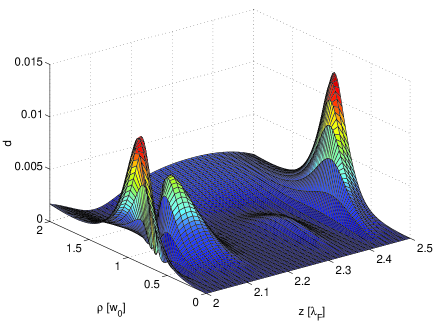
FIG. 3.: For parameters to be used later, $S_{0}/(2\pi)=50$MHz, and $\Delta_{p}/(2\pi)=-10$MHz, $N_{e}=0.01$ we plot here the ratio $d=D_{zx}^{2}/(D_{zz}D_{xx})$ as a function of position.

Thus, friction is appreciable only along the cavity axis, while diffusion has two main contributions: from spontaneous emission in all three directions, and a large diffusion along the cavity axis from fluctuations in the FORT and cavity QED forces.

IV Numerical results

The following results pertain to a Cs atom, with the ground state given by $|6S_{1/2};F=4;m_{F}=4\rangle$ and the excited state by $|6P_{3/2};F=5;m_{F}=5\rangle$, so that $\lambda_{0}=852.4$nm and $\Gamma/(2\pi)=5.2$MHz. The cavity parameters are $\kappa/(2\pi)=4$MHz and $g_{0}/(2\pi)=30$MHz, and $w_{0}=20\mu$, which are typical for the experiments discussed in [6]. Furthermore, the values for $S_{0}$ examined here are $S_{0}/(2\pi)=10,50$MHz. Both of these values are close to those explored in the actual experiment [6], and they contrast the behavior of atoms in shallow ($S_{0}<g_{0}$) and deep ($S_{0}>g_{0}$) wells. Typical values for $N_{e}$ range from $10^{-3}$ to 0.1.

A Dressed state structure

We first focus on the atomic motion along the cavity axis. The simplest way to get a feeling for the results for $\beta_{zz}$ and $D_{zz}$ as a function of the probe detuning $\Delta_{p}$ is to first consider the eigenenergies of the dressed atom-cavity states. When we neglect dissipation for the moment, and take the limit of no driving ($N_{e}=0$), we can easily find the energies of the lower dressed states $|\psi_{\pm}\rangle$ containing at most one excitation: the state containing no excitation is the ground state with an energy of $E_{0}=-\hbar S_{F}(\vec{r})$, while the energies of the two dressed states in the manifold of states containing a single excitation are

$$E_{\pm}=\hbar\omega_{a}\pm\hbar\sqrt{g(\vec{r})^{2}+S_{F}(\vec{r})^{2}},$$ (31)

if the atom and cavity are on resonance. The excited dressed states are given by

$$|\psi_{-}\rangle=\sin\theta|g,1\rangle+\cos\theta|e,0\rangle,$$ (32)

with

$$\sin\theta = \frac{g}{\sqrt{g^{2}+(\sqrt{g^{2}+S_{F}^{2}}-S_{F})^{2}}},$$ (33)

$$\cos\theta = \frac{S_{F}-\sqrt{g^{2}+S_{F}^{2}}}{\sqrt{g^{2}+(\sqrt{g^{2}+S_{F}^{2}}-S_{F})^{2}}}.$$ (34)

In Figures 4 (10MHz FORT) and 5 (50MHz FORT) we plot the transition frequencies (relative to $\omega_{a}$) from the ground state to these two excited states as functions of position, i.e.,

$$\Delta_{\pm}=S_{F}(\vec{r})\pm\sqrt{g(\vec{r})^{2}+S_{F}(\vec{r})^{2}}.$$ (35)

This expression along with the figures explicitly shows that the main features of the atom-cavity system are determined by the ratio $S_{0}/g_{0}$. It furthermore shows an important difference with the situation of trapping with a FORT in free space. The fact that the excited state shifts up while the ground state shifts down implies that ground and excited states are trapped in different positions in free space. In the presence of the quantized cavity field, however, both the lower excited dressed state and the ground state are now shifted down. This may improve trapping and cooling conditions, as detailed below.

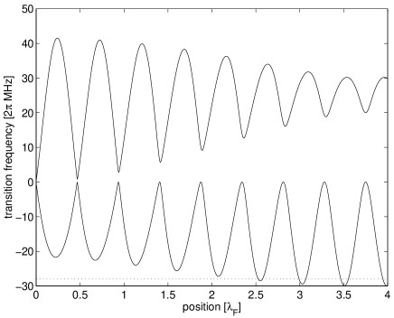
FIG. 4.: Transition frequencies $\Delta_{\pm}$ relative to the bare atomic frequency from the ground state to the lower two excited dressed states as functions of the position of the atom along the cavity axis (i.e. $\rho=0$) . Here $S_{0}/(2\pi)=10$MHz. Also indicated by the dotted line is the probe detuning used in Fig. 9, $\Delta_{p}/(2\pi)=-28$MHz.

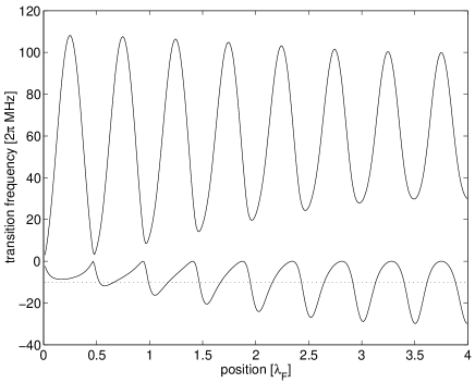
FIG. 5.: Same as previous figure but for $S_{0}/(2\pi)=50$MHz. Also indicated by the dotted line is the probe detuning used in Figure 10, $\Delta_{p}/(2\pi)=-10$MHz.

B Cooling mechanisms

We now take a closer look at cooling mechanisms. In the regime of weak driving, we will find that the friction coefficient $\beta_{zz}$ is positive (corresponding to cooling) when the probe field is tuned slightly (by an amount $~{}\sim\kappa,\Gamma/2$) below the transition to the relevant dressed state while for blue detuning the friction coefficient is negative, leading to exponential heating of the atom’s velocity. This can be understood by analogy with Doppler cooling: by tuning below resonance, the process of stimulated absorption followed by spontaneous emission leads to a loss of energy, while the maximum cooling rate is achieved by maximizing the product of excitation rate and detuning. Now looking back to Figs. 4 and 5 one sees that the variation of $\Delta_{+}$ with position is larger than that of $\Delta_{-}$, because both the ground state and the lower excited dressed state shift down, while the upper excited dressed state shifts upward. Generally speaking, for cooling purposes it is better to tune to the lower excited state so as to have smaller spatial variations in cooling rates. More importantly, the upper excited state energies decrease with increasing radial distance, whereas the lower excited state energy increases. Thus, for the upper state the probe detuning changes from red to blue, so that an atom cooled on axis will in fact be heated if it moves away radially. For the lower dressed state the probe detuning becomes more red, so that an atom that is optimally cooled on axis will still be cooled away from the axis, but at a lower rate.

The most popular explanation for intra-cavity cooling [10] exploits analogies with Sisyphus cooling [21], although another explanation for cavity-based cooling based on asymmetries in coherent scattering was recently put forward in [11]. Here we illustrate the Sisyphus picture for cooling inside optical wells within an optical resonator, using a very simple dressed-state picture, that makes use of only the lower dressed state and the ground state, relevant in the low-excitation limit. We choose one particular well, from $z=2.0\lambda_{F}$ to $z=2.5\lambda_{F}$, and one particular set of parameters given in the caption of Fig. 6. In that figure we plot the decay rate $\gamma_{-}$ of the lower dressed state and the excitation rate from ground to the dressed state, $\Omega_{-}$, as functions of position. In the weak driving limit the decay rate is given by

$$\gamma_{-} = \langle\psi_{-}|\kappa a^{+}a+\Gamma\sigma^{+}\sigma^{-}/2|\psi_{-}\rangle$$ (36)

$$= \sin^{2}\theta\kappa+\cos^{2}\theta\Gamma/2,$$ (37)

and the excitation rate by

$$\Omega_{-} = |\langle g,0|{\cal E}_{0}(a^{+}+a)|\psi_{-}\rangle|$$ (38)

$$= {\cal E}_{0}|\sin\theta|.$$ (39)

These two quantities, together with the detuning of the probe field from (dressed-state) resonance determine the steady-state population in the lower dressed state, according to

$$n_{-}=\frac{\Omega_{-}^{2}}{(\Delta_{-}-\Delta_{p})^{2}+\gamma_{-}^{2}}.$$ (40)

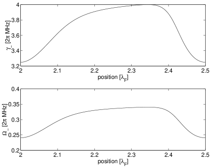
FIG. 6.: Decay rate and excitation rate of the lower dressed state as functions of position along the cavity axis ($\rho=0$). Here and in Figures 7 and 8, we chose the following parameters: $N_{e}=0.001$, $S_{0}/(2\pi)=50$MHz, $\Delta_{p}/(2\pi)=-10$MHz.

The population $n_{-}$ is plotted in Fig. 7, along with the transition frequency $\Delta_{-}$. These two quantities are sufficient to understand the Sisyphus cooling mechanism.

FIG. 7.: Transition frequency to and populations in the lower dressed state as functions of position along the cavity axis. Note that the equilibrium position of the atom is around $z=2.25\lambda_{F}$.

Since an atom in the ground state is moving in a conservative potential around the equilibrium position $z=2.25\lambda_{F}$, the following Sisyphus picture should be taken as to apply to the motion of the atom in addition to that conservative motion (see (41)). Suppose, for example, that the atom is at position $z=2.2\lambda_{F}$ and moving towards the right (cf. Fig. 7). The probability to be in the excited state now decreases (according to the lower part of Fig. 7), while the energy of the excited state relative to the ground state is increasing: in other words, an atom in the excited state is climbing uphill (again, in relation to the ground state), but will likely make the down transition to the ground state, thus leading to cooling at that particular position. Similarly, at $z=2.4\lambda_{F}$ an atom moving to the left is going uphill while having an increased chance of decaying to the ground state, again leading to cooling. This picture in fact shows that the cooling rate is expected to be proportional to the gradient of $n_{-}$ and the gradient of $\Delta_{-}$. More precisely, the force on the atom at position $z$ is approximately given by

$$F_{z} \approx \hbar\frac{dS_{F}}{dz}-\hbar n_{-}(z-v/\gamma_{-})\frac{d\Delta_{-}}{dz}$$ (41)

$$\approx \hbar\frac{dS_{F}}{dz}-\hbar n_{-}(z)\frac{d\Delta_{-}}{dz}+\frac{\hbar v}{\gamma_{-}}\frac{dn_{-}}{dz}\frac{d\Delta_{-}}{dz},$$ (42)

where the argument of $n_{-}$ indicates the lag between the atom reaching a position $z$ and reaching its steady state, with the lag time scale determined by the inverse decay rate from the dressed state. From the second line we see that the friction coefficient $\beta_{zz}$ is approximated by

$$R\equiv-\frac{\hbar}{m\gamma_{-}}\frac{dn_{-}}{dz}\frac{d\Delta_{-}}{dz}.$$ (43)

Indeed, Fig. 8 shows the similar behavior of $\beta_{zz}$ and $R$ as functions of position.

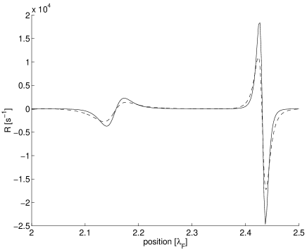
FIG. 8.: Cooling rate $\beta_{zz}$ (solid curve) and the product of gradients of dressed-state population and transition frequency $R$ (dashed curve) as functions of position along the cavity axis. The similarity between the two curves confirms the validity of the Sisyphus cooling picture.

C Friction, diffusion and equilibrium rms velocities

In Figures 9–10 we give examples of friction and diffusion coefficients for both the 10 and 50 MHz FORTs, as functions of the atomic position. They illustrate the point that in the low-excitation limit red (blue) detuning leads to cooling (heating) (cf. Figs. 4 and 5). They moreover clearly show how all wells are quantitatively different, with cooling rates and diffusion strengths differing by orders of magnitude over the various wells, and with $\beta_{zz}$ being negative in some wells, and always positive in others. This of course also implies that the temperatures reached by atoms in thermal equilibrium vary with position.

FIG. 9.: Friction and velocity diffusion coefficients $\beta_{zz}$ and $D_{zz}$ as functions of the atomic position (in units of $\lambda_{F}$) along the cavity axis. Here $N_{e}=0.001$, $S_{0}/(2\pi)=10$MHz, and $\Delta_{p}=-28\times 2\pi$MHz. Cf. Fig. 4.

For the case of the shallow FORT we consider weak driving ($N_{e}=0.001$), whereas for the deeper FORT the driving field is taken to be stronger by an order of magnitude. The stronger driving field increases cooling rates while the fact that deeper wells trap the atoms better means that correspondingly larger diffusion rates still can be tolerated.

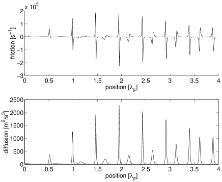
FIG. 10.: Same as previous Figure but for $N_{e}=0.01$, $S_{0}/(2\pi)=50$MHz, and $\Delta_{p}=-10\times 2\pi$MHz.

The stable equilibrium points $z^{e}_{n}$ are located around the maxima of $S_{F}$, i.e. around $z_{n}=(n-1/2)\lambda_{F}/2$ for integer $n$, because it is the FORT that gives the main contribution to the total force (even for the smallest value of $S_{0}=2\pi\times 10$MHz considered here). The cavity QED field gives only a small correction to the force and hence to the equilibrium position. In each equilibrium point, we can define a measure for the expected rms velocity of the atom along the $z$ axis in thermal equilibrium by considering averages over local wells

$$v_{{\rm rms}}^{z}=\sqrt{\frac{\bar{D}_{zz}}{\bar{\beta}_{zz}}}\,\,{\rm if}\,\bar{\beta}_{zz}>0,$$ (44)

in terms of the friction and diffusion coefficients. This averaging procedure gives a sensible measure for the rms velocity only if the atom indeed samples the whole well. This condition is fulfilled for the relatively shallow wells originating from $S_{0}=2\pi\times 10$MHz, and Fig. 11 uses this averaging procedure. For the 50MHz FORT, however, we averaged over only part of the well, namely a region of size $\lambda_{F}/10$ symmetrically around the equilibrium point. This choice is rather arbitrary, and thus Fig. 12 just gives an indication of what rms velocities to expect for atoms trapped in the corresponding wells, although the simulations in fact do confirm these values.

FIG. 11.: The values of $v_{{\rm rms}}^{z}$ in the eight equilibrium points as defined in (44) by averaging over the entire well. In all cases $S_{0}=2\pi\times 10$MHz. Triangles correspond to a detuning $\Delta_{p}/(2\pi)=-28$MHz, squares to $\Delta_{p}/(2\pi)=-23$MHz, and circles to $\Delta_{p}/(2\pi)=15$MHz . Note the points on the latter curve on the axis indicate that the friction coefficient is negative, so that there is in fact no cooling and $v_{{\rm rms}}^{z}$ is not defined. They do not indicate cooling to $v_{{\rm rms}}=0$.

FIG. 12.: As previous Figure, but for $S_{0}=2\pi\times 50$MHz and $N_{e}=0.01$, and where the average is taken over a region of size $\lambda_{F}/10$ around the equilibrium point. The probe detunings were $\Delta_{p}/(2\pi)=-10,-5,100$MHz for the squares, triangles, and circles, respectively. Note the points on the axis indicate that the friction coefficient is negative, so that there is in fact no cooling and $v_{{\rm rms}}^{z}$ is not defined. They do not indicate cooling to $v_{{\rm rms}}=0$.

We see here that depending on the probe detuning, the atom will be cooled to low temperatures either in all wells, or only in wells where $g$ is large in the equilibrium point, or only in wells where $g$ is small. This shows the flexibility that a FORT beam adds: one can predetermine to a certain degree in which well the atom will be trapped (and cooled) for longer times and in which it will not be.

Under the current conditions $\kappa>\Gamma/2$ the lowest temperatures achievable are determined by the Doppler velocity $v_{D}$. More precisely, the lower limit on rms velocities along the cavity axis is expected to be

$$v_{D}^{z}=\sqrt{0.7\frac{\hbar\Gamma}{2m}},$$ (45)

where the factor $0.7=(1+2/5)/2$ comes from the fact that in our case the diffusion due to spontaneous emission in the $z$ direction is 2/5th of the full 3-D value. We tested that for smaller $\kappa$ the rms velocities indeed do become even smaller, now determined by $\sqrt{\hbar\kappa/m}$, thus confirming predictions of [10].

Finally, we note that the quasiclassical approximation used throughout this paper is justified as neither the recoil limit is reached nor the resolved-sideband limit, i.e.

$$\hbar\Gamma/2 \gg (\hbar k)^{2}/m,$$ (46)

$$\hbar\Gamma/2 \gg h\nu_{{\rm osc}},$$ (47)

with $\nu_{{\rm osc}}$ the oscillation frequency of the atom in a well (see below), although in some cases the latter condition is only marginally fulfilled, namely when $\nu_{{\rm osc}}=600$kHz, which is only a factor 4 smaller than $\Gamma/(4\pi)$.

D Saturation behavior

We now briefly turn to the question of the nonlinear behavior of the atom-cavity system with increasing excitation. In the absence of saturation effects, both friction and diffusion coefficients would increase linearly with $N_{e}$. For the same parameters as Fig. 9, Figure 13 shows nonlinearities setting in around $N_{e}=0.01$. The friction coefficient even starts to decrease around $N_{e}=0.1$ as a result of the local values of $\beta_{zz}$ becoming negative where they were positive in the weak driving limit. The concomitant effect on the $v_{{\rm rms}}^{z}$ is shown as well.

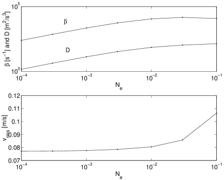
FIG. 13.: The average values of $D_{zz}$ and $\beta_{zz}$ as functions of the driving field strength $N_{e}$ in the well extending from $z=2\lambda_{F}$ to $z=2.5\lambda_{F}$, for the 10 MHz FORT, where $\Delta_{p}=-28\times 2\pi$MHz. In the lower part the corresponding values for the rms velocity $v_{{\rm rms}}^{z}$ are plotted as a function of $N_{e}$.

E Simulations

We also performed Monte-Carlo simulations of the 3-D motion in given wells by solving the Langevin equations (13) for position and velocity (see also [14]). The experimental procedure switches the FORT field on only when an atom has been detected and when it consequently has partly fallen through the cavity already [6]. We accordingly fix initial conditions as follows: We start the atom on the cavity axis, and we fix the downward velocity to be $v_{x}=10$ cm/s. Furthermore, we chose $v_{z}=0$ cm/s, and the initial position along the $z$ axis to be $\lambda_{F}/8$ away from the equilibrium point. The initial position and velocity were fixed so that all variations in trapping times and rms velocities are solely due to the random fluctuations of the forces acting on the atom, rather than from random initial conditions. Experimentally these two are mixed of course.

Since atoms with these initial conditions do not possess angular momentum around the $z$ axis, this in some sense represents a favorable case (although the atoms are not put in the bottom of the well). However, in the course of their evolution the atoms do acquire angular momentum so that this is in fact not a severe restriction. For more detail see below (Figure 22).

In Figure 14 we plot the results of simulations of 1000 trajectories for an atom in the shallow well of 10 MHz. We plot the average rms velocity along the cavity axis as a function of trapping time for each trajectory. Here we defined the “trapping time” as the time spent by the atom in one particular given well of size $\lambda_{F}/2$. The actual trapping time inside the cavity may be longer, obviously, as the atom may subsequently get trapped in different wells. For very short trapping times, $v_{rms}$ is determined by the initial condition, but for longer times lower temperatures corresponding to those calculated in Fig.11 are reached. Note however that the simulations were done in 3-D, and as such do not necessarily give the same temperatures as predicted for on-axis (1-D) motion in Figures 11 and 12. Nevertheless, the effect of the atoms’ radial motion is apparently not strong, and in fact atoms leave the well while still being trapped radially. This is partly due to the fact that all (especially heating) rates in the radial direction are smaller by a factor $kw_{0}\approx 150$ than those in the axial direction.

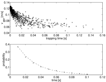
FIG. 14.: In the upper part of the plot each data point gives the trapping time and the average $v_{{\rm rms}}$ resulting from a single trajectory. Identical initial conditions were chosen for each trajectory: each atom started at $z=2.125\lambda_{F}$ with $v_{z}=0$ and $v_{x}=10$cm/s (downward). Other parameters were: $N_{e}=0.001$, $\Delta_{p}=-28\times 2\pi$MHz, $S_{0}=10\times 2\pi$MHz. The lower part gives a histogram of the probability $P(T)$ for an atom to be trapped longer than a time $T$. A fit of the tail of this distribution to an exponential $\propto\exp(-T/\tau)$ gives $\tau=(25\pm 2)$ ms

About half of the atoms is basically not trapped at all. The remaining atoms have a probability $P(T)$ to be trapped longer than a time $T$, with $P(T)$ decaying exponentially with $T$. The average trapping time for these parameters is found to be $\tau\approx$ 25ms, as shown in Fig. 14.

In Figures 15 and 16 we plot for the same 10MHz FORT an example of a single trajectory, after the atom has spent 4ms in the trap. The oscillation frequencies along the $z$ and the radial directions differ by two orders of magnitude (since $kw_{0}\approx 150$): in the $z$ direction the oscillation rate is $\sim$ 200kHz, in the radial direction $\sim$ 2.2kHz. The photon transmission follows both these oscillations so that in principle the atomic motion in both axial and radial direction is detectable. Experimentally, though, the oscillations along the cavity axis may be too fast to be accessible. In particular, the average rate at which photons leaking out through one end of the cavity are detected is at most (the efficiency is less than 100%) equal to the cavity decay rate multiplied by the average number of photons inside the cavity. For the parameters of Fig. 15 this amounts to a rate $\sim 0.01\times\kappa\approx 2.5\times 10^{5}$/sec, which corresponds to just about one photon per oscillation period.

The figures show that when the atom is in a position where it is not coupled to the cavity ($g=0$), the number of photons in the cavity drops to $N_{e}=0.001$. Similarly, when the atom moves away radially, the transmission drops.

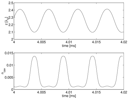
FIG. 15.: Snapshot of a single trajectory, with parameters as in Figure 14. The upper plot gives the $z$ coordinate of the atom as a function of time, the lower plot gives the transmission (in fact the number of photons $\langle a^{+}a\rangle$ inside the cavity) in that same time interval. Note the time scales here differ by two orders of magnitude from those of Figure 16.

FIG. 16.: For the same trajectory as the previous figure, the upper plot gives the radial distance to the cavity axis, $\rho$ in units of $w_{0}$ as a function of time, the lower plot gives again the number of photons inside the cavity during that same time interval. The atom has a nonzero angular momentum along $z$ and does not cross the $z$ axis.

To make a direct comparison with the trapping times achieved in the experiment [6], we now turn to the case of a 50 MHz FORT. We plot rms velocities vs trapping times for 300 trajectories for an atom trapped in the well ranging from $z=2\lambda_{F}$ to $z=2.5\lambda_{F}$.

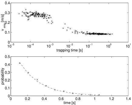
FIG. 17.: As Fig. 14 but for $N_{e}=0.01$, $\Delta_{p}=-10\times 2\pi$MHz, $S_{0}=50\times 2\pi$MHz. The mean trapping time is $\tau=250\pm 20$ms.

For the parameters of Fig. 17 the atom is either trapped for long times ($>10$ms) or only for a short time ($<1$ms), both with about $50\%$ probability. In the latter case the rms velocity is determined just by the (arbitrarily chosen) initial condition and is around 30cm/s, but for longer trapping times the effects of cooling are visible. Thermal equilibrium is reached with $v_{rms}\sim 8$cm/s, thus confirming the results of Fig. 12. The distribution of trapping times again follows an exponential law, and the average trapping time, as determined from the tail of the distribution, is $\tau\approx 250$ms, which is ten times longer than for the (fluctuating) 50MHz FORT used in [6]. This shows the great potential of holding single atoms in the cavity for extended periods of time if the intensity fluctuations of the FORT beam can be minimized. Experimental efforts along this path are currently underway.

Also for this case we plot snapshots for a single trajectory, taken after the atom has spent 25ms in the trap. Compared to the 10MHz FORT, the oscillations of the atom along the cavity axis and in the radial direction become faster by about a factor of 3. The axial oscillation frequency is about 600kHz, while along the radial direction the oscillations occur at a rate 6.2kHz, i.e., again slower by two orders of magnitude. In this case, the photon transmission still follows directly the axial oscillations but no longer follows the radial excursions of the atom, as now the fluctuations in the magnitude of $g$ at the atom’s position along the cavity axis are in fact larger than those due to the radial excursions of the atom. This is partly due to the fact that in the simulations here the driving field is stronger than for the 10MHz example above so that fluctuations in the atomic motion occur at a shorter time scale, and partly simply because the radial excursions are small. Fig. 19(c) shows that it is primarily the axial fluctuations that determine the variations in the numbers of photons inside the cavity.

Generally speaking, the axial excursions determine (local) minimum and maximum transmission levels (as in Fig. 15). When these minima and/or maxima depend on the radial position, then the radial motion could in principle be visible in the cavity transmission level. This depends in turn on whether the axial fluctuations on the time scale of the transverse motion are sufficiently small so as not to hide the radial dependence. There seems to be no simple general rule how this interplay between radial and axial motions depends on detunings, driving strength, and the particular well.

FIG. 18.: Snapshot of a single trajectory, with parameters as in Figure 17. The upper plot gives the $z$ coordinate of the atom as a function of time (with the atom released with standard initial conditions at $t=0$). The lower plot gives the transmission (in fact the number of photons inside the cavity) in that same time interval. Note the time scales here differ by two orders of magnitude from those of Figure 19.

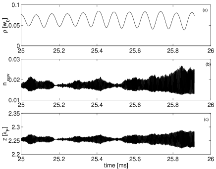
FIG. 19.: For the same trajectory as the previous figure, (a) the radial distance to the cavity axis, $\rho$ in units of $w_{0}$ as a function of time, (b) the number of photons inside the cavity during that same time interval, and (c) the position along the cavity axis in units of $\lambda_{F}$.

In contrast, in a different well, the one ranging from $z=0.0$ to $z=0.5\lambda_{F}$, the photon number in the cavity does follow the radial motion, as the radial excursions become larger. Perhaps more importantly, the average transmission level is higher by more than a factor 2 compared to the previous case, as a result of $g$ being larger in this well (cf. Fig. 2). This shows how, in principle, different wells may be experimentally distinguished via the transmission of the probe field through the cavity.

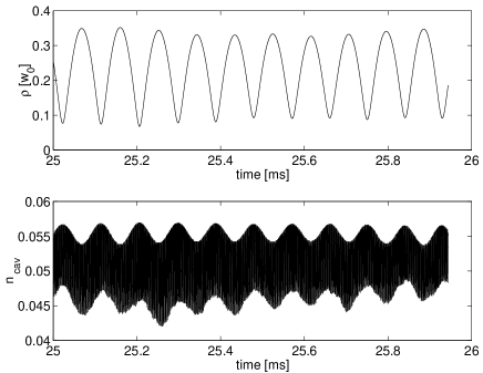
FIG. 20.: For an atom in the well ranging from $z=0$ to $z=\lambda_{F}/2$, for $N_{e}=0.01$, $\Delta_{p}=-10\times 2\pi$MHz, and $S_{0}=50\times 2\pi$MHz, the upper plot gives the radial distance to the cavity axis, $\rho$ in units of $w_{0}$ as a function of time, the lower plot gives the number of photons inside the cavity during that same time interval.

We also simulated the motion of an atom trapped under more adverse conditions, namely for an atom in the well $[z=\lambda_{F}\rightarrow 1.5\lambda_{F}]$ at a probe detuning $\Delta_{p}/(2\pi)=-5$MHz. According to Fig. 12, the atom is not cooled on axis under these conditions (i.e. the average friction coefficient around the equilibrium point on the $z$ axis is negative). This is confirmed by Fig. 21: the mean trapping time for an atom starting at $z=1.125\lambda_{F}$ is now very short, about 1.6ms, while the average rms velocity is $v_{{\rm rms}}^{z}\approx 28$ cm/s, as determined essentially by the initial condition.

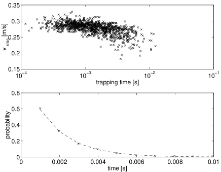
FIG. 21.: As Fig. 14 but for $N_{e}=0.01$, $\Delta_{p}=-5\times 2\pi$MHz, $S_{0}=50\times 2\pi$MHz. The initial position of the atom is $z=1.125\lambda_{F}$. The mean trapping time is $\tau=1.6\pm 0.1$ms.

Finally, we consider the influence of different initial conditions on trapping and cooling. All the results so far were obtained by considering atoms that initially are moving on axis. Thus, they have no angular momentum along the $z$ axis, nor any radial potential energy. Figure 22 shows a plot of rms velocities vs. trapping times for atoms trapped under the same conditions as for Fig. 17) (i.e., in the well from $z=2\lambda$ to $z=2.5\lambda$, for $\Delta_{p}=-10\times 2\pi$MHz, $N_{e}=0.01$, and $S_{0}=50\times 2\pi$MHz), but with different (nonzero) values for the initial angular momentum.

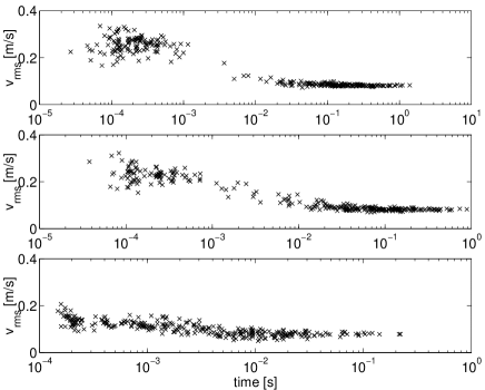
FIG. 22.: Rms velocities vs. trapping times for atoms trapped under the same conditions as for Fig. 17 but with different initial radial conditions for $y$. In particular, for plot (a) the initial conditions on $y$ is $y=0.2w_{0}$. for (b) $y=0.5w_{0}$ and for (c) $y=w_{0}$. Since $v_{x}=-10$cm/s, the atoms have different angualr momenta along $z$ in these cases, and different initial potential energies.

Obviously, the more initial potential energy the atom has, the less likely it is to be trapped. In fact, the angular momentum does not play any role here, as confirmed by similar calculations with initial conditions chosen such that the atoms have no initial angular momentum but have the same potential energy. The results are the same in that case. For atoms starting at $y=0.2w_{0}$ the trapping times and rms velocities are basically not affected, and the trapping time is still around 250ms. But for atoms starting at $y=0.5w_{0}$ the effect of their increased potential energy leads to clearly shorter trapping times (by roughly a factor of 2), and for atoms starting at $y=w_{0}$ this effect is even more pronounced with a decrease in trapping time of about a factor of 10.

F A different trapping structure

We now consider a different case where the atomic excited state is assumed to be shifted down by the FORT field, just as the ground state is (see, for instance [12]). This can be achieved by using a FORT that is (red) detuned in such a way that the excited atomic state is relatively closer to resonance with a higher-lying excited state than with the ground state. This situation at first sight looks even more appealing for trapping purposes, as now both excited and ground state will be trapped in the same positions. Moreover, fluctuations in the force due to the FORT are dimished.

We consider only the 50MHz FORT here, and compare this case to the previous 50MHz FORT case, and in particular we refer the reader back to Figs. 5, 10, and 17. For ease of comparison we keep $\lambda_{F}$ the same, and assume for simplicity that the excited state is shifted down by an amount $S_{F}$, so that the shifts of the ground and excited state are in fact identical.

The fact that ground and excited state see the same potential, implies that the transition frequencies to the dressed states are simply periodic in space with period $\lambda_{0}$, as shown in Fig. 23, rather than aperiodic as in Fig. 5.

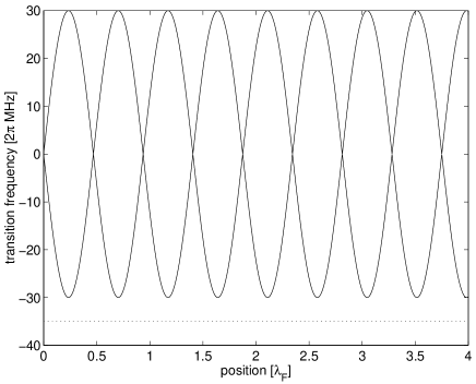
FIG. 23.: Transition frequencies $\Delta_{\pm}$ for the case where the atomic excited state is assumed to be shifted down by the FORT field by the same amount $S_{F}$ as is the ground state, for the 50MHz FORT. A detuning of $-35$MHz is indicated by the dotted line.

Similarly, the fluctuations in the force due to the FORT now vanish, as both ground and excited state undergo the same shift, so that the diffusion coefficient is periodic with period $\lambda_{0}$. Also the friction force arises only from the cavity QED part and is periodic. Yet, the different wells are not equivalent. The forces are, just as before, driven by both cavity QED field and the FORT, and the value of $g$ at the antinode of the FORT still varies over the different wells. This is illustrated in Fig. 24 where the rms velocities in the 8 different wells are shown, along with friction and diffusion coefficients. Since in this example the probe field is detuned below the lower dressed state, one has cooling everywhere in space.

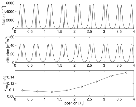
FIG. 24.: Friction and diffusion coefficients, and the resulting rms velocity as functions of position along the cavity axis for the trapping structure of Section IV F. Here $\Delta_{p}/(2\pi)=-35$MHz, and $N_{e}=0.01$.

The simulations show that the mean trapping time is smaller, although the rms velocities are just as small as before. The reason is the less favorable cooling condition away from the cavity axis. In particular, for the parameters used here the expected rms velocity $v_{{\rm rms}}^{z}$ steadily increases to 90cm/s at a radial distance $\rho=2w_{0}$, while for the simulations of Figs. 17, $v_{{\rm rms}}^{z}$ is increasing only slowly to 12cm/s. This large difference can be understood by noting the difference in dressed state structures between the two cases. For the case of Fig. 5, the transition frequency to the lower dressed state around the equilibrium position $z\approx 2.25\lambda_{F}$ does not change much with increasing radial distance, so that the probe field in that trapping region is always detuned below resonance by an amount that stays more or less constant. For the dressed state structure of Fig. 23, however, the probe detuning increases from $\geq 5$MHz to $\geq 35$MHz below resonance, thus leading to much worse cooling conditions. In other words, the presence of opposite level shifts due to the FORT makes the spatial variation of the transition frequency to the lower dressed state smaller: compare $\Delta_{-}=S_{F}-\sqrt{S_{F}^{2}+g^{2}}$ to $\Delta_{-}=-g$, especially when $g\ll S_{F}$.

The alternative trapping potential is, therefore, not necessarily more favorable for trapping purposes. On the other hand, all atoms are captured now and are trapped for at least 10ms. This can be understood from the simple fact that here the friction coefficient is positive in the entire well.

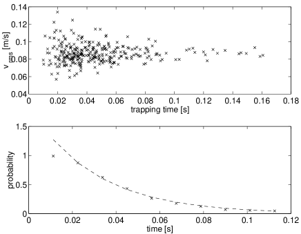
FIG. 25.: As Figure 14, but for the different trapping structure of Section IV F. The initial position was $z=0.125\lambda_{F}$, and further parameters were $N_{e}=0.01$, $\Delta_{p}=-35\times 2\pi$MHz, $S_{0}=50\times 2\pi$MHz. The mean trapping time is $\tau=28\pm 2$ms.

V Summary

We analyzed cooling limits and trapping mechanisms for atoms trapped in optical traps inside optical cavities. The main distinguishing feature from previous discussions on cooling of atoms inside cavities is the presence of the external trapping potential with a different spatial periodicity as compared to the cavity QED field. This not only provides better cooling and trapping conditions but the different spatial period makes the various potential wells qualitatively different. Atoms can be trapped in regions of space where the coupling to the cavity QED field is maximum, minimum or somewhere in between. Depending on the laser detuning, cooling may take place only in wells where the atom is minimally coupled to the cavity QED field, or where it is maximally coupled. This allows one in principle to distinguish to a certain degree the different atomic positions along the cavity axis, namely, by comparing

• the average transmission level

• the fluctuations of the cavity transmission

• the total trapping time

which reflect, respectively, the average atom-cavity coupling, the temperature of the atom and under certain conditions the radial motion, and the overall cooling and trapping conditions. This is an important additional tool useful for eventual control of coherent evolution of the atomic center-of-mass degrees of freedom, as relevant to performing quantum logic operations.

REFERENCES

- [1] C.J. Hood, T.W. Lynn, A.C. Doherty, A.S. Parkins, and H.J. Kimble, Science 287, 1447 (2000).
- [2] P.W.H. Pinkse, T. Fischer, P. Maunz, and G. Rempe, Nature 404, 365 (2000).
- [3] A.C. Doherty, C.J. Hood, T.W. Lynn, and H.J. Kimble, in preparation.
- [4] J.I. Cirac, P. Zoller, H.J. Kimble and H. Mabuchi, Phys. Rev. Lett. 78, 3221 (1997).
- [5] S.J. van Enk, J.I. Cirac and P. Zoller, Phys. Rev. Lett. 78, 4293 (1997); Science 279, 205 (1998).
- [6] J. Ye, D.W. Vernooy and, H.J. Kimble, Phys. Rev. Lett. 83, 4987 (1999).
- [7] C.W. Gardiner, J. Ye, H.C. Nägerl, and H.J. Kimble, Phys. Rev. A 61, 045801 (2000).
- [8] H.C. Nägerl, D. Stamper-Kurn, J. Ye, and H.J. Kimble, to be published.
- [9] T.W. Mossberg, M. Lewenstein and D.J. Gauthier, Phys. Rev. Lett. 67, 1723 (1991).
- [10] P. Horak, G. Hechenblaikner, K.M. Gheri, H. Stecher, and H. Ritsch, Phys. Rev. Lett. 79, 4974 (1997). G. Hechenblaikner, M. Gangl, P. Horak, and H. Ritsch, Phys. Rev. A 58, 3030 (1998).
- [11] V. Vuletic and S. Chu, Phys. Rev. Lett. 84, 3787 (2000) and references therein.
- [12] H.J. Kimble, C.J. Hood, T.W. Lynn, H. Mabuchi, D.W. Vernooy, and J. Ye, Laser Spectroscopy XIV, Eds. R. Blatt et al., World Scientific (Singapore, 1999).
- [13] For a review of older work on quantized atomic motion in the context of cavity QED, see P. Meystre, Progress in Optics XXX, 263 (1992), Editor E. Wolf, (North-Holland, Amsterdam). For a more recent review, see H. Walther, Phys. Scripta T76, 138 (1998); see also D.W. Vernooy and H.J. Kimble, Phys. Rev. A 56, 4287 (1997) and references therein, in particular [3]–[18].
- [14] A.C. Doherty, A.S. Parkins, S.M. Tan, and D.F. Walls, Phys. Rev. A 56,833 (1997); ibid. 57, 4804 (1998).
- [15] R. Taieb, R. Dum, J.I. Cirac, P. Marte, and P. Zoller, Phys. Rev. A 49, 4876 (1994).
- [16] S. Marksteiner, K. Ellinger, and P. Zoller, Phys. Rev. A 53, 3409 (1996).
- [17] J. Dalibard and C. Cohen-Tannoudji, J. Phys. B 18, 1661 (1985).
- [18] C.W. Gardiner, Handbook of Stochastic Methods, 2nd Edition, Springer, Berlin (1997)
- [19] S.M. Tan, J. Opt. B 1, 424 (1999).
- [20] G.S. Agarwal and K. Mølmer, Phys. Rev. A 47, 5158 (1993).
- [21] J. Dalibard and C. Cohen-Tannoudji, J. Opt. Soc. Am. B 2, 1707 (1985).