On Quantum Detection and the Square-Root Measurement

Abstract

In this paper we consider the problem of constructing measurements optimized to distinguish between a collection of possibly non-orthogonal quantum states. We consider a collection of pure states and seek a positive operator-valued measure (POVM) consisting of rank-one operators with measurement vectors closest in squared norm to the given states. We compare our results to previous measurements suggested by Peres and Wootters [11] and Hausladen et al. [10], where we refer to the latter as the square-root measurement (SRM). We obtain a new characterization of the SRM, and prove that it is optimal in a least-squares sense. In addition, we show that for a geometrically uniform state set the SRM minimizes the probability of a detection error. This generalizes a similar result of Ban et al. [7].

1 Introduction

Suppose that a transmitter, Alice, wants to convey classical information to a receiver, Bob, using a quantum-mechanical channel. Alice represents messages by preparing the quantum channel in a pure quantum state drawn from a collection of known states. Bob detects the information by subjecting the channel to a measurement in order to determine the state prepared. If the quantum states are mutually orthogonal, then Bob can perform an optimal orthogonal (von Neumann) measurement that will determine the state correctly with probability one [1]. The optimal measurement consists of projections onto the given states. However, if the given states are not orthogonal, then no measurement will allow Bob to distinguish perfectly between them. Bob’s problem is therefore to construct a measurement optimized to distinguish between non-orthogonal pure quantum states.

We may formulate this problem as a quantum detection problem, and seek a measurement that minimizes the probability of a detection error, or more generally, minimizes the Bayes cost. Necessary and sufficient conditions for an optimum measurement minimizing the Bayes cost have been derived [2, 3, 4]. However, except in some particular cases [4, 5, 6, 7], obtaining a closed-form analytical expression for the optimal measurement directly from these conditions is a difficult and unsolved problem. Thus in practice, iterative procedures minimizing the Bayes cost [8] or ad-hoc suboptimal measurements are used.

In this paper we take an alternative approach of choosing a different optimality criterion, namely a squared-error criterion, and seeking a measurement that minimizes this criterion. It turns out that the optimal measurement for this criterion is the “square-root measurement” (SRM), which has previously been proposed as a “pretty good” ad-hoc measurement [9, 10].

This work was originally motivated by the problems studied by Peres and Wootters in [11] and by Hausladen et al. in [10]. Peres and Wootters [11] consider a source that emits three two-qubit states with equal probability. In order to distinguish between these states, they propose an orthogonal measurement consisting of projections onto measurement vectors “close” to the given states. Their choice of measurement results in a high probability of correctly determining the state emitted by the source, and a large mutual information between the state and the measurement outcome. However, they do not explain how they construct their measurement, and do not prove that it is optimal in any sense. Moreover, the measurement they propose is specific for the problem that they pose; they do not describe a general procedure for constructing an orthogonal measurement with measurement vectors close to given states. They also remark that improved probabilities might be obtained by considering a general positive operator-valued measure (POVM) [12] consisting of positive Hermitian operators $\Pi_{i}$ satisfying $\sum_{i}\Pi_{i}=I$, where the operators $\Pi_{i}$ are not required to be orthogonal projection operators as in an orthogonal measurement.

Hausladen et al. [10] consider the general problem of distinguishing between an arbitrary set of pure states, where the number of states is no larger than the dimension of the space ${\mathcal{U}}$ they span. They describe a procedure for constructing a general “decoding observable”, corresponding to a POVM consisting of rank-one operators that distinguishes between the states “pretty well”; this measurement has subsequently been called the square-root measurement (SRM) (see e.g., [13, 14, 15]). However, they make no assertion of (non-asymptotic) optimality. Although they mention the problem studied by Peres and Wootters in [11], they make no connection between their measurement and the Peres-Wootters measurement.

The SRM [7, 9, 10, 13, 14, 15] has many desirable properties. Its construction is relatively simple; it can be determined directly from the given collection of states; it minimizes the probability of a detection error when the states exhibit certain symmetries [7]; it is “pretty good” when the states to be distinguished are equally likely and almost orthogonal [9]; and it is asymptotically optimal [10]. Because of these properties, the SRM has been employed as a detection measurement in many applications (see e.g., [13, 14, 15]). However, apart from some particular cases mentioned above [7], no assertion of (non-asymptotic) optimality is known for the SRM.

In this paper we systematically construct detection measurements optimized to distinguish between a collection of quantum states. Motivated by the example studied by Peres and Wootters [11], we consider pure-state ensembles and seek a POVM consisting of rank-one positive operators with measurement vectors that minimize the sum of the squared norms of the error vectors, where the $i$th error vector is defined as the difference between the $i$th state vector and the $i$th measurement vector. We refer to the optimizing measurement as the least-squares measurement (LSM). We then generalize this approach to allow for unequal weighting of the squared norms of the error vectors. This weighted criterion may be of interest when the given states have unequal prior probabilities. We refer to the resulting measurement as the weighted least-squares measurement (WLSM). We show that the SRM coincides with the LSM when the prior probabilities are equal, and with the WLSM otherwise (if the weights are proportional to the square roots of the prior probabilities).

We then consider the case in which the collection of states has a strong symmetry property called geometric uniformity [16]. We show that for such a state set the SRM minimizes the probability of a detection error. This generalizes a similar result of Ban et al. [7].

The organization of this paper is as follows. In Section 2 we formulate our problem and present our main results. In Section 3 we construct a measurement consisting of rank-one operators with measurement vectors closest to a given collection of states in the least-squares sense. In Section 4 we construct the optimal orthogonal LSM. Section 5 generalizes these results to allow for weighting of the squared norms of the error vectors. In Section 7 we discuss the relationships between our results and the previous results of Peres and Wootters [11] and Hausladen et al. [10]. We obtain a new characterization of the SRM, and summarize the properties of the SRM that follow from this characterization. In Section 8 we discuss connections between the SRM and the measurement minimizing the probability of a detection error (MPEM). We show that for a geometrically uniform state set the SRM is equivalent to the MPEM. We will consistently use [10] as our principal reference on the SRM.

2 Problem Statement and Main Results

In this section, we formulate our problem and describe our main results.

2.1 Problem Formulation

Assume that Alice conveys classical information to Bob by preparing a quantum channel in a pure quantum state drawn from a collection of given states $\{{|\phi_{i}\rangle}\}$. Bob’s problem is to construct a measurement that will correctly determine the state of the channel with high probability.

Therefore, let $\{{|\phi_{i}\rangle}\}$ be a collection of $m\leq n$ normalized vectors ${|\phi_{i}\rangle}\,$in an $n$-dimensional complex Hilbert space ${\mathcal{H}}$. In general these vectors are non-orthogonal and span an $r$-dimensional subspace ${\mathcal{U}}\subseteq{\mathcal{H}}$. The vectors are linearly independent if $r=m$.

For our measurement, we restrict our attention to POVMs consisting of $m$ rank-one operators of the form $\Pi_{i}={|\mu_{i}\rangle}{\langle\mu_{i}|}$ with measurement vectors ${|\mu_{i}\rangle}\in{\mathcal{U}}$. We do not require the vectors ${|\mu_{i}\rangle}\,$to be orthogonal or normalized. However, to constitute a POVM the measurement vectors must satisfy

$$\sum_{i=1}^{m}\Pi_{i}=\sum_{i=1}^{m}{|\mu_{i}\rangle}{\langle\mu_{i}|}=P_{{\mathcal{U}}},$$ (1)

where $P_{\mathcal{U}}$ is the projection operator onto ${\mathcal{U}}$; i.e., the operators $\Pi_{i}$ must be a resolution of the identity on ${\mathcal{U}}$.

We seek the measurement vectors ${|\mu_{i}\rangle}\,$such that one of the following quantities is minimized:

1. Squared error $E=\sum_{i=1}^{m}{\langle e_{i}|e_{i}\rangle}$, where ${|e_{i}\rangle}={|\phi_{i}\rangle}-{|\mu_{i}\rangle}$;

2. Weighted squared error $E_{w}=\sum_{i=1}^{m}w_{i}{\langle e_{i}|e_{i}\rangle}$ for a given set of positive weights $w_{i}$.

2.2 Main Results

If the states ${|\phi_{i}\rangle}\,$are linearly independent (i.e., if $r=m$), then the optimal solutions to problems (1) and (2) are of the same general form. We express this optimal solution in different ways. In particular, we find that the optimal solution is an orthogonal measurement and not a general POVM.

If $r<m$, then the solution to problem (1) still has the same general form. We show how it can be realized as an orthogonal measurement in an $m$-dimensional space. This orthogonal measurement is just a realization of the optimal POVM in a larger space than ${\mathcal{U}}$, along the lines suggested by Neumark’s theorem [12], and it furnishes a physical interpretation of the optimal POVM.

We define a geometrically uniform (GU) state set as a collection of vectors ${\mathcal{S}}=\{{|\phi_{i}\rangle}=U_{i}{|\phi\rangle},U_{i}\in{\mathcal{G}}\}$, where ${\mathcal{G}}$ is a finite abelian (commutative) group of $m$ unitary matrices $U_{i}$, and ${|\phi\rangle}$ is an arbitrary state. We show that for such a state set the SRM minimizes the probability of a detection error.

Using these results, we can make the following remarks about [11] and the SRM [10]:

1. The Peres-Wootters measurement is optimal in the least-squares sense and is equal to the SRM (strangely, this was not noticed in [10]); it also minimizes the probability of a detection error.

2. The SRM proposed by Hausladen et al. [10] minimizes the squared error. It may always be chosen as an orthogonal measurement equivalent to the optimal measurement in the linearly independent case. Further properties of the SRM are summarized in Theorem 3 (Section 7).

3 Least-Squares Measurement

Our objective is to construct a POVM with measurement vectors ${|\mu_{i}\rangle}$, optimized to distinguish between a collection of $m$ pure states ${|\phi_{i}\rangle}\,$that span a space ${\mathcal{U}}\subseteq{\mathcal{H}}$. A reasonable approach is to find a set of vectors ${|\mu_{i}\rangle}\in{\mathcal{U}}$ that are “closest” to the states ${|\phi_{i}\rangle}\,$in the least-squares sense. Thus our measurement consists of $m$ rank-one positive operators of the form $\Pi_{i}={|\mu_{i}\rangle}{\langle\mu_{i}|},1\leq i\leq m$. The measurement vectors ${|\mu_{i}\rangle}\,$are chosen to minimize the squared error $E$, defined by

$$E=\sum_{i=1}^{m}{\langle e_{i}|e_{i}\rangle},$$ (2)

where ${|e_{i}\rangle}$ denotes the $i$th error vector

$${|e_{i}\rangle}={|\phi_{i}\rangle}-{|\mu_{i}\rangle},$$ (3)

subject to the constraint (1); i.e., the operators $\Pi_{i}$ must be a resolution of the identity on ${\mathcal{U}}$.

If the vectors ${|\phi_{i}\rangle}\,$are mutually orthonormal, then the solution to (2) satisfying the constraint (1) is simply ${|\phi_{i}\rangle}={|\mu_{i}\rangle},\,\,1\leq i\leq m$, which yields $E=0$.

To derive the solution in the general case where the vectors ${|\phi_{i}\rangle}\,$are not orthonormal, denote by $M$ and $\Phi$ the $n\times m$ matrices whose columns are the vectors ${|\mu_{i}\rangle}\,$and ${|\phi_{i}\rangle}$, respectively. The squared error $E$ of (2)-(3) may then be expressed in terms of these matrices as

$$E=\mbox{Tr}\left((\Phi-M)^{*}(\Phi-M)\right)=\mbox{Tr}\left((\Phi-M)(\Phi-M)^{*}\right),$$ (4)

where $\mbox{Tr}(\cdot)$ and $(\cdot)^{*}$ denote the trace and the Hermitian conjugate respectively, and the second equality follows from the identity $\mbox{Tr}(AB)=\mbox{Tr}(BA)$ for all matrices $A,B$. The constraint (1) may then be restated as

$$MM^{*}=P_{{\mathcal{U}}}.$$ (5)

3.1 The Singular Value Decomposition

The least-squares problem of (4) seeks a measurement matrix $M$ that is “close” to the matrix $\Phi$. If the two matrices are close, then we expect that the underlying linear transformations they represent will share similar properties. We therefore begin by decomposing the matrix $\Phi$ into elementary matrices that reveal these properties via the singular value decomposition (SVD) [17].

The SVD is known in quantum mechanics, but possibly not very well known. It has sometimes been presented as a corollary of the polar decomposition (e.g., in Appendix A of [18]). We present here a brief derivation based on the properties of eigendecompositions, since the SVD can be interpreted as a sort of “square root” of an eigendecomposition.

Let $\Phi$ be an arbitrary $n\times m$ complex matrix of rank $r$. Theorem 1 below asserts that $\Phi$ has a SVD of the form $\Phi=U\Sigma V^{*}$, with $U$ and $V$ unitary matrices and $\Sigma$ diagonal. The elements of the SVD may be found from the eigenvalues and eigenvectors of the $m\times m$ non-negative definite Hermitian matrix $S=\Phi^{*}\Phi$ and the $n\times n$ non-negative definite Hermitian matrix $T=\Phi\Phi^{*}$. Notice that $S$ is the Gram matrix of inner products ${\langle\phi_{i}|\phi_{j}\rangle}$, which completely determines the relative geometry of the vectors $\{{|\phi_{i}\rangle}\}$. It is elementary that both $S$ and $T$ have the same rank $r$ as $\Phi$, and that their nonzero eigenvalues are the same set of $r$ positive numbers $\{\sigma_{i}^{2},1\leq i\leq r\}$.

Theorem 1 (Singular Value Decomposition (SVD))

Let $\{{|\phi_{i}\rangle}\}$ be a set of $m$ vectors in an $n$-dimensional complex Hilbert space ${\mathcal{H}}$, let ${\mathcal{U}}\subseteq{\mathcal{H}}$ be the subspace spanned by these vectors, and let $r=\dim~{}{\mathcal{U}}$. Let $\Phi$ be the rank-$r$ $n\times m$ matrix whose columns are the vectors $\{{|\phi_{i}\rangle}\}$. Then

$$\Phi=U\Sigma V^{*}=\sum_{i=1}^{r}\sigma_{i}{|u_{i}\rangle}{\langle v_{i}|},$$

where

1. $\Phi^{*}\Phi=V(\Sigma^{*}\Sigma)V^{*}=\sum_{i=1}^{r}\sigma_{i}^{2}{|v_{i}\rangle}{\langle v_{i}|}$ is an eigendecomposition of the rank-$r$ $m\times m$ matrix $S=\Phi^{*}\Phi$, in which

   1. the $r$ positive real numbers $\{\sigma_{i}^{2},1\leq i\leq r\}$ are the nonzero eigenvalues of $S$, and $\sigma_{i}$ is the positive square root of $\sigma_{i}^{2}$;

   2. the $r$ vectors $\{{|v_{i}\rangle}\in\,\,{\mathbb{C}}^{m},1\leq i\leq r\}$ are the corresponding eigenvectors in the $m$-dimensional complex Hilbert space ${\mathbb{C}}^{m}$, normalized so that ${\langle v_{i}|v_{i}\rangle}=1$;

   3. $\Sigma$ is a diagonal $n\times m$ matrix whose first $r$ diagonal elements are $\sigma_{i}$, and whose remaining $m-r$ diagonal elements are $0$, so $\Sigma^{*}\Sigma$ is a diagonal $m\times m$ matrix with diagonal elements $\sigma_{i}^{2}$ for $1\leq i\leq r$ and $0$ otherwise;

   4. $V$ is an $m\times m$ unitary matrix whose first $r$ columns are the eigenvectors ${|v_{i}\rangle}$, which span a subspace ${\mathcal{V}}\subseteq{\mathbb{C}}^{m}$, and whose remaining $m-r$ columns ${|v_{i}\rangle}$ span the orthogonal complement ${\mathcal{V}}^{\perp}\subseteq{\mathbb{C}}^{m}$;

   and

2. $\Phi\Phi^{*}=U(\Sigma\Sigma^{*})U^{*}=\sum_{i=1}^{r}\sigma_{i}^{2}{|u_{i}\rangle}{\langle u_{i}|}$ is an eigendecomposition of the rank-$r$ $n\times n$ matrix $T=\Phi\Phi^{*}$, in which

   1. the $r$ positive real numbers $\{\sigma_{i}^{2},1\leq i\leq r\}$ are as before, but are now identified as the nonzero eigenvalues of $T$;

   2. the $r$ vectors $\{{|u_{i}\rangle}\in\,\,$${\mathcal{H}}$$,1\leq i\leq r\}$ are the corresponding eigenvectors, normalized so that ${\langle u_{i}|u_{i}\rangle}=1$;

   3. $\Sigma$ is as before, so $\Sigma\Sigma^{*}$ is a diagonal $n\times n$ matrix with diagonal elements $\sigma_{i}^{2}$ for $1\leq i\leq r$ and $0$ otherwise;

   4. $U$ is an $n\times n$ unitary matrix whose first $r$ columns are the eigenvectors ${|u_{i}\rangle}$, which span the subspace ${\mathcal{U}}\subseteq{\mathcal{H}}$, and whose remaining $n-r$ columns ${|u_{i}\rangle}$ span the orthogonal complement ${\mathcal{U}}^{\perp}\subseteq{\mathcal{H}}$.

Since $U$ is unitary, we have not only $U^{*}U=I_{\mathcal{H}}$, which implies that the vectors ${|u_{k}\rangle}\in{\mathcal{H}}$ are orthonormal, ${\langle u_{k}|u_{j}\rangle}=\delta_{kj}$, but also that $UU^{*}=I_{\mathcal{H}}$, which implies that the rank-one projection operators ${|u_{k}\rangle}{\langle u_{k}|}$ are a resolution of the identity, $\sum_{k}{|u_{k}\rangle}{\langle u_{k}|}=I_{\mathcal{H}}$. Similarly the vectors ${|v_{k}\rangle}\in{\mathbb{C}}^{m}$ are orthonormal and $\sum_{k}{|v_{k}\rangle}{\langle v_{k}|}=I_{m}$. These orthonormal bases for ${\mathcal{H}}$ and ${\mathbb{C}}^{m}$ will be called the $U$-basis and the $V$-basis, respectively. The first $r$ vectors of the $U$-basis and the $V$-basis span the subspaces ${\mathcal{U}}$ and ${\mathcal{V}}$, respectively. Thus we refer to the set of vectors $\{{|u_{k}\rangle},1\leq k\leq r\}$ as the ${\mathcal{U}}$-basis, and to the set $\{{|v_{k}\rangle},1\leq k\leq r\}$ as the ${\mathcal{V}}$-basis.

The matrix $\Phi$ may be viewed as defining a linear transformation $\Phi:{\mathbb{C}}^{m}\to{\mathcal{H}}$ according to ${|v\rangle}\mapsto\Phi{|v\rangle}$. The SVD allows us to interpret this map as follows. A vector ${|v\rangle}\in{\mathbb{C}}^{m}$ is first decomposed into its $V$-basis components via ${|v\rangle}=\sum_{i}{|v_{i}\rangle}{\langle v_{i}|v\rangle}$. Since $\Phi$ maps ${|v_{i}\rangle}$ to $\sigma_{i}{|u_{i}\rangle}$, $\Phi$ maps the $i$th component ${|v_{i}\rangle}{\langle v_{i}|v\rangle}$ to $\sigma_{i}{|u_{i}\rangle}{\langle v_{i}|v\rangle}$. Therefore, by superposition, $\Phi$ maps ${|v\rangle}$ to $\sum_{i}\sigma_{i}{|u_{i}\rangle}{\langle v_{i}|v\rangle}$. The kernel of the map $\Phi$ is thus ${\mathcal{V}}^{\perp}\subseteq{\mathbb{C}}^{m}$, and its image is ${\mathcal{U}}\subseteq{\mathcal{H}}$.

Similarly, the conjugate Hermitian matrix $\Phi^{*}$ defines the adjoint linear transformation $\Phi^{*}:{\mathcal{H}}\to{\mathbb{C}}^{m}$ as follows: $\Phi^{*}$ maps ${|u\rangle}\in{\mathcal{H}}$ to $\sum_{i}\sigma_{i}{|v_{i}\rangle}{\langle u_{i}|u\rangle}\in{\mathbb{C}}^{m}$. The kernel of the adjoint map $\Phi^{*}$ is thus ${\mathcal{U}}^{\perp}\subseteq{\mathcal{H}}$, and its image is ${\mathcal{V}}\subseteq{\mathbb{C}}^{m}$.

The key element in these maps is the “transjector” (partial isometry) ${|u_{i}\rangle}{\langle v_{i}|}$, which maps the rank-one eigenspace of $S$ generated by ${|v_{i}\rangle}$ into the corresponding eigenspace of $T$ generated by ${|u_{i}\rangle}$, and the adjoint transjector ${|v_{i}\rangle}{\langle u_{i}|}$, which performs the inverse map.

3.2 The Least-Squares POVM

The SVD of $\Phi$ specifies orthonormal bases for ${\mathcal{V}}$ and ${\mathcal{U}}$ such that the linear transformations $\Phi$ and $\Phi^{*}$ map one basis to the other with appropriate scale factors. Thus, to find an $M$ close to $\Phi$ we need to find a linear transformation $M$ that performs a map similar to $\Phi$.

Employing the SVD $\Phi=U\Sigma V^{*}$, we rewrite the squared error $E$ of (4) as

$$E=\mbox{Tr}\left((\Phi-M)(\Phi-M)^{*}\right)=\mbox{Tr}\left(U^{*}(\Phi-M)(\Phi-M)^{*}U\right)=\sum_{i=1}^{n}{\langle d_{i}|d_{i}\rangle},$$ (6)

where

$${|d_{i}\rangle}=(\Phi-M)^{*}{|u_{i}\rangle}.$$ (7)

The vectors $\{{|u_{i}\rangle},\,1\leq i\leq r\}$ form an orthonormal basis for ${\mathcal{U}}$. Therefore, the projection operator onto ${\mathcal{U}}$ is given by

$$P_{{\mathcal{U}}}=\sum_{i=1}^{r}{|u_{i}\rangle}{\langle u_{i}|}.$$ (8)

Essentially, we want to construct a map $M^{*}$ such that the images of the maps defined by $\Phi^{*}$ and $M^{*}$ are as close as possible in the squared norm sense, subject to the constraint

$$MM^{*}=\sum_{i=1}^{r}{|u_{i}\rangle}{\langle u_{i}|}.$$ (9)

The SVD of $\Phi^{*}$ is given by $\Phi^{*}=V\Sigma^{*}U^{*}$. Consequently,

$$\Phi^{*}{|u_{i}\rangle}=\left\{\begin{array}[]{ll}\sigma_{i}{|v_{i}\rangle},&1\leq i\leq r;\\ {|0\rangle},&r+1\leq i\leq n,\end{array}\right.$$

where ${|0\rangle}$ denotes the zero vector. Denoting the image of ${|u_{i}\rangle}$ under $M^{*}$ by ${|a_{i}\rangle}=M^{*}{|u_{i}\rangle}$, for any choice of $M$ satisfying the constraint (9) we have

$${\langle a_{i}|a_{i}\rangle}={\langle u_{i}|}MM^{*}{|u_{i}\rangle}=\left\{\begin{array}[]{ll}1,&1\leq i\leq r;\\ 0,&r+1\leq i\leq n,\end{array}\right.$$

and

$${\langle a_{i}|a_{j}\rangle}={\langle u_{i}|}MM^{*}{|u_{j}\rangle}=0,\,\,i\neq j.$$ (10)

Thus the vectors ${|a_{i}\rangle},\,\,1\leq i\leq r$, are mutually orthonormal and ${|a_{i}\rangle}={|0\rangle},\,\,r+1\leq i\leq n$. Combining (3.2) and (3.2), we may express ${|d_{i}\rangle}$ as

$${|d_{i}\rangle}=\left\{\begin{array}[]{ll}\sigma_{i}{|v_{i}\rangle}-{|a_{i}\rangle},&1\leq i\leq r;\\ {|0\rangle},&r+1\leq i\leq n.\end{array}\right.$$

Our problem therefore reduces to finding a set of $r$ orthonormal vectors ${|a_{i}\rangle}$ that minimize $E=\sum_{i=1}^{r}{\langle d_{i}|d_{i}\rangle}$, where ${|d_{i}\rangle}=\sigma_{i}{|v_{i}\rangle}-{|a_{i}\rangle}$. Since the vectors ${|v_{i}\rangle}$ are orthonormal, the minimizing vectors must be ${|a_{i}\rangle}={|v_{i}\rangle},\,\,1\leq i\leq r$.

Thus the optimal measurement matrix $M$, denoted by $\hat{M}\,$, satisfies

$$\hat{M}^{*}{|u_{i}\rangle}=\left\{\begin{array}[]{ll}{|v_{i}\rangle},&1\leq i\leq r;\\ {|0\rangle},&r+1\leq i\leq n.\end{array}\right.$$

Consequently

$$\hat{M}=\sum_{i=1}^{r}{|u_{i}\rangle}{\langle v_{i}|}.$$ (11)

In other words, the optimal $\hat{M}\,$is just the sum of the $r$ transjectors of the map $\Phi$.
We may express $\hat{M}\,$in matrix form as

$$\hat{M}=UZ_{r}V^{*},$$ (12)

where $Z_{r},\,1\leq r\leq m$ is an $n\times m$ matrix defined by

$$Z_{r}=\left[\begin{array}[]{c|c}I_{r}&0\\ \hline\cr 0&0\\ \end{array}\right].$$ (13)

The residual squared error is then

$$E_{min}=\sum_{i=1}^{r}(1-\sigma_{i})^{2}{\langle v_{i}|v_{i}\rangle}=\sum_{i=1}^{r}(1-\sigma_{i})^{2}.$$ (14)

Recall that $S=\Phi^{*}\Phi=V\Sigma^{*}\Sigma V^{*}$; thus $\mbox{Tr}(S)=\sum_{i=1}^{r}\sigma_{i}^{2}$. Also, if the vectors ${|\phi_{i}\rangle}\,$are normalized, then the diagonal elements of $S$ are all equal to $1$, so $\mbox{Tr}(S)=m$. Therefore,

$$E_{min}=\sum_{i=1}^{r}(1-\sigma_{i})^{2}=r+m-2\sum_{i=1}^{r}\sigma_{i}.$$ (15)

Note that if the singular values $\sigma_{i}$ are distinct, then the vectors ${|u_{i}\rangle},\,\,1\leq i\leq r$ are unique (up to a phase factor $e^{j\theta_{i}}$). Given the vectors ${|u_{i}\rangle}$, the vectors ${|v_{i}\rangle}$ are uniquely determined, so the optimal measurement vectors corresponding to $\hat{M}\,$are unique.

If on the other hand there are repeated singular values, then the corresponding eigenvectors are not unique. Nonetheless, the choice of basis does not affect $\hat{M}$. Indeed, if the eigenvectors corresponding to a repeated eigenvalue are $\{{|u_{j}\rangle}\}$, then $\sum_{j}{|u_{j}\rangle}{\langle u_{j}|}$ is a projection onto the corresponding eigenspace, and therefore is the same regardless of the choice of the eigenvectors $\{{|u_{j}\rangle}\}$. Thus $\sum_{j}{|u_{j}\rangle}{\langle v_{j}|}=\sum_{j}{|u_{j}\rangle}{\langle u_{j}|}\Phi$, independent of the choice of $\{{|u_{j}\rangle}\}$, and the optimal measurement is unique.

We may express $\hat{M}\,$directly in terms of $\Phi$ as

$$\hat{M}=\Phi((\Phi^{*}\Phi)^{1/2})^{\dagger},$$ (16)

where $(\cdot)^{\dagger}$ denotes the Moore-Penrose pseudo-inverse [17]; the inverse is taken on the subspace spanned by the columns of the matrix. Thus $((\Phi^{*}\Phi)^{1/2})^{\dagger}=V((\Sigma^{*}\Sigma)^{1/2})^{\dagger}V^{*}$, where $((\Sigma^{*}\Sigma)^{1/2})^{\dagger}$ is a diagonal matrix with diagonal elements $1/\sigma_{i}$ for $1\leq i\leq r$ and $0$ otherwise; consequently, $\Phi((\Phi^{*}\Phi)^{1/2})^{\dagger}=UZ_{r}V^{*}$.

Alternatively, $\hat{M}\,$may be expressed as

$$\hat{M}=((\Phi\Phi^{*})^{1/2})^{\dagger}\Phi,$$ (17)

where $((\Phi\Phi^{*})^{1/2})^{\dagger}=U((\Sigma\Sigma^{*})^{1/2})^{\dagger}U^{*}$. In Section 7 we will show that (17) is equivalent to the SRM proposed by Hausladen et al. [10].

In Appendix A we discuss some of the properties of the residual squared error $E_{min}$.

4 Orthogonal Least-Squares Measurement

In the previous section we sought the POVM consisting of rank-one operators that minimizes the least-squares error. We may similarly seek the optimal orthogonal measurement of the same form. We will explore the connection between the resulting optimal measurements both in the case of linearly independent states ${|\phi_{i}\rangle}\,$($r=m$), and in the case of linearly dependent states ($r<m$).

Linearly independent states: If the states ${|\phi_{i}\rangle}\,$are linearly independent and consequently $\Phi$ has full column rank (i.e., $r=m$), then (16) reduces to

$$\hat{M}=\Phi(\Phi^{*}\Phi)^{-1/2}.$$ (18)

The optimal measurement vectors ${|\hat{\mu}_{i}\rangle}$ are mutually orthonormal, since their Gram matrix is

$$\hat{M}^{*}\hat{M}=(\Phi^{*}\Phi)^{-1/2}\Phi^{*}\Phi(\Phi^{*}\Phi)^{-1/2}=I_{m}.$$ (19)

Thus, the optimal POVM is in fact an orthogonal measurement corresponding to projections onto a set of mutually orthonormal measurement vectors, which must of course be the optimal orthogonal measurement as well.

Linearly dependent states: If the vectors ${|\phi_{i}\rangle}\,$are linearly dependent, so that the matrix $\Phi$ does not have full column rank (i.e., $r<m$), then the $m$ measurement vectors ${|\hat{\mu}_{i}\rangle}$ cannot be mutually orthonormal since they span an $r$-dimensional subspace. We therefore seek the orthogonal measurement $M$ that minimizes the squared error $E$ given by (4), subject to the orthonormality constraint $M^{*}M=I_{m}$.

In the previous section the constraint was on $MM^{*}$. Here the constraint is on $M^{*}M$, so we now write the squared error $E$ as:

$$E=\mbox{Tr}\left((\Phi-M)^{*}(\Phi-M)\right)=\mbox{Tr}\left(V^{*}(\Phi-M)^{*}(\Phi-M)V\right)=\sum_{i=1}^{m}{\langle\tilde{d}_{i}|\tilde{d}_{i}\rangle},$$ (20)

where

$${|\tilde{d}_{i}\rangle}=(\Phi-M){|v_{i}\rangle},$$ (21)

and where the columns ${|v_{i}\rangle}$ of $V$ form the $V$-basis in the SVD of $\Phi$. Essentially, we now want the images of the maps defined by $\Phi$ and $M$ to be as close as possible in the squared norm sense.

The SVD of $\Phi$ is given by $\Phi=U\Sigma V^{*}$. Thus,

$$\Phi{|v_{i}\rangle}=\left\{\begin{array}[]{ll}\sigma_{i}{|u_{i}\rangle},&1\leq i\leq r;\\ {|0\rangle},&r+1\leq i\leq m.\end{array}\right.$$

Denoting the images of ${|v_{i}\rangle}$ under $M$ by ${|b_{i}\rangle}=M{|v_{i}\rangle}$, it follows from the constraint $M^{*}M=I$ that the vectors ${|b_{i}\rangle},\,\,1\leq i\leq m$, are orthonormal.

Our problem therefore reduces to finding a set of $r$ orthonormal vectors ${|b_{i}\rangle}$ that minimize $\sum_{i=1}^{r}{\langle\tilde{d_{i}}|\tilde{d_{i}}\rangle}$, where ${|\tilde{d_{i}}\rangle}=\sigma_{i}{|u_{i}\rangle}-{|b_{i}\rangle}$ (since $\sum_{i=r+1}^{m}{\langle\tilde{d_{i}}|\tilde{d_{i}}\rangle}=\sum_{i=r+1}^{m}{\langle b_{i}|b_{i}\rangle}=m-r$ independent of the choice of ${|b_{i}\rangle},\,\,r+1\leq i\leq m$). Since the vectors ${|u_{i}\rangle}$ are orthonormal, the minimizing vectors must be ${|b_{i}\rangle}={|u_{i}\rangle},\,\,1\leq i\leq r$.

We may choose the remaining vectors ${|b_{i}\rangle},\,\,r+1\leq i\leq m$, arbitrarily, as long as the resulting $m$ vectors ${|b_{i}\rangle}$ are mutually orthonormal. This choice will not affect the residual squared error. A convenient choice is ${|b_{i}\rangle}={|u_{i}\rangle},\,\,r+1\leq i\leq m$. This results in an optimal measurement matrix denoted by $\tilde{M}$, namely

$$\tilde{M}=\sum_{i=1}^{m}{|u_{i}\rangle}{\langle v_{i}|}.$$ (22)

We may express $\tilde{M}$ in matrix form as

$$\tilde{M}=UZ_{m}V^{*},$$ (23)

where $Z_{m}$ is given by (13) with $r=m$.

The residual squared error is then

$$\tilde{E}_{min}=\sum_{i=1}^{r}(1-\sigma_{i})^{2}{\langle u_{i}|u_{i}\rangle}+\sum_{i=r+1}^{m}{\langle u_{i}|u_{i}\rangle}=\sum_{i=1}^{r}(1-\sigma_{i})^{2}+m-r=E_{min}+m-r,$$ (24)

where $E_{min}$ is given by (14).

Evidently, the optimal orthogonal measurement is not strictly unique. However, its action in the subspace ${\mathcal{U}}$ spanned by the vectors ${|\phi_{i}\rangle}\,$and the resulting $\tilde{E}_{min}$ are unique.

4.1 The Optimal Measurement and Neumark’s Theorem

We now try to gain some insight into the orthogonal measurement. Our problem is to find a set of measurement vectors that are as close as possible to the states ${|\phi_{i}\rangle}\,$, where the states lie in an $r$-dimensional subspace ${\mathcal{U}}$. When $r=m$ we showed that the optimal measurement vectors ${|\hat{\mu}_{i}\rangle}$ are mutually orthonormal. However, when $r<m$, there are at most $r$ orthonormal vectors in ${\mathcal{U}}$. Therefore, imposing an orthogonality constraint forces the optimal orthonormal measurement vectors ${|\tilde{\mu}_{i}\rangle}$ to lie partly in the orthogonal complement ${\mathcal{U}}^{\perp}$. The corresponding measurement consists of projections onto $m$ orthonormal measurement vectors, where each vector has a component in ${\mathcal{U}}$, ${|\tilde{\mu}_{i}^{\mathcal{U}}\rangle}$, and a component in ${\mathcal{U}}^{\perp}$, ${|\tilde{\mu}_{i}^{{\mathcal{U}}^{\perp}}\rangle}$. We may express $\tilde{M}$ in terms of these components as

$$\tilde{M}=\tilde{M}^{\mathcal{U}}+\tilde{M}^{{\mathcal{U}}^{\perp}},$$ (25)

where ${|\tilde{\mu}_{i}^{\mathcal{U}}\rangle}$ and ${|\tilde{\mu}_{i}^{{\mathcal{U}}^{\perp}}\rangle}$ are the columns of $\tilde{M}^{\mathcal{U}}$ and $\tilde{M}^{{\mathcal{U}}^{\perp}}$, respectively. From (22) it then follows that

$$\tilde{M}^{\mathcal{U}}=\sum_{i=1}^{r}{|u_{i}\rangle}{\langle v_{i}|},$$ (26)

and

$$\tilde{M}^{{\mathcal{U}}^{\perp}}=\sum_{i=r+1}^{m}{|u_{i}\rangle}{\langle v_{i}|}.$$ (27)

Comparing (26) with (11), we conclude that $\tilde{M}^{\mathcal{U}}=\hat{M}$ and therefore ${|\tilde{\mu}_{i}^{\mathcal{U}}\rangle}={|\hat{\mu}_{i}\rangle}$. Thus, although ${|\tilde{\mu}_{i}\rangle}\neq{|\hat{\mu}_{i}\rangle}$, their components in ${\mathcal{U}}$ are equal; i.e., $P_{\mathcal{U}}{|\tilde{\mu}_{i}\rangle}={|\hat{\mu}_{i}\rangle}$.

Essentially, the optimal orthogonal measurement seeks $m$ orthonormal measurement vectors ${|\tilde{\mu}_{i}\rangle}$ whose projections onto ${\mathcal{U}}$ are as close as possible to the $m$ states ${|\phi_{i}\rangle}\,$. We now see that these projections are the measurement vectors ${|\hat{\mu}_{i}\rangle}$ of the optimal POVM. If we consider only the components of the measurement vectors that lie in ${\mathcal{U}}$, then $\tilde{E}_{min}=\sum_{i=1}^{r}(1-\sigma_{i})^{2}{\langle u_{i}|u_{i}\rangle}=E_{min}$.

Indeed, Neumark’s theorem [12] shows that our optimal orthogonal measurement is just a realization of the optimal POVM. This theorem guarantees that any POVM with measurement operators of the form $\Pi_{i}={|\mu_{i}\rangle}{\langle\mu_{i}|}$ may be realized by a set of orthogonal projection operators $\tilde{\Pi}_{i}$ in an extended space such that $\Pi_{i}=P\tilde{\Pi}_{i}P$, where $P$ is the projection operator onto the original smaller space. Denoting by $\hat{\Pi}_{i}$ and $\tilde{\Pi}_{i}$ the optimal rank-one operators ${|\hat{\mu}_{i}\rangle}{\langle\hat{\mu}_{i}|}$ and ${|\tilde{\mu}_{i}\rangle}{\langle\tilde{\mu}_{i}|}$ respectively, (26) asserts that

$$\hat{\Pi}_{i}=P_{\mathcal{U}}\tilde{\Pi}_{i}P_{\mathcal{U}}.$$ (28)

Thus the optimal orthogonal measurement is a set of $m$ projection operators in ${\mathcal{H}}$ that realizes the optimal POVM in the $r$-dimensional space ${\mathcal{U}}\subseteq{\mathcal{H}}$. This furnishes a physical interpretation of the optimal POVM. The two measurements are equivalent on the subspace ${\mathcal{U}}$.

We summarize our results regarding the LSM in the following theorem:

Theorem 2 (Least-squares measurement (LSM))

Let $\{{|\phi_{i}\rangle}\}$ be a set of $m$ vectors in an $n$-dimensional complex Hilbert space ${\mathcal{H}}$ that span an $r$-dimensional subspace ${\mathcal{U}}\subseteq{\mathcal{H}}$. Let $\{{|\hat{\mu}_{i}\rangle}\}$ denote the optimal $m$ measurement vectors that minimize the least-squares error defined by (2)-(3), subject to the constraint (1). Let $\Phi=U\Sigma V^{*}$ be the rank-$r$ $n\times m$ matrix whose columns are the vectors ${|\phi_{i}\rangle}$, and let $\hat{M}\,$be the $n\times m$ measurement matrix whose columns are the vectors ${|\hat{\mu}_{i}\rangle}$. Then the unique optimal $\hat{M}\,$is given by

$$\hat{M}=\sum_{i=1}^{r}{|u_{i}\rangle}{\langle v_{i}|}=UZ_{r}V^{*}=\Phi((\Phi^{*}\Phi)^{1/2})^{\dagger}=((\Phi\Phi^{*})^{1/2})^{\dagger}\Phi,$$

where ${|u_{i}\rangle}$ and ${|v_{i}\rangle}$ denote the columns of $U$ and $V$ respectively, and $Z_{r}$ is defined in (13).
The residual squared error is given by

$$E_{min}=\sum_{i=1}^{r}(1-\sigma_{i})^{2}=r+m-2\sum_{i=1}^{r}\sigma_{i},$$

where $\{\sigma_{i},\,1\leq i\leq r\}$ are the nonzero singular values of $\Phi$. In addition,

1. If $r=m$,

   1. $\hat{M}=\Phi(\Phi^{*}\Phi)^{-1/2}$;

   2. $\hat{M}^{*}\hat{M}=I_{m}$ and the corresponding measurement is an orthogonal measurement.

2. If $r<m$,

   1. $\hat{M}$ may be realized by the optimal orthogonal measurement $\tilde{M}=\sum_{i=1}^{m}{|u_{i}\rangle}{\langle v_{i}|}=UZ_{m}V^{*}$;

   2. the action of the two optimal measurements in the subspace ${\mathcal{U}}$ is the same.

5 Weighted Least-Squares Measurement

In the previous section we sought a set of vectors ${|\mu_{i}\rangle}\,$to minimize the sum of the squared errors, $E=\sum_{i=1}^{m}{\langle e_{i}|e_{i}\rangle}$, where ${|e_{i}\rangle}={|\phi_{i}\rangle}-{|\mu_{i}\rangle}$ is the $i$th error vector. Essentially, we are assigning equal weights to the different errors. However, in many cases we might choose to weight these errors according to some prior knowledge regarding the states ${|\phi_{i}\rangle}$. For example, if the state ${|\phi_{j}\rangle}$ is prepared with high probability, then we might wish to assign a large weight to ${\langle e_{j}|e_{j}\rangle}$. It may therefore be of interest to seek the vectors ${|\mu_{i}\rangle}\,$that minimize a weighted squared error.

Thus we consider the more general problem of minimizing the weighted squared error $E_{w}$ given by

$$E_{w}=\sum_{i=1}^{m}w_{i}{\langle e_{i}|e_{i}\rangle}=\sum_{i=1}^{m}w_{i}({\langle\phi_{i}|}-{\langle\mu_{i}|})({|\phi_{i}\rangle}-{|\mu_{i}\rangle}),$$ (29)

subject to the constraint

$$\sum_{i=1}^{m}{|\mu_{i}\rangle}{\langle\mu_{i}|}=P_{{\mathcal{U}}},$$ (30)

where $w_{i}>0$ is the weight given to the $i$th squared norm error. Throughout this section we will assume that the vectors ${|\phi_{i}\rangle}\,$are linearly independent and normalized.

The derivation of the solution to this minimization problem is analogous to the derivation of the LSM with a slight modification. In addition to the the matrices $M$ and $\Phi$, we define an $m\times m$ diagonal matrix $W$ with diagonal elements $w_{i}$. We further define $\Phi_{w}=\Phi W$. We then express $E_{w}$ in terms of $M,\Phi_{w}$ and $W$ as

$$E_{w} = \mbox{Tr}\left((\Phi-M)^{*}(\Phi-M)W\right)$$ (31)

$$= \mbox{Tr}\left((\Phi_{w}-M)(\Phi_{w}-M)^{*}\right)+\mbox{Tr}\left((W-I_{m})M^{*}M\right)+\mbox{Tr}\left(W(I_{m}-W)\Phi^{*}\Phi\right).$$

From (8) and (9), $M$ must satisfy $MM^{*}=\sum_{i=1}^{m}{|u_{i}\rangle}{\langle u_{i}|}=P_{{\mathcal{U}}}$, where ${|u_{i}\rangle}$ are the columns of $U$, the $U$-basis in the SVD of $\Phi$. Consequently, $M$ must be of the form $M=\sum_{i=1}^{m}{|u_{i}\rangle}{\langle q_{i}|}$, where the ${|q_{i}\rangle}$ are orthonormal vectors in ${\mathbb{C}}^{m}$, from which it follows that $M^{*}M=I_{m}$. Thus, $\mbox{Tr}\left(W(I_{m}-W)M^{*}M\right)=\mbox{Tr}\left(W(I_{m}-W)\right)$. Moreover, since $W(I_{m}-W)$ is diagonal and the vectors ${|\phi_{i}\rangle}\,$are normalized, we have $\mbox{Tr}\left(W(I_{m}-W)\Phi^{*}\Phi\right)=\mbox{Tr}\left(W(I_{m}-W)\right)$. Thus we may express the squared error $E_{w}$ as

$$E_{w}=\mbox{Tr}\left((\Phi_{w}-M)(\Phi_{w}-M)^{*}\right)-\mbox{Tr}\left((I_{m}-W)(I_{m}-W)\right)=E^{\prime}_{w}-\sum_{i=1}^{m}(1-w_{i})^{2},$$ (32)

where $E^{\prime}_{w}$ is defined as

$$E^{\prime}_{w}=\mbox{Tr}\left((\Phi_{w}-M)(\Phi_{w}-M)^{*}\right).$$ (33)

Thus minimization of $E_{w}$ is equivalent to minimization of $E^{\prime}_{w}$. Furthermore, this minimization problem is equivalent to the least-squares minimization given by (4), if we substitute $\Phi_{w}$ for $\Phi$.

Therefore we now employ the SVD of $\Phi_{w}$, namely $\Phi_{w}=U_{w}\Sigma_{w}V_{w}^{*}$. Since $W$ is assumed to be invertible, the space spanned by the columns of $\Phi_{w}=\Phi W$ is equivalent to the space spanned by the columns of $\Phi$, namely ${\mathcal{U}}$. Thus the first $m$ columns of $U_{w}$, denoted by ${|u_{i}^{w}\rangle}$, constitute an orthonormal basis for ${\mathcal{U}}$, and $MM^{*}=P_{{\mathcal{U}}}$, where

$$P_{{\mathcal{U}}}=\sum_{i=1}^{m}{|u_{i}^{w}\rangle}{\langle u_{i}^{w}|}.$$ (34)

We now follow the derivation of the previous section, where we substitute $\Phi_{w}$ for $\Phi$ and $U_{w},V_{w}$ and $\sigma^{w}_{i}$ for $U,V$ and $\sigma_{i}$, respectively. The minimizing $\hat{M}_{w}$ follows from Theorem 2,

$$\hat{M}_{w}=\sum_{i=1}^{m}{|u_{i}^{w}\rangle}{\langle v_{i}^{w}|}=U_{w}Z_{m}V_{w}^{*}=\Phi_{w}(\Phi_{w}^{*}\Phi_{w})^{-1/2}=\Phi W(W^{*}\Phi^{*}\Phi W)^{-1/2},$$ (35)

where the ${|v_{i}^{w}\rangle}$ are the columns of $V_{w}$. The resulting error $E^{\prime}_{min}$ is given by

$$E^{\prime}_{min}=\sum_{i=1}^{m}(1-\sigma^{w}_{i})^{2}.$$ (36)

Defining $S_{w}=\Phi_{w}^{*}\Phi_{w}=V_{w}\Sigma_{w}^{*}\Sigma_{w}V_{w}^{*}$, we have $\mbox{Tr}(S_{w})=\sum_{i=1}^{m}(\sigma_{i}^{w})^{2}$. In addition, $S_{w}=W\Phi^{*}\Phi W=WSW$. Assuming the vectors ${|\phi_{i}\rangle}\,$are normalized, the diagonal elements of $S$ are all equal to $1$, so $\mbox{Tr}(S_{w})=\sum_{i=1}^{m}w_{i}^{2}$ and

$$E^{\prime}_{min}=m+\sum_{i=1}^{m}(w_{i}^{2}-2\sigma^{w}_{i}).$$ (37)

From (32) the residual squared error $E_{min}^{w}$ is therefore given by

$$E^{w}_{min}=2\sum_{i=1}^{m}(w_{i}-\sigma^{w}_{i}).$$ (38)

Note that if $W=aI_{m}$ where $a>0$ is an arbitrary constant, then $U_{w}=U$ and $V_{w}=V$, where $U$ and $V$ are the unitary matrices in the SVD of $\Phi$. Thus in this case, as we expect, $\hat{M}_{w}=\hat{M}$, where $\hat{M}\,$is the LSM given by (18).

It is interesting to compare the minimal residual squared error $E_{min}^{w}$ of (38) with the $E_{min}$ of (15) derived in the previous section for the non-weighted case, which for the case $r=m$ reduces to $E_{min}=2\sum_{i=1}^{m}(1-\sigma_{i})$. In the non-weighted case, $w_{i}=1$ for all $i$, resulting in $W=I$ and $\mbox{Tr}(W)=m$. Therefore, in order to compare the two cases, the weights should be chosen such that $\mbox{Tr}(W)=\sum_{i=1}^{m}w_{i}=m$. (Note that only the ratios of the $w_{i}$s affect the WLSM. The normalization $\mbox{Tr}(W)=m$ is chosen for comparison only.) In this case,

$$E^{w}_{min}-E_{min}=2\sum_{i=1}^{m}(\sigma_{i}-\sigma^{w}_{i}).$$ (39)

Recall that $(\sigma_{i}^{w})^{2}$ and $\sigma_{i}^{2}$ are the eigenvalues of $S_{w}=WSW$ and $S$, respectively. We may therefore use Ostrowski’s theorem (see Appendix A) to obtain the following bounds:

$$2\left(1-\max_{i}w_{i}\right)\sum_{i=1}^{m}\sigma_{i}\leq E_{min}^{w}-E_{min}\leq 2\left(1-\min_{i}w_{i}\right)\sum_{i=1}^{m}\sigma_{i}.$$ (40)

Since $\max_{i}w_{i}\geq 1$ and $\min_{i}w_{i}\leq 1$, ${E}_{min}^{w}$ can be greater or smaller then $E_{min}$, depending on the weights $w_{i}$.

6 Example of the LSM and the WLSM

We now give an example illustrating the LSM and the WLSM.
Consider the two states,

$${|\phi_{1}\rangle}=\left[\begin{array}[]{rr}1&0\end{array}\right]^{*},\,\,\,{|\phi_{2}\rangle}=\frac{1}{2}\left[\begin{array}[]{rr}-1&\sqrt{3}\end{array}\right]^{*}.$$ (41)

We wish to construct the optimal LSM for distinguishing between these two states. We begin by forming the matrix $\Phi$,

$$\Phi=\frac{1}{2}\left[\begin{array}[]{rr}2&-1\\ 0&\sqrt{3}\end{array}\right].$$ (42)

The vectors ${|\phi_{1}\rangle}$ and ${|\phi_{2}\rangle}$ are linearly independent, so $\Phi$ is a full-rank matrix ($r=2$). Using Theorem 1 we may determine the SVD $\Phi=U\Sigma V^{*}$, which yields

$$U=\frac{1}{2}\left[\begin{array}[]{rr}\sqrt{3}&-1\\ -1&-\sqrt{3}\end{array}\right],\,\,\,\Sigma=\frac{1}{\sqrt{2}}\left[\begin{array}[]{rr}\sqrt{3}&0\\ 0&1\end{array}\right],\,\,\,V=\frac{1}{\sqrt{2}}\left[\begin{array}[]{rr}1&-1\\ -1&-1\end{array}\right].$$ (43)

From (12) and (13), we now have

$$\hat{M}=UV^{*}=\left[\begin{array}[]{rr}0.97&-0.26\\ 0.26&0.97\end{array}\right],$$ (44)

and

$${|\hat{\mu}_{1}\rangle}=\left[\begin{array}[]{rr}0.97&0.26\end{array}\right]^{*},\,\,\,{|\hat{\mu}_{2}\rangle}=\left[\begin{array}[]{rr}-0.26&0.97\end{array}\right]^{*},$$ (45)

where ${|\hat{\mu}_{1}\rangle}$ and ${|\hat{\mu}_{2}\rangle}$ are the optimal measurement vectors that minimize the least-squares error defined by (2)-(3). Using (18) we may express the optimal measurement vectors directly in terms of the vectors ${|\phi_{1}\rangle}$ and ${|\phi_{2}\rangle}$,

$$\hat{M}=\Phi(\Phi^{*}\Phi)^{-1/2}=\Phi\left[\begin{array}[]{rr}1.12&0.30\\ 0.30&1.12\end{array}\right],$$ (46)

thus

$${|\hat{\mu}_{1}\rangle}=1.12{|\phi_{1}\rangle}+0.30{|\phi_{2}\rangle},\,\,\,{|\hat{\mu}_{2}\rangle}=0.30{|\phi_{1}\rangle}+1.12{|\phi_{2}\rangle}.$$ (47)

As expected from Theorem 2, ${\langle\hat{\mu}_{1}|\hat{\mu}_{2}\rangle}=0$; the vectors ${|\phi_{1}\rangle}$ and ${|\phi_{2}\rangle}$ are linearly independent, so the optimal measurement vectors must be orthonormal. The LSM then consists of the orthogonal projection operators $\Pi_{1}={|\hat{\mu_{1}}\rangle}{\langle\hat{\mu_{1}}|}$ and $\Pi_{2}={|\hat{\mu_{2}}\rangle}{\langle\hat{\mu_{2}}|}$.

Figure 1 depicts the vectors ${|\phi_{1}\rangle}$ and ${|\phi_{2}\rangle}$ together with the optimal measurement vectors ${|\hat{\mu}_{1}\rangle}$ and ${|\hat{\mu}_{2}\rangle}$. As is evident from (47) and from Fig. 1, the optimal measurement vectors are as close as possible to the corresponding states, given that they must be orthogonal.

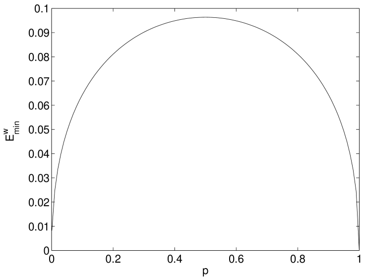
Figure 2: Residual squared error $E_{min}^{w}$ (38) as a function of $p$, the prior probability of ${|\phi_{1}\rangle}$, when using a WLSM. The weights are chosen as $w_{1}=\sqrt{p}$ and $w_{2}=\sqrt{1-p}$. For $p=1/2$ the WLSM and the LSM coincide.

Suppose now we are given the additional information $p_{1}=p$ and $p_{2}=1-p$, where $p_{1}$ and $p_{2}$ denote the prior probabilities of ${|\phi_{1}\rangle}$ and ${|\phi_{2}\rangle}$ respectively, and $p\in(0,1)$. We may still employ the LSM to distinguish between the two states. However, we expect that a smaller residual squared error may be achieved by employing a WLSM. In Fig. 2 we plot the residual squared error $E_{min}^{w}$ given by (38) as a function of $p$, when using a WLSM with weights $w_{1}=\sqrt{p}$ and $w_{2}=\sqrt{1-p}$ (we will justify this choice of weights in Section 7). When $p=1/2$, $w_{1}=w_{2}$ and the resulting WLSM is equivalent to the LSM. For $p\neq 1/2$, the WLSM does indeed yield a smaller residual squared error than the LSM (for which the residual squared error is approximately $0.095$).

7 Comparison With Other Proposed Measurements

We now compare our results with the SRM proposed by Hausladen et al. in [10], and with the measurement proposed by Peres and Wootters in [11].

Hausladen et al. construct a POVM consisting of rank-one operators $\Pi_{i}={|\mu_{i}\rangle}{\langle\mu_{i}|}$ to distinguish between an arbitrary set of vectors ${|\phi_{i}\rangle}\,$. We refer to this POVM as the SRM. They give two alternative definitions of their measurement: Explicitly,

$$\overline{M}=((\Phi\Phi^{*})^{1/2})^{\dagger}\Phi,$$ (48)

where $\overline{M}$ denotes the matrix of columns ${|\overline{\mu}_{i}\rangle}$. Implicitly, the optimal measurement vectors ${|\overline{\mu_{i}}\rangle}$ are those that satisfy

$$S^{1/2}=\{{\langle\overline{\mu}_{j}|\phi_{k}\rangle}\},$$ (49)

i.e., ${\langle\overline{\mu}_{j}|\phi_{k}\rangle}$ is equal to the $jk$th element of $S^{1/2}$, where $S=\Phi^{*}\Phi$.

Comparing (48) with (17), it is evident that the SRM coincides with the optimal LSM. Furthermore, following the discussion in Section 4, if the states are linearly independent then this measurement is a simple orthogonal measurement and not a more general POVM. (This observation was made in [13] as well.)

The implicit definition of (49) does not have a unique solution when the vectors ${|\phi_{i}\rangle}\,$are linearly dependent. The columns of $\overline{M}$ are one solution of this equation. Since the definition depends only on the product $M^{*}\Phi$, any measurement vectors that are columns of $M$ such that $M^{*}\Phi=\overline{M}^{*}\Phi$ constitutes a solution as well. In particular, the optimal orthogonal LSM $\tilde{M}$ for the linearly dependent case, given by (22), satisfies $\tilde{M}^{*}\Phi=\overline{M}^{*}\Phi$, rendering the optimal orthogonal LSM a solution to (49). Consequently, even in the case of linearly dependent states, the SRM proposed by Hausladen et al. and used to achieve the classical capacity of a quantum channel may always be chosen as an orthogonal measurement. In addition, this measurement is optimal in the least-squares sense.

We summarize our results regarding the SRM in the following theorem:

Theorem 3 (Square-root measurement (SRM))

Let $\{{|\phi_{i}\rangle}\}$ be a set of $m$ vectors in an $n$-dimensional complex Hilbert space ${\mathcal{H}}$ that span an $r$-dimensional subspace ${\mathcal{U}}\subseteq{\mathcal{H}}$. Let $\Phi=U\Sigma V^{*}$ be the rank-$r$ $n\times m$ matrix whose columns are the vectors ${|\phi_{i}\rangle}$. Let ${|u_{i}\rangle}$ and ${|v_{i}\rangle}$ denote the columns of the unitary matrices $U$ and $V$ respectively, and let $Z_{r}$ be defined as in (13). Let $\{{|\overline{\mu}_{i}\rangle}\}$ be $m$ vectors satisfying

$$S^{1/2}=\{{\langle\overline{\mu}_{j}|\phi_{k}\rangle}\},$$

where $S=\Phi^{*}\Phi$; a POVM consisting of the operators $\overline{\Pi}_{i}={|\overline{\mu}_{i}\rangle}{\langle\overline{\mu}_{i}|},\,1\leq i\leq m$, is referred to as a SRM. Let $\overline{M}$ be the $n\times m$ measurement matrix whose columns are the vectors ${|\overline{\mu}_{i}\rangle}$; $\overline{M}$ is referred to as a SRM matrix. Then

1. If $r=m$,

   1. $\overline{M}=\sum_{i=1}^{m}{|u_{i}\rangle}{\langle v_{i}|}=UZ_{m}V^{*}=\Phi(\Phi^{*}\Phi)^{-1/2}=((\Phi\Phi^{*})^{1/2})^{\dagger}\Phi$ is unique;

   2. $\overline{M}^{*}\overline{M}=I_{m}$ and the corresponding SRM is an orthogonal measurement;

   3. the SRM is equal to the optimal LSM.

2. If $r<m$,

   1. the SRM is not unique;

   2. $\overline{M}=\sum_{i=1}^{m}{|u_{i}\rangle}{\langle v_{i}|}=UZ_{m}V^{*}$ is a SRM matrix; the corresponding SRM is equal to the optimal orthogonal LSM;

   3. define $\overline{M}_{\mathcal{U}}=P_{\mathcal{U}}\overline{M}$, where $P_{\mathcal{U}}$ is a projection onto ${\mathcal{U}}$ and $\overline{M}$ is any SRM matrix; then

      1. $\overline{M}_{\mathcal{U}}$ is unique, and is given by $\overline{M}_{\mathcal{U}}=\sum_{i=1}^{r}{|u_{i}\rangle}{\langle v_{i}|}=UZ_{r}V^{*}=\Phi((\Phi^{*}\Phi)^{1/2})^{\dagger}=((\Phi\Phi^{*})^{1/2})^{\dagger}\Phi$;

      2. $\overline{M}_{\mathcal{U}}$ is a SRM matrix; the corresponding SRM is equal to the optimal LSM.

      3. $\overline{M}_{\mathcal{U}}$ may be realized by the optimal orthogonal LSM $\tilde{M}=\sum_{i=1}^{m}{|u_{i}\rangle}{\langle v_{i}|}=UZ_{m}V^{*}=\overline{M}$.

The SRM defined in [10] does not take the prior probabilities of the states ${|\phi_{i}\rangle}\,$into account. In [9], a more general definition of the SRM that accounts for the prior probabilities is given by defining new vectors ${|\phi_{i}^{w}\rangle}=\sqrt{p_{i}}{|\phi_{i}\rangle}$. The weighted SRM (WSRM) is then defined as the SRM corresponding to the vectors ${|\phi_{i}^{w}\rangle}$. Similarly, the WLSM is equal to the LSM corresponding to the vectors $w_{i}{|\phi_{i}\rangle}$. Thus, if we choose the the weights $w_{i}$ proportional to $\sqrt{p_{i}}$, then the WLSM coincides with the WSRM. A theorem similar to Theorem 3 may then be formulated where the WSRM and the WLSM are substituted for the SRM and the LSM.

We next apply our results to a problem considered by Peres and Wootters in [11]. The problem is to distinguish between three two-qubit states

$${|\phi_{1}\rangle}={|aa\rangle},\,\,{|\phi_{2}\rangle}={|bb\rangle},\,\,{|\phi_{3}\rangle}={|cc\rangle},$$ (50)

where ${|a\rangle},{|b\rangle}$ and ${|c\rangle}$ correspond to polarizations of a photon at $0^{\circ},60^{\circ}$ and $120^{\circ}$, and the states have equal prior probabilities. Since the vectors ${|\phi_{i}\rangle}\,$are linearly independent, the optimal measurement vectors are the columns of $\hat{M}\,$given by (16),

$$\hat{M}=\Phi(\Phi^{*}\Phi)^{-1/2}.$$ (51)

Substituting (50) in (51) results in the same measurement vectors ${|\hat{\mu}_{i}\rangle}$ as those proposed by Peres and Wootters. Thus their measurement is optimal in the least-squares sense. Furthermore, the measurement that they propose coincides with the SRM for this case. In the next section we will show that this measurement also minimizes the probability of a detection error.

8 The SRM for Geometrically Uniform State Sets

In this section we will consider the case in which the collection of states has a strong symmetry property, called geometric uniformity [16]. Under these conditions we show that the SRM is equivalent to the measurement minimizing the probability of a detection error, which we refer to as the MPEM. This result generalizes a similar result of Ban et al. [7].

8.1 Geometrically Uniform State Sets

Let ${\mathcal{G}}$ be a finite abelian (commutative) group of $m$ unitary matrices $U_{i}$. That is, ${\mathcal{G}}$ contains the identity matrix $I$; if ${\mathcal{G}}$ contains $U_{i}$, then it also contains its inverse $U_{i}^{-1}=U_{i}^{*}$; the product $U_{i}U_{j}$ of any two elements of ${\mathcal{G}}$ is in ${\mathcal{G}}$; and $U_{i}U_{j}=U_{j}U_{i}$ for any two elements in ${\mathcal{G}}$ [19].

A state set generated by ${\mathcal{G}}$ is a set ${\mathcal{S}}=\{{|\phi_{i}\rangle}=U_{i}{|\phi\rangle},U_{i}\in{\mathcal{G}}\}$, where ${|\phi\rangle}$ is an arbitrary state. The group ${\mathcal{G}}$ will be called the generating group of ${\mathcal{S}}$. Such a state set has strong symmetry properties, and will be called geometrically uniform (GU). For consistency with the symmetry of ${\mathcal{S}}$, we will assume equiprobable prior probabilities on ${\mathcal{S}}$.

If the group ${\mathcal{G}}$ contains a rotation $R$ such that $R^{k}=I$ for some integer $k>1$, then the GU state set ${\mathcal{S}}$ is linearly dependent, because $\sum_{j=1}^{k}R^{j}{|\phi\rangle}$ is a fixed point under $R$, and the only fixed point of a rotation is the zero vector ${|0\rangle}$.

Since $U_{i}^{*}=U_{i}^{-1}$, the inner product of two vectors in ${\mathcal{S}}$ is

$${\langle\phi_{i}|\phi_{j}\rangle}={\langle\phi|}U_{i}^{-1}U_{j}{|\phi\rangle}=s(U_{i}^{-1}U_{j}),$$ (52)

where $s$ is the function on ${\mathcal{G}}$ defined by

$$s(U_{i})={\langle\phi|}U_{i}{|\phi\rangle}.$$ (53)

For fixed $i$, the set $U_{i}^{-1}{\mathcal{G}}=\{U_{i}^{-1}U_{j},U_{j}\in{\mathcal{G}}\}$ is just a permutation of ${\mathcal{G}}$ since $U_{i}^{-1}U_{j}\in{\mathcal{G}}$ for all $i,j$ [19]. Therefore the $m$ numbers $\{s(U_{i}^{-1}U_{j}),1\leq j\leq m\}$ are a permutation of the numbers $\{s(U_{i}),1\leq i\leq m\}$. The same is true for fixed $j$. Consequently, every row and column of the $m\times m$ Gram matrix $S=\{{\langle\phi_{i}|\phi_{j}\rangle}\}$ is a permutation of the numbers $\{s(U_{i}),1\leq i\leq m\}$.

It will be convenient to replace the multiplicative group ${\mathcal{G}}$ by an additive group $G$ to which ${\mathcal{G}}$ is isomorphic. Every finite abelian group ${\mathcal{G}}$ is isomorphic to a direct product $G$ of a finite number of cyclic groups: ${\mathcal{G}}\cong G={\mathbb{Z}}_{m_{1}}\times\cdots\times{\mathbb{Z}}_{m_{p}}$, where ${\mathbb{Z}}_{m_{k}}$ is the cyclic additive group of integers modulo $m_{k}$, and $m=\prod_{k}m_{k}$ [19]. Thus every element $U_{i}\in{\mathcal{G}}$ can be associated with an element $g\in G$ of the form $g=(g_{1},g_{2},\ldots,g_{p})$, where $g_{k}\in{\mathbb{Z}}_{m_{k}}$. We denote this one-to-one correspondence by $U_{i}\leftrightarrow g$. Because the correspondence is an isomorphism, it follows that if $U_{i}\leftrightarrow g,\,U_{k}\leftrightarrow g^{\prime},\,U_{l}\leftrightarrow g^{\prime\prime}$ and $U_{i}=U_{k}U_{l}$, then $g=g^{\prime}+g^{\prime\prime}$, where the addition of $g^{\prime}=(g^{\prime}_{1},g^{\prime}_{2},\ldots,g^{\prime}_{p})$ and $g^{\prime\prime}=(g^{\prime\prime}_{1},g^{\prime\prime}_{2},\ldots,g^{\prime\prime}_{p})$ is performed by componentwise addition modulo the corresponding $m_{k}$.

Each state vector ${|\phi_{i}\rangle}=U_{i}{|\phi\rangle}$ will henceforth be denoted as ${|\phi(g)\rangle}$, where $g\in G$ is the group element corresponding to $U_{i}\in{\mathcal{G}}$. The zero element $0=(0,0,\ldots,0)\in G$ corresponds to the identity matrix $I\in{\mathcal{G}}$, and an additive inverse $-g\in G$ corresponds to a multiplicative inverse $U_{i}^{-1}=U_{i}^{*}\in{\mathcal{G}}$. The Gram matrix is then the $m\times m$ matrix

$$S=\{{\langle\phi(g^{\prime})|\phi(g)\rangle},g^{\prime},g\in G\}=\{s(g-g^{\prime}),g^{\prime},g\in G\},$$ (54)

with row and column indices $g^{\prime},g\in G$, where $s$ is now the function on $G$ defined by

$$s(g)={\langle\phi(0)|\phi(g)\rangle}.$$ (55)

8.2 The SRM

We now obtain the SRM for a GU state set. We begin by determining the SVD of $\Phi$. To this end we introduce the following definition. The Fourier transform (FT) of a complex-valued function $\varphi:G\to{\mathbb{C}}$ defined on $G={\mathbb{Z}}_{m_{1}}\times\cdots\times{\mathbb{Z}}_{m_{p}}$ is the complex-valued function $\hat{\varphi}:G\to{\mathbb{C}}$ defined by

$$\hat{\varphi}(h)=\frac{1}{\sqrt{m}}\sum_{g\in G}\langle{h},{g}\rangle\varphi(g),$$ (56)

where the Fourier kernel $\langle{h},{g}\rangle$ is

$$\langle{h},{g}\rangle=\prod_{k=1}^{p}e^{-2\pi ih_{k}g_{k}/m_{k}}.$$ (57)

Here $h_{k}$ and $g_{k}$ are the $k$th components of $h$ and $g$ respectively, and the product $h_{k}g_{k}$ is taken as an ordinary integer modulo $m_{k}$. The Fourier kernel evidently satisfies:

$$\langle{h},{g}\rangle = \langle{g},{h}\rangle;$$ (58)

$$\langle{h},{g}\rangle^{*} = \langle{-h},{g}\rangle=\langle{h},{-g}\rangle;$$ (59)

$$\langle{h+h^{\prime}},{g}\rangle = \langle{h},{g}\rangle\langle{h^{\prime}},{g}\rangle;$$ (60)

$$\langle{h},{g+g^{\prime}}\rangle = \langle{h},{g}\rangle\langle{h},{g^{\prime}}\rangle.$$ (61)

We define the FT matrix over $G$ as the $m\times m$ matrix ${\mathcal{F}}=\{\frac{1}{\sqrt{m}}\langle{h},{g}\rangle,h,g\in G\}$. The FT of a column vector ${|\varphi\rangle}=\{\varphi(g),g\in G\}$ is then the column vector ${|\hat{\varphi}\rangle}=\{\hat{\varphi}(h),h\in G\}$ given by ${|\hat{\varphi}\rangle}={\mathcal{F}}{|\varphi\rangle}$. It is easy to show that the rows and columns of ${\mathcal{F}}$ are orthonormal; i.e., ${\mathcal{F}}$ is unitary:

$${\mathcal{F}}^{*}{\mathcal{F}}={\mathcal{F}}{\mathcal{F}}^{*}=I_{m}.$$ (62)

Consequently we obtain the inverse FT formula

$${|\varphi\rangle}={\mathcal{F}}^{*}{|\hat{\varphi}\rangle}=\left\{\frac{1}{\sqrt{m}}\sum_{h\in G}\langle{h},{g}\rangle^{*}\hat{\varphi}(h),g\in G\right\}.$$ (63)

We now show that the eigenvectors of the Gram matrix $S$ of (54) are the column vectors ${|{\mathcal{F}}(h)\rangle}=\{\frac{1}{\sqrt{m}}\langle{h},{g}\rangle,g\in G\}$ of ${\mathcal{F}}$. Let ${\langle S(g^{\prime})|}=\{s(g-g^{\prime}),g\in G\}$ be the $g^{\prime}$th row of $S$. Then

$${\langle S(g^{\prime})|{\mathcal{F}}(h)\rangle}=\frac{1}{\sqrt{m}}\sum_{g\in G}\langle{h},{g}\rangle s(g-g^{\prime})=\frac{1}{\sqrt{m}}\sum_{g^{\prime\prime}\in G}\langle{h},{g^{\prime}+g^{\prime\prime}}\rangle s(g^{\prime\prime})=\langle{h},{g^{\prime}}\rangle\hat{s}(h),$$ (64)

where the last equality follows from (61), and $\{\hat{s}(h),h\in G\}$ is the FT of $\{s(g),g\in G\}$. Thus $S$ has the eigendecomposition

$$S={\mathcal{F}}\overline{\Sigma}^{2}{\mathcal{F}}^{*},$$ (65)

where $\overline{\Sigma}$ is an $m\times m$ diagonal matrix with diagonal elements $\{\sigma(h)=m^{1/4}\sqrt{\hat{s}(h)},h\in G\}$ (the eigenvalues $\sigma^{2}(h)$ are real and nonnegative because $S$ is Hermitian). Consequently, the $V$-basis of the SVD of $\Phi$ is $V={\mathcal{F}}$, and the singular values of $\Phi$ are $\sigma(h)$.

We now write the SVD of $\Phi$ in the following form:

$$\Phi=\Upsilon\overline{\Sigma}{\mathcal{F}}^{*}=\sum_{h\in G}\sigma(h){|u(h)\rangle}{\langle{\mathcal{F}}^{*}(h)|},$$ (66)

where $\Upsilon$ is the $n\times m$ matrix whose columns ${|u(h)\rangle}$ are the columns of the $U$-basis of the SVD of $\Phi$ for values of $h\in G$ such that $\sigma(h)\neq 0$ and are zero columns otherwise, and ${\mathcal{F}}^{*}=\{\frac{1}{\sqrt{m}}\langle{h},{g}\rangle^{*},h,g\in G\}$ has rows ${\langle{\mathcal{F}}^{*}(h)|}=\{\frac{1}{\sqrt{m}}\langle{h},{g}\rangle^{*},g\in G\}$. It then follows that

$${|u(h)\rangle} = \left\{\begin{array}[]{ll}\Phi{|{\mathcal{F}}(h)\rangle}/\sigma(h)={|\hat{\phi}(h)\rangle}/\sigma(h),&\mbox{if}\,\,\sigma(h)\neq 0;\\ {|0\rangle},&\mathrm{otherwise,}\end{array}\right.$$ (69)

where

$${|\hat{\phi}(h)\rangle}=\frac{1}{\sqrt{m}}\sum_{g\in G}\langle{h},{g}\rangle{|\phi(g)\rangle}$$ (70)

is the $h$th element of the FT of $\Phi$ regarded as a row vector of column vectors, $\Phi=\{{|\phi(g)\rangle},g\in G\}$.

Finally, the SRM is given by the measurement matrix

$$M=\Upsilon{\mathcal{F}}^{*}=\sum_{h\in G}{|u(h)\rangle}{\langle{\mathcal{F}}^{*}(h)|}.$$ (71)

The measurement vectors ${|\mu(g)\rangle}$ (the columns of $M$) are thus the inverse FT of the columns of $\Upsilon$:

$${|\mu(g)\rangle}=\frac{1}{\sqrt{m}}\sum_{h\in G}\langle{g},{h}\rangle^{*}{|u(h)\rangle}.$$ (72)

Note that if ${|\phi(g)\rangle}=U_{i}{|\phi\rangle}$ where $U_{i}\leftrightarrow g$, and $U_{j}\leftrightarrow g^{\prime}$, then $U_{j}{|\phi(g)\rangle}=U_{j}U_{i}{|\phi\rangle}={|\phi(g+g^{\prime})\rangle}$. Therefore left multiplication of the state vectors $\Phi=\{{|\phi(g)\rangle},g\in G\}$ by $U_{j}$ permutes the state vectors to $U_{j}\Phi=\{{|\phi(g+g^{\prime})\rangle},g\in G\}$. We now show that under this transformation the measurement vectors are similarly permuted; i.e., $U_{j}M=\{{|\mu(g+g^{\prime})\rangle},g\in G\}$. The FT of the permuted vectors $\{{|\phi(g+g^{\prime})\rangle},g\in G\}$ is

$${|\hat{\phi^{\prime}}(h)\rangle}=\frac{1}{\sqrt{m}}\sum_{g\in G}\langle{h},{g}\rangle{|\phi(g+g^{\prime})\rangle}=\frac{1}{\sqrt{m}}\sum_{g^{\prime\prime}\in G}\langle{h},{g^{\prime\prime}-g^{\prime}}\rangle{|\phi(g^{\prime\prime})\rangle}=\langle{h},{g^{\prime}}\rangle^{*}{|\hat{\phi}(h)\rangle}.$$ (73)

Normalization by $\sigma(h)^{-1}$ when $\sigma(h)\neq 0$ yields ${|u^{\prime}(h)\rangle}=\langle{h},{g^{\prime}}\rangle^{*}{|u(h)\rangle}$. Finally, the inverse FT yields the measurement vectors

$${|\mu^{\prime}(g)\rangle}=\frac{1}{\sqrt{m}}\sum_{h\in G}\langle{g},{h}\rangle^{*}{|u^{\prime}(h)\rangle}=\frac{1}{\sqrt{m}}\sum_{h\in G}\langle{g+g^{\prime}},{h}\rangle^{*}{|u(h)\rangle}={|\mu(g+g^{\prime})\rangle},$$ (74)

where we have used (58) and (60).

This shows that the measurement vectors ${|\mu(g)\rangle}$ have the same symmetries as the state vectors; i.e., they also form a GU set with generating group ${\mathcal{G}}$. Explicitly, if $U_{i}\leftrightarrow g$, then ${|\mu(g)\rangle}=U_{i}{|\mu\rangle}$, where ${|\mu\rangle}$ denotes ${|\mu(0)\rangle}$.

8.3 The SRM and the MPEM

We now show that for GU state sets the SRM is equivalent to the MPEM. In the process, we derive a sufficient condition for the SRM to minimize the probability of a detection error for a general state set (not necessarily GU) comprised of linearly independent states.

Holevo [2, 4] and Yuen et al. [3] showed that a set of measurement operators $\Pi_{i}$ comprises the MPEM for a set of weighted density operators $W_{i}=p_{i}\rho_{i}$ if they satisfy

$$\Pi_{i}(W_{j}-W_{i})\Pi_{j} = {\mathbf{0}},\,\,\forall g,g^{\prime};$$ (75)

$$\Gamma-W_{i} \geq {\mathbf{0}},\,\,\forall g,$$ (76)

where

$$\Gamma=\sum_{j=1}^{m}\Pi_{j}W_{j}$$ (77)

and is required to be Hermitian. Note that if (75) is satisfied, then $\Gamma$ is Hermitian.

In our case the measurement operators $\Pi_{i}$ are the operators ${|\mu(g)\rangle}{\langle\mu(g)|}$, and the weighted density operators may be taken simply as the projectors ${|\phi(g)\rangle}{\langle\phi(g)|}$, since their prior probabilities are equal. The conditions (75)-(76) then become

$${|\mu(g)\rangle}{\langle\mu(g)|\phi(g^{\prime})\rangle}{\langle\phi(g^{\prime})|\mu(g^{\prime})\rangle}{\langle\mu(g^{\prime})|}={|\mu(g)\rangle}{\langle\mu(g)|\phi(g)\rangle}{\langle\phi(g)|\mu(g^{\prime})\rangle}{\langle\mu(g^{\prime})|},\,\,\forall g,g^{\prime};$$ (78)

$$\sum_{g^{\prime}}{|\mu(g^{\prime})\rangle}{\langle\mu(g^{\prime})|\phi(g^{\prime})\rangle}{\langle\phi(g^{\prime})|}-{|\phi(g)\rangle}{\langle\phi(g)|}\geq{\mathbf{0}},\,\,\forall g.$$ (79)

We first verify that the conditions (75) (or equivalently (78)) are satisfied. Since the matrix $M^{*}\Phi={\mathcal{F}}\overline{\Sigma}{\mathcal{F}}^{*}$ is symmetric, ${\langle\mu(g^{\prime})|\phi(g)\rangle}={\langle\mu|}U_{j}^{-1}U_{i}{|\phi\rangle}=w(g-g^{\prime})$, where $w(g)={\langle\mu|\phi(g)\rangle}$ is a complex-valued function that satisfies $w(-g)=w^{*}(g)$. Therefore,

$${\langle\mu(g)|\phi(g^{\prime})\rangle} = w(g^{\prime}-g)=w^{*}(g-g^{\prime})={\langle\phi(g)|\mu(g^{\prime})\rangle};$$ (80)

$${\langle\phi(g^{\prime})|\mu(g^{\prime})\rangle} = w^{*}(0)=w(0)={\langle\mu(g)|\phi(g)\rangle}.$$ (81)

Substituting these relations back into (78), we obtain

$$w(0)w(g^{\prime}-g){|\mu(g)\rangle}{\langle\mu(g^{\prime})|}=w(0)w(g^{\prime}-g){|\mu(g)\rangle}{\langle\mu(g^{\prime})|},\,\,\forall g,g^{\prime},$$ (82)

which verifies that the conditions (75) are satisfied.

Next, we show that conditions (76) are satisfied. Since $M^{*}\Phi={\mathcal{F}}\overline{\Sigma}{\mathcal{F}}^{*}$,

$$w(0)={\langle\mu(g)|\phi(g)\rangle}={\langle{\mathcal{F}}(g)|}\overline{\Sigma}{|{\mathcal{F}}(g)\rangle},$$ (83)

where ${\langle{\mathcal{F}}(g)|}$ denotes the row of ${\mathcal{F}}$ corresponding to $g$. Then,

$$\Gamma=\sum_{g^{\prime}}{|\mu(g^{\prime})\rangle}{\langle\mu(g^{\prime})|\phi(g^{\prime})\rangle}{\langle\phi(g^{\prime})|}=w(0)\sum_{g^{\prime}}{|\mu(g^{\prime})\rangle}{\langle\phi(g^{\prime})|}.$$ (84)

From (66) and (71) we have

$$\sum_{g^{\prime}}{|\mu(g^{\prime})\rangle}{\langle\phi(g^{\prime})|}=\Upsilon\overline{\Sigma}\Upsilon^{*},$$ (85)

and

$${|\phi(g)\rangle}{\langle\phi(g)|}=\Upsilon\overline{\Sigma}{|{\mathcal{F}}(g)\rangle}{\langle{\mathcal{F}}(g)|}\overline{\Sigma}\Upsilon^{*}.$$ (86)

Substituting (84)-(86) back into (79), the conditions of (79) reduce to

$$\Upsilon\left(w(0)\overline{\Sigma}-\overline{\Sigma}{|{\mathcal{F}}(g)\rangle}{\langle{\mathcal{F}}(g)|}\overline{\Sigma}\right)\Upsilon^{*}\geq{\mathbf{0}},$$ (87)

where $w(0)$ is given by (83). It is therefore sufficient to show that

$$T=w(0)\overline{\Sigma}-\overline{\Sigma}{|{\mathcal{F}}(g)\rangle}{\langle{\mathcal{F}}(g)|}\overline{\Sigma}\geq{\mathbf{0}}$$ (88)

or equivalently that ${\langle u|T|u\rangle}\geq 0$ for any ${|u\rangle}\in{\mathbb{C}}^{m}$. Using the Cauchy-Schwartz inequality we have

$${\langle u|T|u\rangle} = {\langle{\mathcal{F}}(g)|}\overline{\Sigma}{|{\mathcal{F}}(g)\rangle}{\langle u|}\overline{\Sigma}{|u\rangle}-{\langle u|}\overline{\Sigma}{|{\mathcal{F}}(g)\rangle}{\langle{\mathcal{F}}(g)|}\overline{\Sigma}{|u\rangle}$$ (89)

$$\geq {\langle{\mathcal{F}}(g)|}\overline{\Sigma}{|{\mathcal{F}}(g)\rangle}{\langle u|}\overline{\Sigma}{|u\rangle}-{\langle{\mathcal{F}}(g)|}\overline{\Sigma}{|{\mathcal{F}}(g)\rangle}{\langle u|}\overline{\Sigma}{|u\rangle}=0,$$

which verifies that the conditions (76) are satisfied. We conclude that when the state set ${\mathcal{S}}$ is GU, the SRM is also the MPEM.

An alternative way of deriving this result for the case of linearly independent states ${|\phi_{i}\rangle}$ is by use of the following criterion of Sasaki et al. [13]. Denote by $\Phi_{w}$ the matrix whose columns are the vectors ${|\phi_{i}^{w}\rangle}=\sqrt{p_{i}}{|\phi_{i}\rangle}$ where $p_{i}$ is the prior probability of state $i$. If the states are linearly independent and $S^{1/2}=(\Phi_{w}^{*}\Phi_{w})^{1/2}$ has constant diagonal elements, then the SRM corresponding to the vectors ${|\phi_{i}^{w}\rangle}$ (i.e., a WSRM), is equivalent to the MPEM.

This condition is hard to verify directly from the vectors ${|\phi_{i}^{w}\rangle}$. The difficulty arises from the fact that generally there is no simple relation between the diagonal elements of $S^{1/2}$ and the elements of $S$. Thus given an ensemble of pure states ${|\phi_{i}\rangle}\,$with prior probabilities $p_{i}$, we typically need to calculate $S^{1/2}$ (which in itself is not simple to do analytically) in order to verify the condition above. However, as we now show, in some cases this condition may be verified directly from the elements of $S$ using the SVD.

Employing the SVD $\Phi_{w}=U\Sigma V^{*}$ we may express $S^{1/2}$ as

$$S^{1/2}=(\Phi_{w}^{*}\Phi_{w})^{1/2}=V(\Sigma^{*}\Sigma)^{1/2}V^{*}=V\overline{\Sigma}V^{*},$$ (90)

where $\overline{\Sigma}$ is a diagonal matrix with the first $r$ diagonal elements equal to $\sigma_{i}$, and the remaining elements all equal zero, where the $\sigma_{i}$ are the singular values of $\Phi_{w}$. Thus, the WSRM is equal to the MPEM if ${\langle\overline{v}_{i}|}\overline{\Sigma}{|\overline{v}_{i}\rangle}=c,\,\,1\leq i\leq m$, where the vectors ${|\overline{v}_{i}\rangle}$ denote the columns of $V^{*}$, and $c$ is a constant. In particular, if the elements of $V$ all have equal magnitude, then ${\langle\overline{v}_{i}|}\overline{\Sigma}{|\overline{v}_{i}\rangle}$ is constant, and the SRM minimizes the probability of a detection error.

If the state set ${\mathcal{S}}$ is GU, then the matrix $V$ is the FT matrix ${\mathcal{F}}$, whose elements all have magnitude equal to one. Thus, if the states are linearly independent and GU, then the SRM is equivalent to the MPEM.

We summarize our results regarding GU state sets in the following theorem:

Theorem 4 (SRM for GU state sets)

Let ${\mathcal{S}}=\{{|\phi_{i}\rangle}=U_{i}{|\phi\rangle},U_{i}\in{\mathcal{G}}\}$, be a geometrically uniform state set generated by a finite abelian group ${\mathcal{G}}$ of unitary matrices, where ${|\phi\rangle}$ is an arbitrary state. Let ${\mathcal{G}}\cong G$, and let $\Phi$ be the matrix of columns ${|\phi_{i}\rangle}$. Then the SRM is given by the measurement matrix

$$M=\Phi{\mathcal{F}}\overline{\Sigma}^{\dagger}{\mathcal{F}}^{*}=\sum_{h\in G}{|u(h)\rangle}{\langle{\mathcal{F}}^{*}(h)|},$$

where ${\mathcal{F}}$ is the Fourier transform matrix over $G$, $\overline{\Sigma}^{\dagger}$ is the diagonal matrix whose diagonal elements are $\sigma(h)^{-1}$ when $\sigma(h)\neq 0$ and $0$ otherwise, where $\{\sigma(h),h\in G\}$ are the singular values of $\Phi$, ${|u(h)\rangle}={|\hat{\phi}(h)\rangle}/\sigma(h)$ when $\sigma(h)\neq 0$ and ${|0\rangle}$ otherwise, where $\{{|\hat{\phi}(h)\rangle},h\in G\}$ is the Fourier transform of $\{{|\phi(g)\rangle},g\in G\}$, and ${\langle{\mathcal{F}}^{*}(h)|}$ is the $h$th row of ${\mathcal{F}}^{*}$.

The SRM has the following properties:

1. The measurement matrix $M$ has the same symmetries as $\Phi$;

2. The SRM is the least-squares measurement (LSM);

3. The SRM is the minimum-probability-of-error measurement (MPEM).

8.4 Example of a GU State Set

We now consider an example demonstrating the ideas of the previous section. Consider the group ${\mathcal{G}}$ of $m=4$ unitary matrices $U_{i}$, where

$$U_{1}=I_{4},\,\,\,U_{2}=\left[\begin{array}[]{rrrr}-1&0&0&0\\ 0&1&0&0\\ 0&0&-1&0\\ 0&0&0&-1\end{array}\right],\,\,\,U_{3}=\left[\begin{array}[]{rrrr}-1&0&0&0\\ 0&-1&0&0\\ 0&0&1&0\\ 0&0&0&-1\end{array}\right],\,\,\,U_{4}=U_{2}U_{3}.$$ (91)

Let the state set be ${\mathcal{S}}=\{{|\phi_{i}\rangle}=U_{i}{|\phi\rangle},\,\,1\leq i\leq 4\}$, where ${|\phi\rangle}=\frac{1}{2}[1\,\,1\,\,1\,\,1]^{*}$. Then $\Phi$ is

$$\Phi=\frac{1}{2}\left[\begin{array}[]{rrrr}1&-1&-1&1\\ 1&1&-1&-1\\ 1&-1&1&-1\\ 1&-1&-1&1\end{array}\right],$$ (92)

and the Gram matrix $S$ is given by

$$S=\frac{1}{2}\left[\begin{array}[]{rrrr}2&-1&-1&0\\ -1&2&0&-1\\ -1&0&2&-1\\ 0&-1&-1&2\end{array}\right].$$ (93)

Note that the sum of the states ${|\phi_{i}\rangle}$ is ${|0\rangle}$, so the state set is linearly dependent.

In this case ${\mathcal{G}}$ is isomorphic to $G={\mathbb{Z}}_{2}\times{\mathbb{Z}}_{2}$, i.e., $G=\{(0,0),(0,1),(1,0),(1,1)\}$. The multiplication table of the group ${\mathcal{G}}$ is

$$\begin{array}[]{c|cccc}&U_{1}&U_{2}&U_{3}&U_{4}\\ \hline\cr U_{1}&U_{1}&U_{2}&U_{3}&U_{4}\\ U_{2}&U_{2}&U_{1}&U_{4}&U_{3}\\ U_{3}&U_{3}&U_{4}&U_{1}&U_{2}\\ U_{4}&U_{4}&U_{3}&U_{2}&U_{1}.\end{array}$$ (94)

If we define the correspondence

$$U_{1}\leftrightarrow(0,0),\,\,U_{2}\leftrightarrow(0,1),\,\,U_{3}\leftrightarrow(1,0),\,\,U_{4}\leftrightarrow(1,1),$$ (95)

then this table becomes the addition table of $G={\mathbb{Z}}_{2}\times{\mathbb{Z}}_{2}$:

$$\begin{array}[]{c|cccc}&(0,0)&(0,1)&(1,0)&(1,1)\\ \hline\cr(0,0)&(0,0)&(0,1)&(1,0)&(1,1)\\ (0,1)&(0,1)&(0,0)&(1,1)&(1,0)\\ (1,0)&(1,0)&(1,1)&(0,0)&(0,1)\\ (1,1)&(1,1)&(1,0)&(0,1)&(0,0).\end{array}$$ (96)

Only the way in which the elements are labeled distinguishes the table of (96) from the table of (94); thus ${\mathcal{G}}\cong G$. Comparing (94) and (96) with (93), we see that the tables and the matrix $S$ have the same symmetries.

Over $G={\mathbb{Z}}_{2}\times{\mathbb{Z}}_{2}$, the Fourier matrix ${\mathcal{F}}$ is the Hadamard matrix

$${\mathcal{F}}=\frac{1}{2}\left[\begin{array}[]{rrrr}1&1&1&1\\ 1&-1&1&-1\\ 1&1&-1&-1\\ 1&-1&-1&1\end{array}\right].$$ (97)

Using (69) and (71), we may find the measurement matrix of the SRM:

$$M=\frac{1}{2\sqrt{2}}\left[\begin{array}[]{rrrr}1&-1&-1&1\\ \sqrt{2}&\sqrt{2}&-\sqrt{2}&-\sqrt{2}\\ \sqrt{2}&-\sqrt{2}&\sqrt{2}&-\sqrt{2}\\ 1&-1&-1&1\end{array}\right].$$ (98)

We verify that the columns ${|\mu_{i}\rangle}$ of $M$ may be expressed as ${|\mu_{i}\rangle}=U_{i}{|\mu_{1}\rangle},\,\,1\leq i\leq 4$, where ${|\mu_{1}\rangle}=\frac{1}{2\sqrt{2}}[1\,\,\sqrt{2}\,\,\sqrt{2}\,\,1]^{*}$. Thus the measurement vectors ${|\mu_{i}\rangle}$ also form a GU set generated by ${\mathcal{G}}$.

8.5 Applications of GU State Sets

We now discuss some applications of Theorem 4.

A. Binary state set: Any binary state set ${\mathcal{S}}=\{{|\phi_{1}\rangle},{|\phi_{2}\rangle}\}$ is GU, because it can be generated by the binary group ${\mathcal{G}}=\{I,R\}$, where $I$ is the identity and $R$ is the reflection about the hyperplane halfway between the two states. Specifically, if the two states ${|\phi_{1}\rangle}$ and ${|\phi_{2}\rangle}$ are real, then

$$R=I-2\frac{{|w\rangle}{\langle w|}}{{\langle w|w\rangle}},$$ (99)

where ${|w\rangle}={|\phi_{2}\rangle}-{|\phi_{1}\rangle}$. We may immediately verify that $R^{2}=I$, so that $R^{-1}=R$, and that ${|\phi_{2}\rangle}=R{|\phi_{1}\rangle}$.

If the states are complex with ${\langle\phi_{1}|\phi_{2}\rangle}=ae^{j\theta}$, then define ${|\phi_{2}^{\prime}\rangle}=e^{-j\theta}{|\phi_{2}\rangle}$. The states ${|\phi_{2}\rangle}$ and ${|\phi_{2}^{\prime}\rangle}$ differ by a phase factor and therefore correspond to the same physical state. We may therefore replace our state set ${\mathcal{S}}=\{{|\phi_{1}\rangle},{|\phi_{2}\rangle}\}$ by the equivalent state set ${\mathcal{S}}=\{{|\phi_{1}\rangle},{|\phi_{2}^{\prime}\rangle}\}$. Now the generating group is ${\mathcal{G}}=\{I,R\}$, where $R$ is defined by (99), with ${|w\rangle}={|\phi_{2}^{\prime}\rangle}-{|\phi_{1}\rangle}$.

The generating group ${\mathcal{G}}=\{I,R\}$ is isomorphic to $G={\mathbb{Z}}_{2}$. The Fourier matrix ${\mathcal{F}}$ therefore reduces to the $2\times 2$ discrete FT (DFT) matrix,

$${\mathcal{F}}=\frac{1}{\sqrt{2}}\left[\begin{array}[]{rr}1&1\\ 1&-1\end{array}\right].$$ (100)

The squares of the singular values of $\Phi$ are therefore $\{\sigma^{2}(h)=\sqrt{2}\hat{s}(h),h\in G\}$ where $\{\hat{s}(h),h\in G\}$ are the DFT values of $\{s(g),g\in G\}$, with $s(0)=1$ and $s(1)=a$. Thus,

$$\sigma^{2}(0)=1+a;$$

$$\sigma^{2}(1)=1-a.$$ (101)

From Theorem 4 we then have

$$M=\Phi{\mathcal{F}}\overline{\Sigma}^{\dagger}{\mathcal{F}}^{*}=\frac{1}{2}\Phi\left[\begin{array}[]{rr}\frac{1}{\sigma(0)}+\frac{1}{\sigma(1)}&\frac{1}{\sigma(0)}-\frac{1}{\sigma(1)}\\ \frac{1}{\sigma(0)}-\frac{1}{\sigma(1)}&\frac{1}{\sigma(0)}+\frac{1}{\sigma(1)}\end{array}\right].$$ (102)

We may now apply (102) to the example of Section 6. In that example $a={\langle\phi_{1}|\phi_{2}\rangle}=-1/2$. From (8.5) it then follows that $\sigma(0)=1/\sqrt{2}$ and $\sigma(1)=\sqrt{3/2}$. Substituting these values in (102) yields

$$M=\Phi\left[\begin{array}[]{rr}1.12&0.30\\ 0.30&1.12\end{array}\right],$$ (103)

which is equivalent to the optimal measurement matrix obtained in Section 6.

We could have obtained the measurement vectors directly from the symmetry property of Theorem 4.1. The state set ${\mathcal{S}}=\{{|\phi_{1}\rangle},{|\phi_{2}\rangle}\}$ is invariant under a reflection about the line halfway between the two states, as illustrated in Fig. 3. The measurement vectors must also be invariant under the same reflection. In addition, since the states are linearly independent, the measurement vectors must be orthonormal. This completely determines the measurement vectors shown in Fig. 3. (The only other possibility, namely the negatives of these two vectors, is physically equivalent.)

B. Cyclic state set: A cyclic generating group ${\mathcal{G}}$ has elements $U_{i}=Q^{i-1},1\leq i\leq m$, where $Q$ is a unitary matrix with $Q^{m}=I$. A cyclic group generates a cyclic state set ${\mathcal{S}}=\{{|\phi_{i}\rangle}=Q^{i-1}{|\phi\rangle},\,\,1\leq i\leq m\}$, where ${|\phi\rangle}$ is arbitrary. Ban et al. [7] refer to such a cyclic state set as a symmetrical state set, and show that in that case the SRM is equivalent to the MPEM. This result is a special case of Theorem 4.

Using Theorem 4 we may obtain the measurement matrix $M$ as follows. If ${\mathcal{G}}$ is cyclic, then $S$ is a circulant matrix, and $G$ is the cyclic group ${\mathbb{Z}}_{m}$. The FT kernel is then $\langle{h},{g}\rangle=e^{-2\pi ihg/m}$ for $h,g\in{\mathbb{Z}}_{m}$, and the Fourier matrix ${\mathcal{F}}$ reduces to the $m\times m$ DFT matrix. The singular values of $\Phi$ are $m^{1/4}$ times the square roots of the DFT values of the inner products $\{{\langle\phi_{1}|\phi_{j}\rangle},1\leq j\leq m\}$. We then calculate $M=\Phi{\mathcal{F}}\overline{\Sigma}^{\dagger}{\mathcal{F}}^{*}$.

C. Peres-Wootters measurement: We may apply these results to the Peres-Wootters problem considered at the end of Section 7. In this problem the states to be distinguished are given by ${|\phi_{1}\rangle}={|aa\rangle},{|\phi_{2}\rangle}={|bb\rangle}$ and ${|\phi_{3}\rangle}={|cc\rangle}$, where ${|a\rangle},{|b\rangle}$ and ${|c\rangle}$ correspond to polarizations of a photon at $0^{\circ},60^{\circ}$ and $120^{\circ}$, and the states have equal prior probabilities. The state set ${\mathcal{S}}=\{{|\phi_{1}\rangle},{|\phi_{2}\rangle},{|\phi_{3}\rangle}\}$ is thus a cyclic state set with ${|\phi_{i}\rangle}=U_{i}{|\phi_{1}\rangle},1\leq i\leq 3$, where $U_{i}=(Q\otimes Q)^{i-1}$ and $Q$ is a rotation by $60^{\circ}$.

In Section 7 we concluded that the Peres-Wootters measurement is equivalent to the SRM and consequently minimizes the squared error. From Theorem 4 we now conclude that the Peres-Wootters measurement minimizes the probability of a detection error as well.

9 Conclusion

In this paper we constructed optimal measurements in the least-squares sense for distinguishing between a collection of quantum states. We considered POVMs consisting of rank-one operators, where the vectors were chosen to minimize a possibly weighted sum of squared errors. We saw that for linearly independent states the optimal least-squares measurement is an orthogonal measurement, which coincides with the SRM proposed by Hausladen et al. [10]. If the states are linearly dependent, then the optimal POVM still has the same general form. We showed that it may be realized by an orthogonal measurement of the same form as in the linearly independent case. We also noted that the SRM, which was constructed by Hausladen et al. [10] and used to achieve the classical channel capacity of a quantum channel, may always be chosen as an orthogonal measurement.

We showed that for a GU state set the SRM minimizes the probability of a detection error. We also derived a sufficient condition for the SRM to minimize the probability of a detection error in the case of linearly independent states based on the properties of the SVD.

Appendix A. Properties of the Residual Squared Error

We noted at the beginning of Section 3 that if the vectors ${|\phi_{i}\rangle}\,$are mutually orthonormal, then the optimal measurement is a set of projections onto the states ${|\phi_{i}\rangle}\,$, and the resulting squared error is zero. In this case $S=\Phi^{*}\Phi=I_{m}$, and $\sigma_{i}=1,\,\,1\leq i\leq m$.

If the vectors ${|\phi_{i}\rangle}\,$are normalized but not orthogonal, then we may decompose $S$ as $S=I_{m}+D$, where $D$ is the matrix of inner products ${\langle\phi_{i}|\phi_{j}\rangle}$ for $i\neq j$ and has diagonal elements all equal to $0$. We expect that if the inner products are relatively small, i.e., if the states ${|\phi_{i}\rangle}\,$are nearly orthonormal, then we will be able to distinguish between them pretty well; equivalently, we would expect the singular values to be close to $1$. Indeed, from [20] we have the following bound on the singular values of $S=I+D$:

$$|\sigma_{i}^{2}-1|^{2}\leq\mbox{Tr}(D^{*}D),\,\,\,1\leq i\leq m.$$ (104)

We now point out some properties of the minimal achievable squared error $E_{min}$ given by (15). For a given $m$, $E_{min}$ depends only on the singular values of the matrix $\Phi$. Consequently, any linear operation on the vectors ${|\phi_{i}\rangle}\,$that does not affect the singular values of $\Phi$ will not affect $E_{min}$.

For example, if we obtain a new set of states ${|\phi^{\prime}_{i}\rangle}$ by unitary mixing of the states ${|\phi_{i}\rangle}\,$, i.e., $\Phi^{\prime}=\Phi Q^{*}$ where $Q$ is an $m\times m$ unitary matrix, then the new optimal measurement vectors ${|\mu^{\prime}_{i}\rangle}$ will typically differ from the measurement vectors ${|\hat{\mu}_{i}\rangle}$; however the minimal achievable squared error is the same. Indeed, defining $S^{\prime}=\Phi^{\prime*}\Phi^{\prime}=QSQ^{*}$, where $S=\Phi^{*}\Phi$, we see that the matrices $S^{\prime}$ and $S$ are related through a similarity transformation and consequently have equal eigenvalues [20].

Next, suppose we obtain a new set of states ${|\phi^{\prime}_{i}\rangle}$ by a general nonsingular linear mixing of the states ${|\phi_{i}\rangle}$, i.e., $\Phi^{\prime}=\Phi A^{*}$, where $A$ is an arbitrary $m\times m$ nonsingular matrix. In this case the eigenvalues of $S^{\prime}=ASA^{*}$ will in general differ from the eigenvalues of $S$. Nevertheless, we have the following theorem:

Theorem 5

Let $E_{min}$ and $E^{\prime}_{min}$ denote the minimal achievable squared error when distinguishing between the pure state ensembles $\{{|\phi_{i}\rangle}\}$ and $\{{|\phi^{\prime}_{i}\rangle}\}$ respectively, where ${|\phi^{\prime}_{i}\rangle}=\sum_{j=1}^{m}a_{ij}^{*}{|\phi_{j}\rangle}$. Let $A$ denote the matrix whose $ij$th element is $a_{ij}$. Let $\lambda_{1}(AA^{*})$ and $\lambda_{m}(AA^{*})$ denote the largest and smallest eigenvalues of $AA^{*}$ respectively, and let $\{\sigma_{i},\,1\leq i\leq r\}$ denote the singular values of the matrix $\Phi$ of columns ${|\phi_{i}\rangle}\,$. Then,

$$2\left(1-\sqrt{\lambda_{1}(AA^{*})}\right)\sum_{i=1}^{r}\sigma_{i}\leq E^{\prime}_{min}-E_{min}\leq 2\left(1-\sqrt{\lambda_{m}(AA^{*})}\right)\sum_{i=1}^{r}\sigma_{i}.$$

Thus, $E^{\prime}_{min}\leq E_{min}$ if $\lambda_{m}(AA^{*})\geq 1$ and $E^{\prime}_{min}\geq E_{min}$ if $\lambda_{1}(AA^{*})\leq 1$.
In particular, if $A$ is unitary then $E_{min}=E^{\prime}_{min}$.

Proof: We rely on the following theorem due to Ostrowski (see e.g., [20], p. 224):

Ostrowski Theorem: Let $A$ and $S$ denote $m\times m$ matrices with $S$ Hermitian and $A$ nonsingular, and let $S^{\prime}=ASA^{*}$. Let $\lambda_{k}(\cdot)$ denote the $k$th eigenvalue of the corresponding matrix, where the eigenvalues are arranged in decreasing order. For every $1\leq i\leq m$, there exists a positive real number $a_{i}$ such that $\lambda_{m}(AA^{*})\leq a_{i}\leq\lambda_{1}(AA^{*})$ and $\lambda_{i}(S^{\prime})=a_{i}\lambda_{i}(S)$.

Combining this theorem with the expression (15) for the residual squared error results in $E^{\prime}_{min}-E_{min}=2\sum_{i=1}^{r}\left(1-\sqrt{a_{i}}\right)\sigma_{i}$. Substituting $\lambda_{m}(AA^{*})\leq a_{i}\leq\lambda_{1}(AA^{*})$ results in Theorem 5. If $A$ is unitary, then $AA^{*}=I$, and $\lambda_{i}(AA^{*})=1$ for all $i$.

Figure 1: $2$-dimensional example of the LSM. The state vectors ${|\phi_{1}\rangle}$ and ${|\phi_{2}\rangle}$ are given by (41), the optimal measurement vectors ${|\hat{\mu}_{1}\rangle}$ and ${|\hat{\mu}_{2}\rangle}$ are given by (45) and are orthonormal, and ${|e_{1}\rangle}$ and ${|e_{2}\rangle}$ denote the error vectors defined in (3).

Figure 3: Symmetry property of the state set ${\mathcal{S}}=\{{|\phi_{1}\rangle},{|\phi_{2}\rangle}\}$ and the optimum measurement vectors $\{{|\hat{\mu}_{1}\rangle},{|\hat{\mu}_{2}\rangle}\}$. ${|\phi_{1}\rangle}$ and ${|\phi_{2}\rangle}$ are given by (41), and ${|\hat{\mu}_{1}\rangle}$ and ${|\hat{\mu}_{2}\rangle}$ are given by (45). Because the state vectors are invariant under a reflection about the dashed line, the optimum measurement vectors must also have this property. In addition, the measurement vectors must be orthonormal. The symmetry and orthonormality properties completely determine the optimum measurement vectors $\{{|\hat{\mu}_{1}\rangle},{|\hat{\mu}_{2}\rangle}\}$ (up to sign reversal).

References

- [1] A. Peres, Quantum Theory: Concepts and Methods. Boston: Kluwer, 1995.
- [2] A. S. Holevo, “Statistical decisions in quantum theory,” J. Multivar. Anal., vol. 3, pp. 337-394, Dec. 1973.
- [3] H. P. Yuen, R. S. Kennedy and M. Lax, “Optimum testing of multiple hypotheses in quantum detection theory,” IEEE Trans. Inform. Theory, vol. IT-21, pp. 125-134, Mar. 1975.
- [4] C. W. Helstrom, Quantum Detection and Estimation Theory. New York: Academic Press, 1976.
- [5] M. Charbit, C. Bendjaballah and C. W. Helstrom, “Cutoff rate for the -ary PSK modulation channel with optimal quantum detection,” IEEE Trans. Inform. Theory, vol. 35, pp. 1131-1133, Sep. 1989.
- [6] M. Osaki, M. Ban and O. Hirota, “Derivation and physical interpretation of the optimum detection operators for coherent-state signals,” Phys. Rev. A, vol. 54, pp. 1691-1701, Aug. 1996.
- [7] M. Ban, K. Kurukowa, R. Momose and O. Hirota, “Optimum measurements for discrimination among symmetric quantum states and parameter estimation,” Int. J. Theor. Phys., vol. 36, pp. 1269-1288, 1997.
- [8] C. W. Helstrom, “Bayes-cost reduction algorithm in quantum hypothesis testing,” IEEE Trans. Inform. Theory, vol. IT-28, pp. 359-366, Mar. 1982.
- [9] P. Hausladen and W. K. Wootters, “A ’pretty good’ measurement for distinguishing quantum states,” J. Mod. Opt., vol. 41, pp. 2385-2390, 1994.
- [10] P. Hausladen, R. Josza, B. Schumacher, M. Westmoreland and W. K. Wootters, “Classical information capacity of a quantum channel,” Phys. Rev. A, vol. 54, pp. 1869-1876, Sep. 1996.
- [11] A. Peres and W. K. Wootters, “Optimal detection of quantum information,” Phys. Rev. Lett., vol. 66, pp. 1119-1122, Mar. 1991.
- [12] A. Peres, “Neumark’s theorem and quantum inseparability,” Found. Phys., vol. 20, pp. 1441-1453, 1990.
- [13] M. Sasaki, K. Kato, M. Izutsu and O. Hirota, “Quantum channels showing superadditivity in classical capacity,” Phys. Rev. A, vol. 58, pp. 146-158, July 1998.
- [14] M. Sasaki, T. Sasaki-Usuda, M. Izutsu and O. Hirota, “Realization of a collective decoding of code-word states,” Phys. Rev. A, vol. 58, pp. 159-164, July 1998.
- [15] K. Kato, M. Osaki, M. Sasaki and O. Hirota, “Quantum detection and mutual information for QAM and PSK signals,” IEEE Trans. Commun., vol. 47, pp. 248-254, Feb. 1999.
- [16] G. D. Forney, Jr., “Geometrically uniform codes,” IEEE Trans. Inform. Theory, vol. 37, pp. 1241-1260, Sep. 1991.
- [17] G. H. Golub and C. F. Van Loan, Matrix Computations. Baltimore: Johns Hopkins University Press, 1983.
- [18] C. King and M. B. Ruskai, “Minimal entropy of states emerging from noisy quantum channels,” preprint quant-ph/9911079, to appear in IEEE Trans. Inform. Theory.
- [19] M. A. Armstrong, Groups and Symmetry. New York: Springer-Verlag, 1988.
- [20] R. A. Horn and C. R. Johnson, Matrix Analysis. Cambridge: Cambridge University Press, 1985.