Abstract

Nonlinear effects in emission and absorption spectra of gaseous systems are considered. It is shown that level splitting can be detected spectroscopically even if it is below the Doppler width. Conditions for distinguishing interference effects from those due to nonequilibrium velocity distribution are determined. In the case of large Doppler broadening the correction for atomic motion is equivalent to the substitution of an ”effective immobile atom” for the moving atom ensemble. The spectral manifestation of nonlinear effects is analyzed in detail. The influence of nonlinear interference effects on the generation characteristics in the presence of external field is investigated.

1 INTRODUCTION

The changes in the emission and absorption spectra of a gas placed in a strong electromagnetic field are the result of three effects. One consists of the formation of a nonequilibrium velocity distribution (Bennett’e ”holes” and “peaks”^[1]). This factor significantly influences the spectral characteristics of lasers and was studied in detail by many authors. The second effect stems from the splitting of atomic levels; it was directly observed in the optical portion of the spectrum only very recently^[2,3,] in the case of potassium atoms placed in the tremendous fields of a ruby laser. In gas lasers the fields are weaker, level splitting is much smaller than the Doppler line width, and the observability of the effect is not a simple matter. For example, according to Feld and Javan^[4], splitting is not possible at all in this case. This conclusion however is the consequence of an error in their calculations (see discussion of (3.4) below). Finally, the third effect of a strong external field consists in the fact that the probability of absorption or emission of photons turns out to depend not only on level populations but also on the polarization induced by the external field, i.e., on the nonlinear interference effect (NIE)^[5-7]. This effect is the subject of the present paper.

The interest in NIE is due to several causes. First, it is this effect that is responsible for causing the spectral densities of Einstein coefficients, of absorption or emission to be different frequency functions leading to characteristic changes in the pure emission or absorption lines [7-9]. The NIE contribution should depend significantly oh the relaxation characteristics^[7], providing new opportunities to study collisions. For gas systems with large Doppler broadening the theory predicts an angular anisotropy of spectral characteristics and a possibility of obtaining an extremely sharp structure^[4-6,10]. Although the early experiments with spontaneous^[4,11,12] and stimulated emission^[13] have so far failed to provide a quantitative verification of the theory, they have undoubtedly established the existence of the anisotropy effect.

The present work investigates NIE in gaseous systems and considers the problem under what conditions the plays a major role. It is shown that under certain conditions the velocity (distribution of atoms In a strong field does not change at all while the interference effects remain.

2 GENERAL EXPRESSIONS

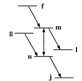
FIG. 1.: Term diagram.

We consider the photon emission of two monochromatic fields interacting with an atom whose term system is shown in Fig. 1. One of the two fields is regarded as strong and it resonates with the $m-n$ transition, the matrix element of interaction (traveling wave) is

$$V_{mn}\exp\{i\omega_{mn}t\}=-G\exp\{-i(\Omega t-kr)\}.$$ (2.1)

$$G=d_{mn}E/2\hbar,\quad\Omega=\omega_{\mu}-\omega_{mn}.$$ (2.2)

We are interested in emission or absorption of photons of a field resonating with one of the four transitions. $nj$, $m-l$, $fm$, and $gn$ (Fig.1). For example in the case of $nj$

$$V_{nj}\exp\{i\omega_{nj}t\}=-G_{\mu}\exp\{-i(\Omega_{\mu}t-k_{\mu}r)\},$$ (2.3)

$$G_{\mu}=d_{nj}E_{\mu}/2\hbar,\quad\Omega_{\mu}=\omega_{\mu}-\omega_{nj}$$ (2.4)

The system of equations for the density matrix has the form

$$L_{jj}\rho_{jj}=V_{nj}\rho_{nn}+q_{j},$$ (2.5)

$$L_{jn}\rho_{jn}=-iV_{mn}\exp\{i\omega_{mn}t\}\rho_{jm}=$$ (2.6)

$$=iV_{nj}^{*}\exp\{-i\omega_{nj}t\}(\rho_{nn}-\rho_{jj}),$$ (2.7)

$$L_{jm}\rho_{jm}=-iV_{mn}^{*}\exp\{-i\omega_{mn}t\}\rho_{jn}=$$ (2.8)

$$=-iV_{nj}^{*}\exp\{-i\omega_{nj}t\}\rho_{nm};$$ (2.9)

$$L_{mm}\rho_{mm}=+2Re[iV_{mn}\exp\{i\omega_{mn}t\}\rho_{nm}]=q_{m},$$ (2.10)

$$L_{nn}\rho_{nn}=-2Re[iV_{mn}\exp\{i\omega_{mn}t\}\rho_{nm}]=q_{n}+\gamma_{mn}\rho_{mm},$$ (2.11)

$$L_{nm}\rho_{nm}=iV_{nm}\exp\{-i\omega_{mn}t\}(\rho_{nn}-\rho_{mm})=q_{m},$$ (2.12)

$$L_{ik}=\partial/\partial\,t+v\nabla+\Gamma_{ik},\quad\Gamma_{ll}\equiv\Gamma_{l},$$ (2.13)

$\Gamma_{ik}$ are transition widths and $q_{i}$ is the rate of excitation of atoms to the state $i$, $\rm v$.

According to (2.9) and (2.13) the field $V_{jn}$ does not affect the population (”weak field”). Therefore the entire system of equations was found to be split up; eqs. (2.13) include only $\rho_{mm}$, $\rho_{nn}$, and $\rho_{nm}$, and the solution of the system serves as a ”source” for the computation of $\rho_{jm}$, $\rho_{jn}$ and $\rho_{jj}$ from (2.9). In the case of (2.1) and (2.3) the system (2.9) (2.13) reduces to equations whose solution has the form

$$\rho_{jj}=n_{j}+\dfrac{\gamma_{nj}}{\Gamma_{j}}\rho_{nn},$$ (2.14)

$$\rho_{nn}=n_{n}+\dfrac{2\pi G^{2}}{\Gamma_{n}\sqrt{1+\ae}}\left(1-\dfrac{\gamma_{mn}}{\Gamma_{n}}\right)(n_{m}-n_{n})W_{B}(v),$$ (2.15)

$$\rho_{mm}=n_{m}-\dfrac{2\pi G^{2}}{\Gamma_{m}\sqrt{1+\ae}}(n_{m}-n_{n})W_{B}(v),$$ (2.16)

$$\rho_{nm}=r_{nm}\exp\{-i(\Omega t-kr)\},$$ (2.17)

$$r_{nm}=iG(\rho_{mm}-\rho_{nn})/(\Gamma+i\Omega^{\prime})$$ (2.18)

where

$$W_{B}(v)=\Gamma_{B}/\pi[\Gamma_{B}^{2}+(\Omega-kv)^{2}],\ \Gamma_{B}=\Gamma\sqrt{1+\ae},$$ (2.19)

$$\Gamma\equiv\Gamma_{nm},\quad\Omega^{\prime}=\Omega-kv,$$ (2.20)

$${\Omega_{\mu}}^{\prime}=\Omega_{\mu}-k_{\mu}v,\ \ae=\tau^{2}G^{2}=\frac{2(\Gamma_{m}+\Gamma_{n}-\gamma_{mn})}{\Gamma_{m}\Gamma_{n}\Gamma},$$ (2.21)

$$n_{i}=\frac{q_{i}(v)}{\Gamma_{i}}+\frac{\gamma_{ki}}{\Gamma_{i}}\cdot\frac{q_{k}(v)}{\Gamma_{k}}$$ (2.22)

The quantities $n_{i}(v)$ represent velocity distributions of atoms in the absence of a strong field $(G=0)$ determined by excitation processes $q_{i}(v)$.

The emission (absorption) power is determined by the general formula

$$w_{nj}=-2\hbar\omega_{nj}Re\langle iV_{nj}\exp\{i\omega_{nj}t\}\rho_{jn},\rangle$$ (2.23)

where the angle brackets designate averaged velocities $v$ of atoms. Using the system (2.9) we can express $\rho_{jn}$ in terms of (2.18) and obtain an expression for power (2.23) in the form

$$w_{nj}=2\hbar\omega_{nj}|G_{\mu}|^{2}Re\left\langle\frac{[\Gamma_{jm}+i({\Omega_{\mu}}^{\prime}+\Omega^{\prime})](\rho_{nn}-\rho_{jj})-iGr_{nm}}{[\Gamma_{jm}+i({\Omega_{\mu}}^{\prime}+\Omega^{\prime})][\Gamma_{jn}+i{\Omega_{\mu}}^{\prime}]+G^{2}}\right\rangle.$$ (2.24)

Equation (2.24) clearly reflects the classification of effects due to the external field. The denominator contains squares $\Omega_{\mu}$ terms, i.e., it contains resonances at two frequencies. This can be interpreted as a splitting of the atom levels in the external field The numerator in (2.24) contains two terms with significantly different properties. The first term is proportional to the population difference $\rho_{nn}-\rho_{jj}$ containing Bennett’s ”holes,” as reflected in the factor $W_{B}(v)$ (henceforth called the Bennett distribution). The second term proportional to $r_{nm}$ varies only the the shape but not its integral intensity, since

$$\int\limits_{-\infty}^{+\infty}w_{nj}d\Omega_{\mu}=2\pi\hbar\omega_{nj}|G_{\mu}|^{2}<\rho_{nn}-\rho_{jj}>.$$

The fact that this term appeared and its property are not at all specific to the special case under consideration. According to (2.9) the ”sources” that ”excite” $\rho_{jm}$ and $\rho_{jn}$ are both the population difference $\rho_{nn}-\rho_{jj}$ and the non-diagonal element $\rho_{nm}$ stimulated by the strong field for any spectral composition of the strong field. Therefore $w_{nj}$ contains $\rho_{nm}$ also in the general case, and not only in a monochromatic field. We can say that this term reflects the ”coherence” that is contributed to the atomic state by the strong field, so that a weak field ”mixes” the m and j states as well as the n and j elates. The last circumstance causes oscillations at the frequency $\omega+\omega_{\mu}$. The above properties of the term with $r_{nm}$ allow us to call the associated phenomena nonlinear interference effects.

We can regard (2.24) as the difference between the number of acts of emission and absorption of the $\hbar\omega_{\mu}$ photon. All the terms of $w_{nj}$ except $\rho_{jj}$ determine emission processes. Conversely terms associated with $\rho_{jj}$ control the weak field energy absorption rate. According to (2.24) only the level splitting effect stands out in the absorption probability^[2,3,6,14]. This is due to the fact that absorption corresponds to the transition from the unexcited level $j$ to excited level $n$. NIE is due to the reverse transition from an excited to unexcited state, i.e., in the case when $n-j$ are contained only in the emission. Therefore the line shapes of pure emission and absorption turn out to be different due to NIE. The sign of their difference, i.e., of $w_{nj}$, is determined not only by the sign of population difference $\rho_{nn}-\rho_{jj}$; in particular the sign of $w_{nj}$ can change with the change of $\Omega_{\mu}$ ^[7-9].

Equation (2.24) makes it possible to analyze also spontaneous emission. For this purpose it is merely necessary to drop the term $\rho_{jj}$ from (2.24) and replace $|G_{\mu}|^{2}$ by a quantity corresponding to the atomic interaction with zero oscillations of the field^[15]: $\gamma_{nj}(8\pi^{2})^{-1}\Delta\Omega_{\mu}\Delta O$. Equations for other transitions are of the same type and can be obtained from (2.24) by a simple substitution of indices and signs. For example, $w_{ml}$ is obtained from the substitutions $m\rightarrow n$, $j\rightarrow l$, and $\Omega^{\prime}\rightarrow-\Omega^{\prime}$.

3 EMISSION AND ABSORPTION LINE SHAPE IN TRAVELING MONOCHROMATIC WAVE FIELD

We analyze the role of nonequilibrium velocity distribution and nonlinear interference effects. We consider first two directions of $k_{\mu}$ in detail: along and against k. The value of $w_{nj}$ averaged over $\rm v$ for these two directions is

$$w_{nj}^{\pm}=2\hbar\omega_{nj}|G_{\mu}|^{2}\frac{\sqrt{\pi}}{k{\bar{v}}}\exp\left\{-\frac{\Omega_{\mu}^{2}}{(k_{\mu}{\bar{v}})^{2}}\right\}\times$$ (3.1)

$$\times\{N_{n}-N_{j}+(N_{m}-N_{n})Re[F_{\pm}(\Omega_{\mu})+f_{\pm}(\Omega_{\mu})]\},$$ (3.2)

$$F_{\pm}+f_{\pm}=\frac{k_{\mu}}{k}\frac{2G^{2}}{\sqrt{1+\ae}}\times$$ (3.3)

$$\times\frac{\Gamma_{n}^{-1}(1-\gamma_{mn}/\Gamma_{m})[\Gamma_{\pm}+iz]+[1\pm\sqrt{1+\ae}]/2}{[\Gamma_{0}+iz][\Gamma_{\pm}+iz]+G^{2}},$$ (3.4)

$$z=\Omega_{\mu}\mp\Omega k_{\mu}/k,\Gamma_{0}=\Gamma_{jn}+\Gamma_{B}k_{\mu}/k,$$ (3.5)

$$\Gamma_{\pm}=\Gamma_{jm}+\Gamma_{B}(k_{\mu}/k\pm 1),\ \Gamma_{B}=\Gamma\sqrt{1+\ae}.$$ (3.6)

The signs + and - in (3.3) correspond to $k_{\mu}$ directed along and against k; $f_{\pm}$ and $F_{\pm}$ represent the interference term and a term due to the nonequilibrium addition to the velocity distribution, respectively. Equation (3.3) is not applicable if $k_{\mu}<k$ and ${\bf k}_{\mu}\cdot{\bf k}<0$. Velocity averaging can be performed also in this case. However the obtained expression can be used to some extent in the analysis only if $\ae$ is small Then (3.3) is valid if $\Gamma_{-}$ is replaced by $\Gamma_{jm}k_{\mu}/k+(1-k_{\mu}/k)\Gamma_{jn}$, $G=0$ and $\ae=0$ everywhere (except for the common factor $G^{2}$), and $[1+\sqrt{1+\ae}]/2$ is replaced by $k_{\mu}/k$.

A comparison of (3.3) with (2.24) shows that $w_{nj}$ has the same formal structure as the corresponding expression for the fixed atom whose resonant frequency is converted with respect to the Bennet distribution maximum and which has the widths $\Gamma_{\pm}$ and $\Gamma_{0}$ instead of $\Gamma_{jm}$ and $\Gamma_{jn}$ respectively. The physical meaning of $\Gamma_{0}$ and $\Gamma_{\pm}$ is as follows. The perturbation theory distinguishes between step-wise and two-photon processes whose line shape is determined by the factors $<[\Gamma_{jn}+i(\Omega_{\mu}-{\bf k}_{\mu}\cdot{\bf v})]^{-1}>$ and $<\{\Gamma_{jm}+i[(\Omega_{\mu}+\Omega)-({\bf k}_{\mu}+{\bf k})\cdot{\bf v}]\}^{-1}>$. In our case the averaging is carried out essentially with the Bennett distribution (since $\Gamma_{B}\ll k_{\mu}\bar{v}$) and the result of the averaging is $[\Gamma_{0}+iz]^{-1}$ and $[\Gamma_{\pm}+iz]^{-1}$^[16]. Consequently $\Gamma_{0}$ is the line width of a step-wise transition that is the sum of the width $\Gamma_{B}k_{\mu}/k$ of the velocity distribution converted with respect lo Doppler shifts in the $\omega_{nj}$ region and the natural width $\Gamma_{jn}$ of the $n-j$ transition. Correspondingly $\Gamma_{\pm}$ is the line width of two-photon transition consisting of the natural part $\Gamma_{jm}$ and the Doppler part $\Gamma_{B}(k_{\mu}/k\pm 1)$. Thus the physical meaning of the analogy between (3.3) and the line shape of an ”effective atom” is quite clear. The ”effective atom” represents the group of atoms that interact with a strong field. The ”effective atom” has the same system of terms as in Fig.1 except that the widths are changed in accordance with the Bennett distribution and frequency-correlated properties of the step-wise and two-photon processes^[16].

Just as in the case of an individual atom, the step- wise and two-photon processes in the ”effective atom” cannot be considered independently if $G$ is sufficiently large^[16]. In fact the numerator in (3.3) contains $G^{2}$ and its expansion in terms of simple fractions

$$\frac{1}{[\Gamma_{0}+iz][\Gamma_{\pm}+iz]+G^{2}}$$ (3.7)

$$=\frac{1}{(z_{1}+iz)(z_{2}+iz)}$$ (3.8)

$$=\frac{1}{z_{1}-z_{2}}\left[\frac{1}{z_{2}+iz}-\frac{1}{z_{1}+iz}\right].$$ (3.9)

$$z_{1,2}=1/2\{\Gamma_{0}+\Gamma_{\pm}\pm\sqrt{(\Gamma_{0}-\Gamma_{\pm})^{2}}-4G^{2}\}$$ (3.10)

yields resonant numerators with $z_{1},\>z_{2}$ rather than with $\Gamma_{0},\>\Gamma_{\pm}$. Under certain conditions the radical in (3.3) can turn out to be imaginary, which would correspond to the splitting of the levels of an effective atom.

Equation (3.3) shows that when $\gamma_{mn}=\Gamma_{m}$ the effect of velocity distribution variation is completely eliminated and only the NIE remains. The physical meaning of this is quite clear. The external field transfers some atoms from the upper level to the lower; at the same time however the relaxation transition is reduced by the same quantity since there are no other channels of decay from the upper level. On the other hand the polarization stimulated by the field at the transition $mn$ does not turn to zero (see (2.24), expression for $r_{nm}$ and NIE remains unchanged. The transition $6p^{1}P_{2}^{0}-7s^{3}S_{1}$ of mercury, $\lambda=1.529$, at which generation was observed^[7] can serve as an example of a case in which the condition $\gamma_{mn}=\Gamma_{m}$ is valid.

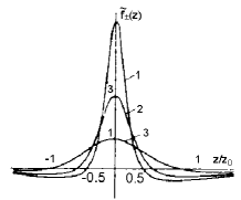
FIG. 2.: Plots of the frequency dependence of the function $\tilde{f}_{\pm}$ ($z=\Omega_{\mu}\mp\Omega k_{\mu}/k$) for real $z_{1}$ and $z_{2}$. The curves correspond to the following values: $1-z_{1}/z_{2}=5$; $2-z_{1}/z_{2}=2.5$; $3-z_{1}/z_{2}=1$.

The interference effect. We examine the interference term $f_{\pm}(\Omega_{\mu})$ in greater detail. Based on (3.3) and (3.10) we have

$$f_{\pm}(\Omega_{\mu})=\frac{k_{\mu}}{k}\frac{G^{2}}{\sqrt{1+\ae}}\frac{1\mp\sqrt{1+\ae}}{z_{1}-z_{2}}\left[\frac{1}{z_{2}+iz}-\frac{1}{z_{1}+iz}\right].$$ (3.11)

The line contour of $Re[f_{\pm}(\Omega_{\mu})]$ has the simplest shape when $z_{1,2}$ are real. In this case it follows from (3.11) that the function $Ref_{\pm}$ changes sign in going from the center of the line to the wings. The sign of $Ref_{+}$ at the point $z=0$ is determined by the factor $1+\sqrt{1+\ae}$ and depends therefore on the relative direction ${\bf k}_{\mu}$ and ${\bf k}$. When ${\bf k}_{\mu}\cdot{\bf k}>0$ the value in the center is negative and in the opposite direction it is positive. When the values of the external field are small ($\ae\lesssim 1$) we have $Ref_{+}\sim\ae^{2}$ and $Ref_{-}\sim\ae$.

The function

$$f_{\pm}(z)=\left[\frac{k_{\mu}}{k}\frac{G^{2}}{\sqrt{1+\ae}}\frac{1\mp\sqrt{1+\ae}}{z_{1}^{2}}\right]^{-1}Ref_{\pm}(z)$$

is illustrated in Fig.2 for $z_{1}/z_{2}=1;2.5;5$. According to Fig. 2 the graphs have an approximately similar shape (the positive maximum in the center and broad negative wings) for any values of $z_{1}/z_{2}$. However the larger $z_{1}/z_{2}$ the narrower and more intense the maximum. When $z_{2}\ll z_{1}$ its width is approximately equal to $z_{2}$ and its intensity in the center is proportional to $z_{2}^{-1}$. This case seems to be the most interesting from the practical point of view.

We consider the conditions for which the relation $z_{2}\ll z_{1}$ is valid. For the ”interference” direction ${\bf k}_{\mu}\cdot{\bf k}<0$, in which the effect is sharper, the expressions for $z_{1,2}$ can be represented in the form

$$z_{1,2}=\frac{1}{2}\left\{\Gamma_{jn}+\Gamma_{jm}+\Gamma_{B}\left(\frac{2k_{\mu}}{k}-1\right)\right.$$ (3.12)

$$\left.\pm\sqrt{(\Gamma_{B}+\Gamma_{jn}-\Gamma_{jm})^{2}-4G^{2}}\right\}.$$ (3.13)

According to this formula the absence of splitting and the considerable difference between $z_{1}$ and $z_{2}$, are due to the conditions

$$\Gamma+\Gamma_{jn}\gg\Gamma_{jm},\>k_{\mu}\approx k,\>\Gamma^{2}\ae/G^{2}=(\Gamma\tau)^{2}\gg 1.$$ (3.14)

Here the radical in (3.12) can be expanded into a series:

$$z_{1}=\Gamma_{jn}+\Gamma\frac{k_{\mu}}{k}\sqrt{1+\ae}-\frac{\ae/\tau^{2}}{\Gamma\sqrt{1+\ae}+\Gamma_{jn}-\Gamma_{jm}},$$ (3.15)

$$z_{2}=\Gamma_{jm}+\Gamma\left(\frac{k_{\mu}}{k}-1\right)\sqrt{1+\ae}+\frac{\ae/\tau^{2}}{\Gamma\sqrt{1+\ae}+\Gamma_{jn}-\Gamma_{jm}}.$$ (3.16)

We see from (3.15) that the minimum value of $z_{2}$ equals the line width of the forbidden transition $\Gamma_{jm}$. In many cases we can expect that $\Gamma_{jm}\ll\Gamma{jn}$. Consequently the emission spectrum at the transition $j-n$ can contain a structure with a considerably smaller width than is typical of the given transition. The value of $z_{2}$ increases with the field but much slower than $z_{1}$ when $(k_{\mu}-k)/k\ll 1$.

The amplitude of the interference term

$$f_{-}(0)=\frac{k_{\mu}}{k}\frac{1+\sqrt{1+\ae}}{\sqrt{1+\ae}}\frac{G^{2}}{z_{1}z_{2}}=\frac{k_{\mu}}{k}\frac{1+\sqrt{1+\ae}}{\sqrt{1+\ae}}\frac{G^{2}}{\Gamma_{0}\Gamma_{-}+G^{2}}$$ (3.17)

as a function of $G^{2}$ is a curve with saturation where one half of the maximum value is reached approximately for $G^{2}=\Gamma_{0}\Gamma_{-}$. Therefore the ratio $G^{2}/\Gamma_{0}\Gamma_{-}\equiv\ae_{-}$ can be interpreted as the saturation parameter of the effective atom. If $(k_{\mu}-k)/k\ll 1$ and $\Gamma_{0}\gg\Gamma_{-}$, the width $z_{2}\approx\Gamma_{jm}[1+\ae_{-}]$ is also determined by the quantity $\ae_{-}$. We note that $\ae_{-}<\ae$. In tact, according to (3.14) and (2.22)

$$\frac{\ae}{\ae_{-}}=\Gamma_{0}\Gamma_{-}\tau^{2}=2\left[\Gamma_{jm}+\left(\frac{k_{\mu}}{k}-1\right)\Gamma\sqrt{1+\ae}\right]\times$$ (3.18)

$$\left[\Gamma_{jn}+\frac{k_{\mu}}{k}\Gamma\sqrt{1+\ae}\right]\frac{\Gamma_{m}+\Gamma_{n}-\gamma_{mn}}{\Gamma_{m}\Gamma\Gamma_{n}}.$$ (3.19)

By virtue of the obvious inequalities $2\Gamma_{-}>\Gamma_{m}$, $\Gamma_{0}>\Gamma$ and $\Gamma_{m}+\Gamma_{n}-\gamma_{mn}>\Gamma_{n}$, the right-hand side in (3.19) is larger than unity. Therefore as $G^{2}$ increases the population difference in the center of the Bennett distribution is equalized first since it is proportional to $\ae/(1+\ae)$. The amplitude of the interference term is determined by the ratio $\ae_{-}/(1+\ae_{-})$, retains its linear dependence up to large values of $G^{2}$, and becomes saturated at $\ae_{-}\approx 1$. At the same time the width of the central maximum increases, becoming twice as large at $\ae_{-}=1$ at the same value of the field.

We now consider the behavior of the interference term when ${\bf k}_{\mu}$ is parallel to ${\bf k}$. We first show that $z_{1}$ and $z_{2}$ cannot differ significantly in this case. In fact, it follows from (3.10) that $z_{1}$ and $z_{2}$ differ sharply if $\Gamma_{0}+\Gamma_{+}$$\approx\Gamma_{0}-\Gamma_{+}$ or $\Gamma_{0}+\Gamma_{+}$$\approx\Gamma_{+}-\Gamma_{0}$. These conditions in turn are equivalent to the inequality systems (see (3.5)) $\Gamma_{jm}\gg\Gamma$, $\Gamma_{jm}\gg\Gamma_{jn}$ or $\Gamma_{jn}\gg\Gamma$, $\Gamma_{jn}\gg\Gamma_{jm}$ which can be readily shown to be invalid in spontaneous relaxation and in impact broadening of lines. Consequently the roots $z_{1}$ and $z_{2}$ are of the same order of magnitude in the direction ${\bf k}_{\mu}\cdot{\bf k}>0$ and the structure is relatively not sharp. According to (3.11) the amplitude $f_{+}(0)$ is

$$f_{+}(0)=-\frac{k_{\mu}}{k}\frac{\sqrt{1+\ae}-1}{\sqrt{1+\ae}}\frac{G^{2}}{\Gamma_{0}\Gamma_{+}+G^{2}}.$$ (3.20)

Comparing (3.20) and (3.17) we see that $|f_{+}(0)|<f_{-}(0)$, i.e., the amplitude of the structure in the direction ${\bf k}_{\mu}\cdot{\bf k}>0$ is always smaller than for ${\bf k}_{\mu}\cdot{\bf k}<0$.

So far we considered $z_{1},\>z_{2}$ to be real. Now let

$$z_{1,2}=z_{0}+i\zeta,z_{0}=(\Gamma_{0}+\Gamma_{\pm})/2,$$ (3.21)

$$\zeta=\sqrt{G^{2}-(\Gamma_{0}-\Gamma_{\pm})^{2}/4},$$ (3.22)

$$Ref_{\pm}(z)=\frac{k_{\mu}}{k}\frac{1\mp\sqrt{1+\ae}}{\sqrt{1+\ae}}\frac{G^{2}}{2\zeta}\times$$ (3.23)

$$\times\left[\frac{z+\zeta}{z_{0}^{2}+(z+\zeta)^{2}}-\frac{z-\zeta}{z_{0}^{2}+(z-\zeta)^{2}}\right].$$ (3.24)

The general shape of the graph $Ref_{\pm}$ depends on the ratio $\zeta/z_{0}$, as is apparent from Fig.5. When $\zeta/z_{0}$ is small the contours are qualitatively indistinguishable from the case of real, but similar, $z_{1},\>z_{2}$ (see curves 1 and 2 in Fig.5). It is of interest therefore to determine the maximum possible values for the ratio $\zeta/z_{0}$S. We can show using (3.21) and (3.3) that under the most favorable conditions $\zeta\leq\sqrt{3}z_{0}$. The curve in Fig.5 corresponding to $\zeta=\sqrt{3}z_{0}$ indicates the maximum effect of line splitting. The ”fuzzy” splitting of the interference term has a physical meaning: the increasing $G^{2}$ is accompanied by a rise in the atomic level splitting occurring together, however, with an increase in the line widths of effective atom, $\Gamma_{0}$, and $\Gamma_{\pm}$ due to the broadening of Bennett distribution (see (2.22)). Nevertheless we can observe level splitting even with a large Doppler broadening since the shape of curve 3 in Fig.5 is still significantly different from the others.

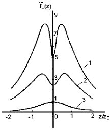
FIG. 3.: Plots of the frequency dependence of the function $\tilde{f}_{\pm}$ for complex $z_{1}$ and $z_{2}$ ($z_{1,2}=z_{0}\pm i\zeta$). The curves correspond to the following values: $1-\zeta=0$; $2-\zeta=z_{0}$; $3-\zeta=\sqrt{3}z_{0}$.

FIG. 4.: Plots of the frequency dependence of the function $\tilde{f}_{\pm}$ for real $z_{1}$ and $z_{2}$. The curves correspond to the following values: $1-z_{1}/z_{2}=5$; $2-z_{1}/z_{2}=2.5$; $3-z_{1}/z_{2}=1$.

FIG. 5.: Plots of the frequency dependence of the function $\tilde{f}_{\pm}$ for complex $z_{1}$ and $z_{2}$, $\zeta=z_{0}$. The curves correspond to the following values: $1-c=-1$; $2-c=0$; $3-c=1$

Nonequilibrium addition to the velocity distribution. We turn to the term $F_{\pm}(\Omega_{\mu})$ in (3.3):

$$F_{\pm}(\Omega_{\mu})=\frac{k_{\mu}}{k}\Gamma_{n}^{-1}\left(1-\frac{\gamma_{mn}}{\Gamma_{m}}\right)\frac{G^{2}}{\Gamma_{n}\sqrt{1+\ae}}\frac{1}{z_{1}-z_{2}}\times$$ (3.25)

$$\times\left[\frac{z_{1}-\Gamma_{\pm}}{z_{1}+iz}-\frac{z_{2}-\Gamma_{\pm}}{z_{2}+iz}\right].$$ (3.26)

In the case of real $z_{1,2}$ the sign of $z_{1}-\Gamma_{\pm}$ and $z_{2}-\Gamma_{\pm}$ is the same but depends on the sign of $\Gamma_{0}-\Gamma_{\pm}$. If $\Gamma_{0}>\Gamma_{\pm}$ then $z_{1,2}-\Gamma_{\pm}>0$; on the other hand, if $\Gamma_{0}<\Gamma_{\pm}$ then $z_{1,2}-\Gamma_{\pm}<0$ (see (3.10)). According to Fig.5 of particular interest is the case of strongly different $z_{1}$ and $z_{2}$ when $Re[F_{\pm}(z)]$ has the form of a broad dispersive contour (the width $z_{1}$) with a sharp notch (or spike) in the center (the width of $z_{2}\ll z_{1}$). The conditions that allow for $z_{1}\gg z_{2}$ were analyzed above. We note that $z_{2}\ll z_{1}$ can be realized when ${\bf k}_{\mu}\cdot{\bf k}<0$.

If $z_{1,2}$ are complex, $Re[F_{\pm}(\Omega_{\mu})]$ has the form

$$Re[F_{\pm}(\Omega_{\mu})]=\frac{k_{\mu}}{k}\frac{z_{0}}{\Gamma_{n}}\left(1-\frac{\gamma_{mn}}{\Gamma_{m}}\right)\frac{G^{2}}{\sqrt{1+\ae}}\left\{\frac{1}{z_{0}^{2}+(z+\zeta)^{2}}\right.$$ (3.27)

$$\left.+\frac{1}{z_{0}^{2}+(z-\zeta)^{2}}-\frac{\Gamma_{0}-\Gamma_{\pm}}{\Gamma_{0}+\Gamma_{\pm}}\frac{1}{\zeta}\left[\frac{z+\zeta}{z_{0}^{2}+(z+\zeta)^{2}}-\frac{z-\zeta}{z_{0}^{2}+(z-\zeta)^{2}}\right]\right\}.$$ (3.28)

In contrast to (3.23) the possibility to observe splitting is determined now not only by the ratio $\zeta/z_{0}$ but also by the magnitude and sign of the factor $(\Gamma_{0}-\Gamma_{\pm})/(\Gamma_{0}+\Gamma_{\pm})$. From (3.5) for $\Gamma_{0},\>\Gamma_{\pm}$ we can see that $-1<s\equiv(\Gamma_{0}-\Gamma_{\pm})/(\Gamma_{0}+\Gamma_{\pm})<1$. Figure 5 shows plots of

$$F_{\pm}=\left[\frac{k_{\mu}}{k}\left(1-\frac{\gamma_{mn}}{\Gamma_{m}}\right)\frac{G^{2}}{z_{0}\Gamma_{n}\sqrt{1+\ae}}\right]ReF_{\pm}$$

for the limiting values of the factor $s$ and for $\Gamma_{0}=\Gamma_{\pm}$. According to Fig.5, a sharply defined splitting effect can occur even with $\zeta=z_{0}$ which is less than the possible limit of $\zeta\leq z_{0}\sqrt{3}$. Particularly significant is curve 3 in Fig.5 according to which the intensity is much lower in the center than in the side maxima. Using (3.28) we can obtain for $\zeta=z_{0}$, ${\bf k}_{\mu}\cdot{\bf k}<0$ and $k_{\mu}=k$:

$$\frac{Re[F_{-}(0)]}{Re[F_{-}(\zeta)]}=\frac{5}{2}\frac{\Gamma_{-}}{\Gamma_{0}+2\Gamma_{-}}\approx\frac{5}{2}\frac{\Gamma_{jm}}{\Gamma_{jn}+2\Gamma_{jm}+\Gamma\sqrt{1+\ae}}.$$ (3.29)

Consequently if $\Gamma_{jn}+\Gamma_{B}\gg\Gamma_{jm}$, the ratio (3.29) is much smaller than unity. The condition $\Gamma_{0}\gg\Gamma_{-}$ corresponds to the value $s=1$ and it can be satisfied for $\Gamma\sqrt{1+\ae}\gg\Gamma_{jm}$.

Comparison of $F_{\pm}(\Omega_{\mu})$ and $f_{\pm}(\Omega_{\mu})$. It is clear from the preceding discussion that the frequency dependences of $F_{\pm}$ and $f_{\pm}$ are similar in general and in some cases one term can emphasize or, conversely, concentrate the effects contributed by the other.

We now consider the properties of the sum $F_{\pm}$ and $f_{\pm}$ and determine the weight of each of the two terms. We begin with the case of real roots $z_{1,2}$. In this case the curves $Re[F_{\pm}(z)]$ and $Re[f_{\pm}(z)]$ are of the same type throughout and we may limit the analysis to a single point $z=0$ (maximum or minimum). From (3.5) and (3.10) we find

$$Re[F_{\pm}(0)+f_{\pm}(0)]=\frac{k_{\mu}}{k}\frac{G^{2}\Gamma_{\pm}}{z_{1}z_{2}\sqrt{1+\ae}}\left[\frac{2}{\Gamma_{n}}\left(1-\frac{\gamma_{mn}}{\Gamma_{m}}\right)+\right.$$ (3.30)

$$\left.+\frac{1}{\Gamma_{\pm}}(1\mp\sqrt{1+\ae})\right].$$ (3.31)

The first term in the brackets is associated with $f_{\pm}$ and the second with $f_{\pm}$. The appearance of the factors $1/\Gamma_{n}$ and $1/\Gamma_{\pm}$ is understandable: $1/\Gamma_{n}$ determines the time of interaction of an atom at the n level with the field. An analog of such an ”accumulation time” for the interference term is the quantity $1/\Gamma_{\pm}$.

In addition to the factor $1-\gamma_{mn}/\Gamma_{m}$, whose role was discussed above, the relation between $F_{\pm}(0)$ and $f_{\pm}(0)$ depends on the relaxation constants, field amplitude, direction of observation, and the ratio $k_{\mu}/k$. To observe NIE even with $\gamma_{mn}\ll\Gamma_{m}$ the most convenient conditions obtain when $k_{\mu}=-k$ and $\Gamma_{jm}\ll\Gamma_{n}$; furthermore its role increases with the rise in field intensity. Conversely when $\bf k$ and ${\bf k}_{\mu}$ are parallel we can expect an almost complete elimination of NIE because the inequality $\Gamma_{+}\gg\Gamma_{n}[\sqrt{1+\ae}-1]/2$ can be assured by $\Gamma_{jm}\gg\Gamma_{n}$, $\Gamma\gg\Gamma_{n}$, $\ae\ll 1$ and $k_{\mu}>k$. Therefore $Re[F_{\pm}]$ as well as $Re[f_{\pm}]$ can be predominant depending on the values of the numerous variable parameters.

If $z_{1,2}$ are complex the expression for $Re[F_{\pm}+f_{\pm}]$ differs from (3.28) only by the substitution of factor $s$

$$c=\frac{\Gamma_{0}-\Gamma_{\pm}}{\Gamma_{0}+\Gamma_{\pm}}-\frac{\Gamma_{n}}{\Gamma_{0}+\Gamma_{\pm}}\left(1-\frac{\gamma_{mn}}{\Gamma_{m}}\right)^{-1}[1\mp\sqrt{1+\ae}],$$ (3.32)

where the second term reflects the role of $Re[f_{\pm}]$. We can show that the value of $c$ varies between +1 and -1 Therefore the total contour can be deformed within the same limits as $Re[F_{\pm}]$ (see Fig.5).

We now consider $w_{nj}$ for the intermediate values of the angle $\theta$ between $\bf k$ and ${\bf k}_{\mu}$. We denote the velocity component perpendicular to $\bf k$ by $\bf u$:

$$\Omega_{\mu}^{\prime}=\Omega_{\mu}-{\bf ku}\sin\theta-{\bf k}_{\mu}{\bf v}\cos\theta,\>\Omega^{\prime}=\Omega-{\bf kv}.$$ (3.33)

According to (3.33) the averaging with respect to $v$ leads as before to (3.5), except that ${\bf k}_{\mu}$ must be replaced by $k_{\mu}\cos\theta$ (apart from the common factor in $F_{\pm}$ and $f_{\pm}$) and $\Omega_{\mu}$ by $\Omega_{\mu}-ku\sin\theta$. The subsequent averaging with respect to $u$ can be carried out although only its result is given here When the angles are small, $\theta\ll\Gamma_{+}/k\bar{v}$, $\Gamma_{0}/k\bar{v}$, there is practically no variation of $w_{nj}$.

The same consideration applies to the angles $|\pi-\theta|\ll\Gamma_{-}/k{\bar{v}}$, $\Gamma_{0}/k{\bar{v}}$. When $|\theta|$ (or $|\pi-\theta|$) increases above the indicated values the spectral width of the functions $F_{\pm},\>f_{\pm}$ increases approximately as $k\bar{v}\sin\theta$ and reaches the full Doppler width when $\theta\approx\pi/2$. Since the integrated intensity of the correction to $w_{nj}$ due to strong field does not depend on $\theta$, the amplitude of this correction is $k\bar{v}/\Gamma_{0}$ times lower than in the above cases. All these phenomena are due to the fact that the strong field represents a plane monochromatic wave and causes changes in the distribution of only one velocity component Therefore the case of $\theta=0$ and the adjacent directions of $k_{\mu}$ is the most interesting one.

Our analysis deals with the case where both fields represent plane traveling waves. The experimenter may find it convenient to use a strong field within the resonator of a suitable gas laser^[4,11,12]. The strong field then has the form of a standing wave and the pattern of events is somewhat different. When the departure from resonance in the strong field is greater than the width of Bennett distribution ($|\Omega|>\Gamma_{0},\>\Gamma_{\pm}$), one can regard the two traveling waves as fully independent because they interact with different groups of atoms. Therefore the expression for $w_{nj}$ now contains, instead of $F_{+}(\Omega_{\mu})+f_{+}(\Omega_{\mu})$ or $F_{-}(\Omega_{\mu})+f_{-}(\Omega_{\mu})$, the sum of these terms

$$F_{+}(\Omega_{\mu})+f_{+}(\Omega_{\mu})+F_{-}(\Omega_{\mu})+f_{-}(\Omega_{\mu}).$$ (3.34)

All the singularities of the terms with indices + or - are now at the distance $\pm\Omega k_{\mu}/k$ from the line center (see definition of $z$ in (3.5)) and they overlap. Thus all that we said for the case of a strong field in the form of a traveling wave remains valid for that of a standing wave. At the same time different frequencies should produce effects corresponding to ”interference” and ”non-interference” directions.

On the other hand if the condition $|\Omega|>\Gamma$ does not hold, the Bennett distributions stemming from two opposed waves overlap and we have a different situation. We can say that the additive property of nonlinear effects due to opposed waves appears a priori in the first approximation (with respect to $G^{2}$), i.e., (3.34) is valid if $G^{2}$ is left in the expression for $F_{\pm}+f_{\pm}$ only in the form of a common factor. The invariance of (3.3) in successive approximations with respect to $G^{2}$’ is due to the fact that large fields generate a spatial inhomogeneity of the medium (with a period of $\lambda/2$)^[13]. Consequently the atomic probability amplitudes are subject to a form of phase modulation and the atomic levels are split into a number of sublevels larger than the two sublevels typical of the traveling wave. The above modulation was Investigated in ^[15,18] in the case of resonance fluorescence and it was found that the emission spectrum changed significantly.

4 GENERATION IN THE PRESENCE OF EXTERNAL FIELD

In Secs. 2 and 3 the fields that resonated with transitions $n-j$, $g-n$, etc., were considered weak (Fig.1). Experiments^[13] showed that generation at these transitions was a convenient method of studying NIE. Therefore we now consider generation at the $g-n$ transition (since it was studied in^[13]) The unsaturated (with respect to $G_{\mu}$) gain at the $g-n$ transition changes in an external field $G$ that is resonant with $m-n$ (see Sec. 3). To compute the generation power at $g-n$ we must know the saturation function of the $g-n$ transition We can show that once the conditions

$$|N_{m}-N_{n}|\frac{G^{2}}{\Gamma^{2}}\ll|N_{g}-N_{n}|,|N_{m}-N_{n}|\frac{G^{4}}{\Gamma^{4}}\ll|N_{g}-N_{n}|\frac{G_{\mu}^{2}}{\Gamma^{2}}$$ (4.1)

are satisfied, saturation at the $g-n$ transition is the same as in the case of $G=0$. Therefore the generation power is determined by the standard formula

$$\frac{\Gamma_{n}+\Gamma_{g}-\gamma_{ng}}{\Gamma_{n}\Gamma_{g}\Gamma_{ng}}G_{\mu}^{2}=\left[1-\frac{\Delta N\exp\{\Omega_{\mu}^{2}/(k_{\mu}{\bar{v}})^{2}\}+\alpha}{N_{g}-N_{n}}\right]\times$$ (4.2)

$$\times\left[1+\frac{\Gamma_{ng}^{2}}{\Gamma_{ng}^{2}+\Omega_{\mu}^{2}}\right]^{-1};$$ (4.3)

$$\alpha=\frac{k_{\mu}}{k}(N_{m}-N_{n})G^{2}\left\{\frac{1-\gamma_{mn}/\Gamma_{m}}{\Gamma_{n}\Gamma_{0}}\left[\frac{\Gamma_{0}^{2}}{\Gamma_{0}^{2}+(\Omega_{\mu}+k_{\mu}\Omega/k)^{2}}\right.\right.$$ (4.4)

$$\left.+\frac{\Gamma_{0}^{2}}{\Gamma_{0}^{2}+(\Omega_{\mu}-k_{\mu}\Omega/k)^{2}}\right]+\frac{1}{\Gamma+\Gamma_{gn}-\Gamma_{gm}}\times$$ (4.5)

$$\times\left.\left[\frac{\Gamma_{+}}{\Gamma_{+}^{2}+(\Omega_{\mu}-k_{\mu}\Omega/k)^{2}}-\frac{\Gamma_{0}}{\Gamma_{0}^{2}+(\Omega_{\mu}-k_{\mu}\Omega/k)^{2}}\right]\right\},$$ (4.6)

$$\Gamma_{0}=\Gamma_{gn}+\frac{k_{\mu}}{k}\Gamma,\Gamma_{+}=\begin{cases}\Gamma_{gm}k_{\mu}/k+(1-k_{\mu}/k)\Gamma_{gn},&k_{\mu}<k\\ \Gamma_{gm}+(k_{\mu}/k-1)\Gamma,&k_{\mu}>k\end{cases}$$ (4.7)

where $\Delta N$ is the threshold population difference for $G=0$ and $\Omega_{\mu}=0$. In the absence of the external field (4.2) determines the usual dependence of power on $\Omega_{\mu}$ with the ”Lamb dip”. The term $\alpha$ introduces an additional spectral structure.

We consider the case when the role of atomic collisions is small, so that $\Gamma+\Gamma_{gn}-\Gamma_{gm}=\Gamma_{n}$. A ”spike” or a ”dip” (depending on the sign of $N_{m}-N_{n}$) then appears at the frequency $\Omega_{\mu}=-\Omega k_{\mu}/k$

$$I_{-}=\frac{N_{m}-N_{n}}{N_{n}-N_{g}}\frac{k_{\mu}}{k}\frac{|G|^{2}}{\Gamma_{n}\Gamma_{0}}\left(1-\frac{\gamma_{mn}}{\Gamma_{m}}\right)\frac{\Gamma_{0}^{2}}{\Gamma_{0}^{2}+(\Omega_{\mu}+k_{\mu}\Omega/k)^{2}}.$$ (4.8)

Another ”spike” or ”dip” appears at $\Omega_{\mu}=k_{\mu}\Omega/k$ (Fig.6).

$$I_{+}=\frac{N_{m}-N_{n}}{N_{n}-N_{g}}\frac{k_{\mu}}{k}\frac{|G|^{2}}{\Gamma_{n}\Gamma_{0}}\left[\frac{\Gamma_{0}}{\Gamma_{+}}\frac{\Gamma_{+}^{2}}{\Gamma_{+}^{2}+(\Omega_{\mu}-k_{\mu}\Omega/k)^{2}}\right.-$$ (4.9)

$$\left.-\frac{\gamma_{mn}}{\Gamma_{m}}\frac{\Gamma_{0}^{2}}{\Gamma_{0}^{2}+(\Omega_{\mu}-k_{\mu}\Omega/k)^{2}}\right];$$ (4.10)

if $\Gamma_{m},\>\Gamma_{g}\ll\Gamma_{n}$ and $|1-k_{\mu}/k|\ll 1$ then $\Gamma_{+}\ll\Gamma$ and $\Gamma_{+}\ll\Gamma_{gn}$ (see (refe4.4)). Consequently we see from (4.8) and (4.9) that in this case the ”spikes” $I_{-}$ and $I_{+}$ differ sharply from each other in width and height. The second term in (4.9) contributes significantly only to the wings of the $I_{+}$, contour so that the width of this ”spike” is much smaller than the natural width at the $g-n$ transition. When $\gamma_{mn}=\Gamma_{m}$ the ”spike” $I_{-}$ vanishes and only the interference ”spike” $I_{+}$, remains with singularities in the wings (a ”spike” in a ”trough”). In the other limiting case of $\Gamma_{m}\gg\Gamma_{n},\>\Gamma_{g}$; $\Gamma_{+}\approx\Gamma_{0}$ both spikes have the same width and vanish when $\gamma_{mn}/\Gamma_{m}\rightarrow 1$. When $\Omega=0$ and $\Gamma_{+}\ll\Gamma_{gn}$, the above singularities occur in the floor of the Lamb ”dip” as shown schematically in Fig.6.

FIG. 6.: Frequency dependence of generation power

Two generation peaks differing in width were observed in^[13]. A strong frequency dependence of generation in the region $I_{+}$ can be utilized for effective output power stabilization of generation frequency.

We consider the dependence of generating emission frequency on the natural resonator frequency The generation frequency is determined by the requirement that the field phase shift in a double pass of the resonator be a multiple of $2\pi$. The value of the refraction index necessary to compute the phase can be found from

$$n_{0}=1+2\pi NRe\{r_{ng}d_{ng}\}(E_{\mu}/4)^{-1},$$

where $E_{\mu}$ is intensity of the field resonating with the $n-g$ transition. If $|\Omega_{\mu}|\ll k_{\mu}{\bar{v}}$ the generation frequency is determined from the equation

$$\Omega_{r}\equiv\omega_{r}-\omega_{gn}=\Omega_{\mu}+\frac{l}{l_{r}}\frac{\Delta\omega_{r}}{2}\times\left\{\frac{2}{\sqrt{\pi}}\frac{N_{g}-N_{n}}{\Delta N}\frac{\Omega_{\mu}}{k{\bar{v}}}\right.$$ (4.11)

$$\left.-\left[\frac{N_{g}-N_{n}}{\Delta N}-1\right]\frac{\Omega_{\mu}\Gamma_{ng}}{2\Gamma_{ng}^{2}-\Omega_{\mu}^{2}}-\frac{k_{\mu}}{k}|G|^{2}\frac{N_{m}-N_{n}}{\Delta N}\Phi(\Omega_{\mu})\right\},$$ (4.12)

where $\omega_{r}$ is the natural frequency of the resonator and

$$\Phi(\Omega_{\mu})=\left(1-\frac{\gamma_{mn}}{\Gamma_{m}}\right)\frac{1}{\Gamma_{n}}\left[\left(\Omega_{\mu}+\frac{k_{\mu}}{k}\Omega-\frac{\Gamma_{0}\Gamma_{ng}\Omega_{\mu}}{2\Gamma_{ng}^{2}+\Omega_{\mu}^{2}}\right)\times\right.$$

$$\times\frac{1}{\Gamma_{0}^{2}+(\Omega_{\mu}+k_{\mu}\Omega/k)^{2}}+$$

$$\left.+\left(\Omega_{\mu}-\frac{k_{\mu}}{k}\Omega-\frac{\Gamma_{0}\Gamma_{ng}\Omega_{\mu}}{2\Gamma_{ng}^{2}+\Omega_{\mu}^{2}}\right)\frac{1}{\Gamma_{0}^{2}+(\Omega_{\mu}-k_{\mu}\Omega/k)^{2}}\right]$$

$$+\frac{1}{\Gamma+\Gamma_{gn}-\Gamma_{gm}}\left[\left(\Omega_{\mu}-\frac{k_{\mu}}{k}\Omega-\frac{\Gamma_{+}\Gamma_{gn}\Omega_{\mu}}{2\Gamma_{ng}^{2}+\Omega_{\mu}^{2}}\right)\times\right.$$

$$\times\frac{1}{\Gamma_{+}^{2}+(\Omega_{\mu}-k_{\mu}\Omega/k)^{2}}-$$

$$\left.-\left(\Omega_{\mu}-\frac{k_{\mu}}{k}\Omega-\frac{\Gamma_{0}\Gamma_{gn}\Omega_{\mu}}{2\Gamma_{gn}^{2}+\Omega_{\mu}^{2}}\right)\frac{1}{\Gamma_{0}^{2}+(\Omega_{\mu}-k_{\mu}\Omega/k)^{2}}\right].$$

The first term in the curved brackets of (4.11) describes the known phenomenon of ”pulling” the generation frequency by the natural resonator frequency towards the center of the atomic line. The second describes a ”repulsion” of the generation frequency from the transition frequency towards the resonator frequency proportional to the quantity $(N_{g}-N_{n})/\Delta N-1$. On the curve of $\Omega_{\mu}$ as a function of $\Omega_{r}$ (Fig.7) the first effect corresponds to the deviation of the $\Omega_{\mu}$ asymptote from the straight line $\omega_{r}-\omega_{gn}=\Omega_{\mu}$ by an angle of the order of $\Delta\omega_{r}/k_{\mu}{\bar{v}}$, and the second effect corresponds to the singularity of the order of $\sqrt{2}\Gamma_{gn}$ near $\Omega_{\mu}=0$.

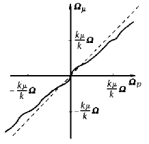
FIG. 7.: Generation frequency as a function of resonator frequency.

We consider singularities occurring in the curve $\Omega_{\mu}$ in the region of frequencies $|\Omega_{\mu}\pm\Omega k_{\mu}/k|\lesssim\Gamma_{+,0}$ if $\Gamma_{ng}\ll\Omega\ll k_{\mu}{\bar{v}}$. For a purely spontaneous relaxation and $\gamma_{mn}\ll\Gamma_{m}$ we obtain from (4.11)

$$\Omega_{r^{\pm}}=\Omega_{\mu}-\frac{l_{r}}{l}\frac{\Delta\omega_{r}}{2}\frac{N_{m}-N_{n}}{\Delta N}\frac{k_{\mu}}{k}\frac{|G|^{2}}{\Gamma_{n}\Gamma_{+,0}}\frac{\Gamma_{+,0}(\Omega_{\mu}\mp\Omega k_{\mu}/k)}{\Gamma_{+,0}^{2}+(\Omega_{\mu}\mp\Omega k_{\mu}/k)^{2}}.$$ (4.13)

The term proportional to $\Delta\omega_{r}/k_{\mu}{\bar{v}}$ has been dropped. It appears from (4.13) that in the presence of an external field when $\Omega_{\mu}=\pm\Omega k_{\mu}/k$ the dependence of generation frequency on the natural resonator frequency increases when $N_{m}-N_{n}>0$ and decreases when $N_{m}-N_{n}<0$:

$$\left(\frac{d\Omega_{\mu}}{d\Omega_{\mu}^{\pm}}\right)_{\Omega_{\mu}=\pm k_{\mu}\Omega/k}=\left[1-\frac{\Delta\omega_{r}}{2\Gamma_{\pm}}\frac{l}{l_{r}}\frac{N_{m}-N_{n}}{\Delta N}\frac{k_{\mu}}{k}\frac{G^{2}}{\Gamma_{n}\Gamma_{+,0}}\right].$$

In the latter case this phenomenon can be used for passive stabilization of the generation frequency. The lower the resonator $Q$ the greater this effect. If $\gamma_{mn}=\Gamma_{m}$ the singularity at $\Omega_{\mu}=-\Omega k_{\mu}/k$ vanishes. At $\Omega=0$ all the singularities in $\Omega_{\mu}$ as a function of $\Omega_{r}$ appear only when $|\Omega_{\mu}|\lesssim\max\{\Gamma_{ng},\Gamma_{0},\Gamma_{+}\}$. The dependence of $\Omega_{\mu}$ on $\Omega_{r}$ can be cumbersome in this case. However if $\Gamma_{+}\ll\Gamma_{ng},\Gamma_{0}$ the most pronounced is only the contribution from $\Gamma_{+}$.

Translated by S. Kassel 97

REFERENCES

[1]V. R. Bennett, Appl. Optics Suppl. No.1 on Optical
Masers, 1962, p.24.
[2]N. N. Kostin, V. A. Khodovoi, and V. V. Khromov,
Report to the IV Symposium on Nonlinear Optics, Kiev,
1968.
[3]Yu. M. Kirin, D. P. Kovalev, S. G. Rautian, and
R. I. Sokolovskii, ZhETF Pis. Red. 9, 7 (1969) [JETP
Lett. 9, 3 (1969)].
[4]M. S. Feld and A. Javan, Phys. Rev. Lett. 20, 578
(1968).
[5]S. G. Rautian, Proc. Symp. on Modern Optics, Polytechnic Press,1967, p.353.
[6]G. E. Notkin, S. G. Rautian, and A. A. Feoktistov,
Zh. Eksp. Teor. Fiz. 52, 1673 (1967) [Sov. Phys. JETP
25, 1112 (1967)].
[7]T. Ya, Popova and A. K. Popov, ibid. 52, 1517 (1967)
[25, 1007 (1967)].
[8]A. Javan, Phys. Rev. 107, 1579 (1957).
[9]S. G. Rautian and I. I. Sobel’man, Zh. Eksp. Teor.
Fiz. 41, 456 (1961) [Sov. Phys. JETP 14, 328 (1962)].
[10]H. K. Holt, Phys. Rev. Lett. 19, 1275 (1967).
[11]H. K. Holt, Phys. Rev. Lett. 20, 410 (1968).
[12]W. G. Schweitzer, Jr., M. M. Birky, and J. A. White,
J. Opt. Soc. Amer. 57, 1226 (1967).
[13]I. M. Beterov and V. P. Chebotaer, ZhETF Pis.
Red. 9, 216 (1969) [JETP Lett. 9, 127 (1969)].
[14]T. Jajima and K. Shimoda, Adv. Quant. Electr.,
Columbia Univ. Press, N. Y., London, 1961, p.548.
[15]S. G. Rautian and I. I. Sobel’man, Zh. Eksp. Teor.
Fiz. 44, 934 (1963) [Sov. Phys. JETP 17, 635 (1963)].
[16]T. Ya. Popova, A. K. Popov, S G. Rautian, and A. A.
Feoktistov, Zh. Eksp. Teor. Fiz. 57, 444 (1969) [Sov.
Phys. JETP 30, 243 (1970)].
[17]R. A. Paananen, C. L. Tang, F. A. Horrigan, and
H. Statz, J. Appl. Phys. 34, 3148 (1963).