Anisotropic Vacuum Induced Interference in Decay Channels

Abstract

We demonstrate how the anisotropy of the vacuum of the electromagnetic field can lead to quantum interferences among the decay channels of close lying states. Our key result is that interferences are given by the scalar formed from the antinormally ordered electric field correlation tensor for the anisotropic vacuum and the dipole matrix elements for the two transitions. We present results for emission between two conducting plates as well as for a two photon process involving fluorescence produced under coherent cw excitation.

PACS. No.: 42.50 Ct., 42.50 Gy., 32.50 +d.

Recently considerable effort has been devoted to the question of coherence and interference effects arising from the decay of close lying energy levels [1, 2, 3, 4, 5, 6, 7, 8, 9, 10]. Such interference effects lead to many remarkable phenomena such as population trapping [6], spectral narrowing [1, 2, 3], gain without inversion [1, 7, 9], phase dependent line shapes [2, 10, 11] and quantum beats [5, 12]. However the very existence of the interference effect depends on the validity of a very stringent condition viz. the dipole matrix moments for two close lying states decaying to a common final state should be non-orthogonal [6]. This last condition is really the bottleneck in the observation of the predicted new effects. Some progress however was made by the use of static and electromagnetic fields to mix the levels [12] so that the relevant dipole moments become non-orthogonal. In this letter, we propose a totally different mechanism to overcome the problem of the orthogonality of the dipole moments. We suggest working in such situations where the vacuum of the electromagnetic field is anisotropic, so that the interference among decay channels can occur even if the corresponding dipole moments are orthogonal. This provides a possible solution to the long standing problem in the subject of interference among decay channels. Our key result is that interferences are given by the scalar formed from the antinormally ordered electric field correlation tensor for the anisotropic vacuum and the dipole matrix elements for the two transitions. This is in contrast to the usual result that interferences are given in terms of the scalar formed out of the dipole matrix elements. This opens up the possibility of studying quantum interferences in a variety of new class of systems. At the outset, we mention that one can consider many situations where vacuum will be anisotropic, for example (a) doped active centers in anisotropic glasses [13], (b) emission of active atoms in a waveguide [14], (c) spontaneous emission from atoms adsorbed on metallic or dielectric surfaces [15], (d) emission in a spatially dispersive medium - which allows the possibility of longitudinal electromagnetic fields, (e) emission between two conducting plates [15, 16], which is a problem of great interest since the early work of Casimir. Our results suggest the study of quantum interferences in a totally new class of situations involving atoms and molecules adsorbed on surfaces. Explicit results in some of these situations would be given later.

Interferences in Fluorescence under Coherent Excitation -Two Photon Processes

Before we present detailed dynamical equations, we consider a simple situation which enables us to bring out the essential physics of the interferences associated with anisotropic vacuum fields. We basically examine the nature of interferences in spontaneous emission. However here the way the system is excited is important. A practical way will be to excite by a coherent cw radiation. In technical terms this is a two-photon or a second order process. This is in contrast to those studies which ignore how the system was excited. Note that in the experiment of Xia et al. [4] the fluorescence produced by two photon excitation was studied. Let us consider the process[Fig. 1] in which the atom in the state $|g\rangle$ absorbs a photon of frequency $\omega_{l}$ and wavevector $\vec{k_{l}}$ and emits a photon to end up in the state $|f\rangle$ which is distinct from the ground state $|g\rangle$. In the process of absorption and emission, the atom goes through a number of virtual intermediate states. For the purpose of the argument, we retain only two intermediate states $|j\rangle~{}~{}(j=1,2)$. The transition probability for this process can be calculated using the second order perturbation theory (cf. ref. [17]). The initial state of the field is vacuum $|v\rangle$. For simplicity we assume that the absorption is from a coherent field ${\cal{E}}_{l}$. Let $H_{I}(t)$ be the interaction Hamiltonian in the interaction picture. As usual [17] we assume that the perturbation is switched on slowly. Then the transition probability of the above second order process can be written as

$$T_{gf}=\lim_{t\rightarrow\infty}\frac{d}{dt}\sum_{F}\left|\frac{1}{\hbar^{2}}\int_{-\infty}^{t}dt_{1}\int_{-\infty}^{t_{1}}dt_{2}\langle f,~{}F\left|H_{I}(t_{1})H_{I}(t_{2})e^{\epsilon(t_{1}+t_{2})}\right|g,v\rangle\right|^{2}.$$ (1)

We sum over all final states $|F\rangle$ of the field i.e. we assume that no spectral measurement of the emitted field is done. The interaction Hamiltonian can be written as

$$H_{I}(t) = -\vec{d}(t).\vec{\cal E}_{l}~{}e^{-i\omega_{l}t+i\vec{k}_{l}.\vec{r}}$$ (2)

$$- \vec{d}(t).\vec{E}_{v}(t)+{\rm H.C.}~{},$$ (3)

where $\vec{E}_{v}$ is the electric field operator for the vacuum and $\vec{d}$ is the dipole moment operator for the atom. On substituting (2) in (1) and on carrying out all the simplifications and on making rotating wave approximation we find the expression for the transition probability

$$T_{gf}=\frac{1}{\hbar^{2}}\sum_{i,j}\frac{g_{i}g_{j}^{*}\vec{d}_{fj}^{*}.\stackrel{{\scriptstyle\Rightarrow}}{{C}}(\omega_{l}-\omega_{fg}).\vec{d}_{fi}}{(\omega_{ig}-\omega_{l})(\omega_{jg}-\omega_{l})},~{}~{}~{}~{}g_{i}=\frac{\vec{d}_{ig}.\vec{\cal E}_{l}}{\hbar}.$$ (4)

Here we have introduced the correlation function tensor $\stackrel{{\scriptstyle\Rightarrow}}{{C}}$ for the anti-normally ordered correlation function for the vacuum field

$$\stackrel{{\scriptstyle\Rightarrow}}{{C}}(\omega)=\int_{-\infty}^{+\infty}dt~{}e^{i\omega t}\langle\vec{E}_{v}^{(+)}(t)\vec{E}_{v}^{(-)}(0)\rangle,~{}~{}~{}~{}\vec{E}_{v}(t)=\vec{E}_{v}^{(+)}(t)+\vec{E}_{v}^{(-)}(t),$$ (5)

where $\vec{E}_{v}^{(+)}$ and $\vec{E}_{v}^{(-)}$ are respectively the positive and negative frequency parts of the field operator representing anisotropic vacuum. The two field operators in (4) are to be evaluated at the position of the atom. The expression (3) displays explicitly the atomic and the vacuum field characteristics. The anisotropic vacuum enters through the correlation tensor $\stackrel{{\scriptstyle\Rightarrow}}{{C}}.$ The terms $i\neq j$ in (3) correspond to the interferences between the decay channels $|i\rangle\rightarrow|f\rangle$ and $|j\rangle\rightarrow|f\rangle$. The quantum interferences will be non-vanishing only if

$$\vec{d}_{fj}^{*}.\stackrel{{\scriptstyle\Rightarrow}}{{C}}(\omega_{l}-\omega_{fg}).\vec{d}_{fi}\neq 0.$$ (6)

This is one of the key results of this paper. For isotropic vacuum the correlation tensor $\stackrel{{\scriptstyle\Rightarrow}}{{C}}$ is proportional to the unit tensor: $\stackrel{{\scriptstyle\Rightarrow}}{{C}}=\stackrel{{\scriptstyle\Rightarrow}}{{I}}C$ and hence (5) reduces to

$$\vec{d}_{fj}^{*}.\vec{d}_{fi}\neq 0.$$ (7)

Clearly the interferences will survive even if the corresponding dipole matrix elements are orthogonal provided that the vacuum field is anisotropic. Note further that with a proper tuning of the field the amplitude $T_{gf}$ can, in principle, become zero. It may be noted that the correlation functions $\stackrel{{\scriptstyle\Rightarrow}}{{C}}$ are known in the literature for a variety of situations including the ones mentioned in the introduction.

Anisotropy Induced Interference in Dynamical Evolution

Let us next consider the dynamical evolution of the atomic density matrix so that we can study various line shapes and other dynamical aspects of emission. For simplicity we consider a $j=1$ to $j=0$ transition. Let a static magnetic field be applied along $y$ direction. This defines the quantization axis. The magnetic sub-level $|1\rangle\equiv|j=1,~{}m=1\rangle$ with energy $\hbar\omega_{1}$ ($|2\rangle\equiv|j=1,m=-1\rangle$ with energy $\hbar\omega_{2}$) decays to the state $|3\rangle=|j=0,~{}m=0\rangle$ (energy = 0) with the emission of a right (left) circularly polarized photon. We drop the level $j=1,~{}m=0$ from our consideration as it does not participate in interferences. The Hamiltonian for interaction of the atom with the vacuum is

$$H_{1}= + d|1\rangle\langle 3|\hat{\epsilon}_{-}.\vec{E}_{v}(t)$$ (8)

$$- d|2\rangle\langle 3|\hat{\epsilon}_{+}.\vec{E}_{v}(t)~{}~{}+{\rm H.C.},$$ (9)

where $\hat{\epsilon}_{\pm}=(\hat{z}\pm i\hat{x})/\sqrt{2}$ and $d$ is the reduced dipole matrix element. In order to describe the dynamics of the atom, we use the master equation framework. We use the Born and Markov approximations to derive the master equation for the atomic density matrix $\rho$. In rotating wave approximation, our calculations lead to the equation

$$\frac{\partial\rho}{\partial t}= - i(\omega_{1}|1\rangle\langle 1|+\omega_{2}|2\rangle\langle 2|)\rho$$ (10)

$$- \gamma_{1}(|1\rangle\langle 1|\rho-\rho_{11}|3\rangle\langle 3|)$$ (11)

$$- \gamma_{2}(|2\rangle\langle 2|\rho-\rho_{22}|3\rangle\langle 3|)$$ (12)

$$+ \kappa_{2}(|1\rangle\langle 2|\rho-\rho_{21}|3\rangle\langle 3|)$$ (13)

$$+ \kappa_{1}(|2\rangle\langle 1|\rho-\rho_{12}|3\rangle\langle 3|)+{\rm H.C.}.$$ (14)

Here the coefficients $\gamma^{\prime}s$ and $\kappa^{\prime}s$ are related to the antinormally ordered correlation functions of the vacuum field

$$\stackrel{{\scriptstyle\Rightarrow}}{{C}}^{(+)}(\omega)=\int_{0}^{\infty}\langle\vec{E}_{v}^{(+)}(\tau)\vec{E}_{v}^{(-)}(0)\rangle~{}e^{i\omega\tau}d\tau,$$ (15)

$$\gamma_{1}=\frac{d^{2}}{\hbar^{2}}\hat{\varepsilon}_{-}.\stackrel{{\scriptstyle\Rightarrow}}{{C}}(\omega_{1}).\hat{\varepsilon}_{+}~{}~{};~{}~{}\gamma_{2}=\frac{d^{2}}{\hbar^{2}}\hat{\varepsilon}_{+}.\stackrel{{\scriptstyle\Rightarrow}}{{C}}(\omega_{2}).\hat{\varepsilon}_{-},$$ (16)

$$\kappa_{2}=\frac{d^{2}}{\hbar^{2}}\hat{\varepsilon}_{-}.\stackrel{{\scriptstyle\Rightarrow}}{{C}}(\omega_{2}).\hat{\varepsilon}_{-}~{}~{};~{}~{}\kappa_{1}=\frac{d^{2}}{\hbar^{2}}~{}\hat{\varepsilon}_{+}.\stackrel{{\scriptstyle\Rightarrow}}{{C}}(\omega_{1}).\hat{\varepsilon}_{+}.$$ (17)

Note that the terms involving $\kappa_{1}$ and $\kappa_{2}$ are responsible for interferences between the two decay channels $|1\rangle\rightarrow|3\rangle$ and $|2\rangle\rightarrow|3\rangle$. For the case of free space, vacuum is isotropic

$$C_{zz}^{(+)}(\omega)=C_{xx}^{(+)}(\omega),~{}C_{zx}^{(+)}(\omega)=C_{xz}^{(+)}(\omega)=0~{},$$ (18)

and hence

$$\kappa_{1}=\kappa_{2}=0,$$ (19)

leading to no interferences in the decay channels. Clearly, for decay in free space the interferences could be possible only if the dipole matrix elements were non-orthogonal: $\vec{d}_{13}.\vec{d}_{23}^{*}\neq 0$. Our development of the master equation shows how the interferences in the decay channels are possible even if the dipole matrix elements were orthogonal. We need the anisotropy of the vacuum. The anisotropy leads to the non-vanishing of the coefficients $\kappa_{1}$ and $\kappa_{2}$. The interferences are particularly prominent when $\kappa$’s become comparable to $\gamma$’s. Thus for our situation we will recover all previous results [1, 2, 3, 4, 5, 6, 7, 8, 9, 10, 11] on line shapes and trapping.

We could now consider explicitly situations of the type mentioned in the introduction. The correlation functions $\stackrel{{\scriptstyle\Rightarrow}}{{C}}$ can be computed for example in situations corresponding to the emission from an atom in a metallic waveguide or an atom between the plates of a perfect conductor. On using the relation

$$\frac{1}{{\varepsilon}+i(\omega_{0}-\omega)}=P\frac{1}{i(\omega_{0}-\omega)}+\pi\delta(\omega_{0}-\omega),$$ (20)

and on ignoring the principal value terms in Eq.(9), we can approximate $\stackrel{{\scriptstyle\Rightarrow}}{{C}}^{(+)}$ as

$$\stackrel{{\scriptstyle\Rightarrow}}{{C}}^{(+)}(\omega)\approx\frac{1}{2}\stackrel{{\scriptstyle\Rightarrow}}{{C}}(\omega).$$ (21)

The correlation function for the vacuum field can be calculated by quantizing the field and by using the properties of annihilation and creation operators. However in certain situations the explicit quantization of the field is complicated and hence we follow a different method. Using the linear response theory the correlation function $\stackrel{{\scriptstyle\Rightarrow}}{{C}}(\omega)$ can be related [18] to the solution $\vec{E}(\vec{r},t)=\vec{\cal E}(\bar{r},\omega)e^{-i\omega t}+{\rm c.c.}$ of Maxwell’s equations with a source polarization $\vec{P}\equiv\vec{p}\delta~{}(\vec{r}-\vec{r_{0}})~{}e^{-i\omega t}+{\rm c.c.}$

$$C_{\alpha\beta}~{}(\omega)\equiv 2\hbar~{}{\rm Im}~{}({\cal{E}}_{\alpha}~{}(r_{0},~{}\omega)/p_{\beta});~{}~{}~{}~{}\omega>0.$$ (22)

Note that the dynamical equation (8) can be used to calculate all the line shapes (both absorption and emission) for an anisotropic vacuum by using Eqs. (10), (11), (15) and (16). Note that the quantity in the bracket in Eq.(16) is the Green’s tensor for the Maxwell equations.Thus the procedure for a given geometrical arrangement will consist of evaluation of the Green’s tensor and then the application of (16) to obtain the correlation tensor.

Interferences in Emission between two Conducting Plates.

Let us now consider an important problem [19] in cavity QED viz the emission from an atom located between two conducting plates [Fig.2] at $z=0$ and $z=-d$. The atom is located at $z=-b$. The C’s as defined by (4) can be calculated using (16). These calculations are extremely long. We will only quote the final result. For this geometry $C_{zx}~{},~{}C_{xz}=0$. Furthermore the parameters $\gamma^{\prime}s$ and $\kappa^{\prime}s$ entering the master equation (8) can be shown to be

$$\gamma_{i}=\gamma_{i}^{(0)}\left[\Gamma_{\bot}(\omega_{i})+\Gamma_{||}(\omega_{i})\right]/2,$$ (23)

$$\kappa_{i}=\gamma_{i}^{(0)}\left[\Gamma_{\bot}(\omega_{i})-\Gamma_{||}(\omega_{i})\right]/2,~{}\gamma_{i}^{(0)}\equiv\frac{2\omega_{i}^{3}d^{2}}{3c^{3}\hbar},$$ (24)

where

$$\Gamma_{\bot}(\omega)=\frac{3\pi}{2kd}+\frac{3\pi}{kd}\sum_{n=1}^{\cal N}\left(1-\frac{\pi^{2}n^{2}}{k^{2}d^{2}}\right)\cos^{2}\left(\frac{b\pi n}{d}\right),$$ (25)

$$\Gamma_{||}(\omega)=\frac{3\pi}{2kd}\sum_{n=1}^{\cal N}\left(1+\frac{\pi^{2}n^{2}}{k^{2}d^{2}}\right)\sin^{2}\left(\frac{b\pi n}{d}\right),k=\frac{\omega}{c},$$ (26)

and where ${\cal N}$ is the largest integer smaller than $kd/\pi$. The explicit results (17) and (18) show the expected interferences between the decay channels. Clearly the interferences will be sensitive to the magnitude of the magnetic field which enters through $\omega$. The case of small magnetic fields is especially interesting. We further note that below the cut off frequency $kd/\pi~{}<1,~{}\Gamma_{||}(\omega)\rightarrow 0,~{}~{}~{}\Gamma_{\bot}(\omega)\rightarrow 3\pi/2kd$  and  $\kappa_{i}=\gamma_{i}$. In this limit quantum interferences become especially prominent. We further note that (a) in the limit $d\rightarrow\infty$, we get results for emission in the presence of a single conducting plate, (b) the quantities $\Gamma_{||}$ and $\Gamma_{\bot}$ are related to the emission from a single two level atom [15, 16] between the two conducting plates.
In conclusion we have demonstrated how the anisotropy of the vacuum field can lead to new types of interference effects between the decay of close lying states. We have related the interference terms to the antinormally ordered correlation tensor of the vacuum. The anisotropy related interferences are especially significant for emission from atoms, molecules adsorbed on surfaces and thus our study opens up the possibility of studying quantum interferences in a totally new class of systems. We have given explicit example of decay between two conducting plates. We have also shown the role of interference effects in two photon processes where fluorescence is detected following excitation by a coherent cw field. Clearly the anisotropy related interference effects [20] would also be important in considerations of higher order radiative processes which could be studied in the same manner as two photon processes.

FIG. 1.: Schematic diagram of the two interfering pathways contributing to the two photon process. The wavy arrows represent emission into anisotropic vacuum.

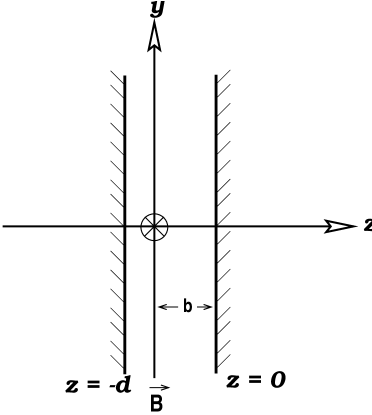
FIG. 2.: Emission by an excited three level atom in between two conducting plates. The magnetic field is along the $y$ direction. The conducting plates lead to the anisotropy of the vacuum field.

REFERENCES

- [1] P. Zhou and S. Swain, Phys. Rev. Lett. 77, 3995 (1996); Phys. Rev. A 56, 3011 (1997). P. Zhou and S. Swain, Phys. Rev. Lett. 78, 832 (1997); C.H. Keitel, ibid., 83, 1307 (1999).
- [2] E. Paspalakis and P. L. Knight, Phys. Rev. Lett. 81, 293 (1998); E. Paspalakis, N. J. Kylstra, and P. L. Knight, ibid., 82, 2079 (1999).
- [3] S.Y. Zhu and M. O. Scully, Phys. Rev. Lett. 76, 388 (1996) H. Lee, P. Polynkin, M. O. Scully, and S.Y. Zhu, Phys. Rev. A 55, 4454 (1997); F. Li and S. -Y. Zhu, ibid., 59, 2330 (1999).
- [4] H.-R. Xia, C. Y. Ye, and S.-Y. Zhu, Phys. Rev. Lett. 77, 1032 (1996); for a physical picture see G. S. Agarwal, Phys. Rev. A 55, 2457 (1997); J. Faist, F. Capasso, C. Sirtori, K. W. West, and L. N. Pfeiffer [Nature 390, 589 (1997)] demonstrated quantum interferences in experiments where dipole matrix elements were controlled by the design of quantum well structures.
- [5] O. Kocharovskaya, et al., Found. Phys. 28, 561 (1998). G. C. Hegerfeldt and M. B. Plenio, Phys. Rev. A 46, 373 (1992); ibid., 47, 2186 (1993).
- [6] G. S. Agarwal, Quantum Optics, Springer Tracts in Modern Physics Vol. 70 (Springer, Berlin, 1974), p. 95; D. A. Cardimona, M. G. Raymer, and C. R. J Stroud Jr. J. Phys. B 15, 55 (1982); S. Menon and G. S. Agarwal, Phys. Rev. A 61, 013807 (2000).
- [7] S. E. Harris [Phys. Rev. Lett. 62, 1033 (1989)] predicted the possibility of lasing without population inversion in systems where two excited states got coupled via coupling to a common reservoir; see also A. Imamoğlu, Phys. Rev. A 40, 2835 (1989).
- [8] M.O. Scully and S.Y. Zhu, Science 281, 1973 (1998).
- [9] E. Paspalakis, S.-Q. Gong, and P. L. Knight, Opt. Commun. 152, 293 (1998).
- [10] S. Menon and G.S. Agarwal, Phys. Rev.A 57, 4014 (1998); J. Javanainen, Europhys. Lett. 17, 407 (1992).
- [11] M. A. G. Martinez, P. R. Herczfeld, C. Samuels, L. M. Narducci, and C. H. Keitel, Phys. Rev. A 55, 4483 (1997).
- [12] A. K. Patnaik and G. S. Agarwal, J. Mod. Opt. 45, 2131 (1998); Z. Ficek and T. Rudolph, Phys. Rev. A 60, R4245 (1999); P. R. Berman, Phys. Rev. A 58, 4886 (1998).
- [13] cf. G.L.J.A. Rikken and Y.A.R.R. Kessener, Phys. Rev. Lett. 74, 880 (1995); R.J.Glauber and M. Lewenstein, Phys. Rev. A43, 467 (1991); S.Scheel, L. Knöll and D.G. Welsch, ibid., 60, 4094 (1999).
- [14] S.D. Brorson and P.M.W. Skovgaard in “Optical Processes in Micro-cavities”, eds R.K. Chang and A.J. Campillo (World Scientific, Singapore, 1996) p.77.
- [15] G.S. Agarwal, Phys. Rev. A. 12, 1475 (1975).
- [16] J.P. Dowling, M.O. Scully and F. de Martini, Opt. Commun. 82, 415 (1991); F.B. Seeley, J.E. Alexander, R.W. Connatser, J.S. Conway and J.P. Dowling, Am. J. Phys. 61, 545 (1993). P.L. Knight and P.W. Milloni Opt. Comm. 9, 119 (1973).
- [17] R. Loudon, “The Quantum Theory of Light” (Clarendon Press, Oxford 1973), p. 280.
- [18] G.S. Agarwal, Phys. Rev. A 11, 230 (1975).
- [19] An interesting experiment on the absorption of black-body radiation by an atom between two plates was reported by A.G. Vaidyanathan, W.P. Spencer and D. Kleppner, Phys. Rev. Lett. 47, 1592 (1982). For measurements of frequency shifts of atoms between conducting plates see M. Marrocco, M. Weidinger, R.T. Sang and H. Walther, ibid., 81, 5784 (1998).
- [20] Such effects are also expected to be relevant to the QED effects in one -d photonic bandgap structures which form the subject of recent studies - S. Y. Zhu, Y. Yang, H. Chen, H. Zheng and M. S. Zubairy, Phys. Rev. Lett. 84, 2136 (2000); J.P. Dowling, IEEE J. Lightwave Tech. 17, 2142 (1999).