Fluctuation, Dissipation, and Entanglement:
the Classical and Quantum Theory of Thermal Magnetic Noise

Abstract.

A general theory of thermal magnetic fluctuations near the surface of conductive and/or magnetically permeable slabs is developed; such fluctuations are the magnetic analog of Johnson voltage noise. Starting with the fluctuation-dissipation theorem and Maxwell’s equations, a closed-form expression for the magnetic noise spectral density is derived. Quantum decoherence, as induced by thermal magnetic noise, is analyzed via the independent oscillator heat bath model of Ford, Lewis, and O’Connell. The resulting quantum Langevin equations yield closed-form expressions for the spin relaxation times $T_{1}$, $T_{2}$, and $T_{1\rho}$. For realistic experiments in atomic physics, quantum computing, and magnetic resonance force microcopy (MRFM), the predicted relaxation rates are rapid enough that substantial experimental care must be taken to minimize them. At zero temperature, the quantum entanglement between a spin state and a thermal reservoir is computed. The same Hamiltonian matrix elements that govern fluctuation and dissipation are shown to also govern entanglement and renormalization, and a specific example of a fluctuation-dissipation-entanglement theorem is constructed. We postulate that this theorem is independent of the detailed structure of thermal reservoirs, and therefore expresses a general thermodynamic principle.

1. Introduction

The engineering control of quantum decoherence is central to several emerging scientific goals. One such goal is the direct observation of molecular structure—in three dimensions and with single-atom resolution—by magnetic resonance force microscopy [25]. Another is the solution of otherwise intractable mathematical problems—like factoring large numbers—by quantum computing [23].

At present, the main practical obstacle to achieving these goals is that the various mechanisms that cause quantum decoherence are not yet fully cataloged and understood. In consequence, quantum-coherent experiments often reveal unexpectedly fast decoherence rates, due to unanticipated—or even previously unknown—relaxation mechanisms. Similar struggles with decoherence have occupied previous scientific generations; Orbach [20] for example reviews the forty-year struggle to achieve a reasonably comprehensive understanding of relaxation in electron spin resonance.

This article is concerned with a decoherence mechanism which is ubiquitous in quantum-coherent technologies: thermal magnetic noise. Physically speaking, thermal magnetic noise is created by the same thermal current fluctuations that create Johnson noise. Thus, thermal magnetic noise is present in any device that contains electric conductors.

We will be mainly concerned with practical engineering aspects of thermal magnetic noise, but we will also give an explicit example—the first in the literature to our knowledge—of a fluctuation-dissipation-entanglement theorem. Such theorems may be broadly defined as invertible functional relations between the dissipative kernel of a system and the system’s quantum entanglement with a thermal reservoir, such that the entanglement determines the dissipation and vice versa.

This article is organized as follows. Prior work relating to thermal magnetic noise is reviewed in Section 1.1. The main new results are summarized in Section 2, these results consist of closed-form expressions for the magnetic noise spectral density (Section 2.1), quantum decoherence (Section 2.2), and a fluctuation-dissipation-entanglement theorem (Section 2.3). The practical implications of these results for quantum-coherent engineering are discussed in Section 3 via worked examples for trapped atom experiments (Section 3.1), magnetic resonance force microscopy (Section 3.2), and quantum computing (Section 3.3). Some topics for further research are suggested in Section 4.

Algebraically tedious derivations are relegated to three appendices. Appendix A derives a closed-form expression for the magnetic noise spectral density, Appendix B derives quantum Langevin and Bloch equations that describe decoherence in the presence of thermal magnetic noise, and Appendix C derives fluctuation-dissipation-entanglement theorems for both spin-$\tfrac{1}{2}$ particles and harmonic oscillators, as well as relations between dissipation and renormalization.

1.1. Prior work relating to thermal magnetic noise

The quantum field theory of electromagnetic fluctuations in lossy linear media is presented in textbooks by Landau, Lifshitz, and Piaevskii [12] and by Rytov et al. [22]. Far from a warm body, this theory describes fluctuations which are simply the familiar phenomenon of black-body radiation. Near to a warm body, the situation is considerably more complex. Non-radiating terms in the field theory become important, and create phenomena such as the Casimir force (identical to the Van der Waals force), which is familiar from chemistry and force microscopy. Recently, Dorofeyev et al. [4] have observed the attractive, fluctuating and dissipative components of the Casimir force, which were in good agreement with field-theoretic predictions.

The Casimir force arises mainly from fluctuating electric fields, which do not directly couple to the spin magnetic moments. Our investigation instead focuses on thermal fluctuations in magnetic fields.

To the best of our knowledge, the theory and experiments of Varpula and Poutanen [26], as reviewed and extended by Nenonen, Montonen, and Katila [19], were the first experimental observation and theoretical analysis of thermal magnetic fluctuations. Their work focussed on biomagnetism experiments, in which magnetic fluctuations originate in the copper walls of shielded rooms; such noise can be easily large enough to obscure biomagnetic signals. They presented a phenomenological model of thermal magnetic noise in which metallic conductors were modeled as collections of independent thermally excited resistive elements. The resulting predictions were in excellent accord with experiment.

Quantum-coherent technologies operate in a vastly different regime from biomagnetism experiments. Ambient temperatures $T$ are as low as is experimentally feasible—a few Kelvins down to millikelvins—and observation frequencies $\omega$ are megahertz to gigahertz, such that $\hbar\omega\gg k_{\mathrm{B}}T$.

Quantum-coherent phenomena dominate this physical regime. The applicability of the Varpula-Poutanen noise model then becomes uncertain, because the model is derived from a purely phenomenological description of thermal noise in room-temperature conductors. We have therefore sought to improve and extend the Varpula-Poutanen model in five respects:

1. Rigorous quantum mechanical and thermodynamic foundations have been provided via the fluctuation-dissipation theorem.

2. The results now encompass superconducting materials and/or materials with non-vanishing magnetic susceptibility.

3. A closed-form expression for the thermal magnetic noise spectral density has been obtained.

4. Bloch equations describing quantum decoherence have been derived via a quantum Langevin formalism and the independent oscillator heat bath model of Ford, Lewis, and O’Connell[6].

5. Fluctuation-dissipation-entanglement theorems have been constructed, and the link between dissipation and renormalization has been clarified.

In carrying through this program, we have been able to prove that the Varpula-Poutanen model is exact in the physical regime relevant to biomagnetism: real conductivity, macroscopic length scales, and large temperature. This explains why the Varpula-Poutanen model yields predictions which are in excellent accord with experimental measurements of biomagnetism [26], and is a tribute to their pioneering physical insight.

2. Physical motivation and main results

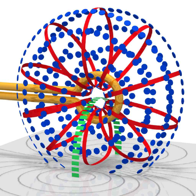
Figure 2. The B-field, E-field, and intra-slab currents—drawn to accurate scale—created by external excitation of a finite-sized current loop, as specified by (A.23–A.24). The field geometry has a ready physical interpretation: the coil excitation current generates a B-field (solid ribbons), whose time-rate-of change induces a toroidal E-field (circumferential dashed ribbons), that in turn induces currents within the slab (streamlines on the slab surface) which create a return flux loop (broad dashed ribbon) linking the induced slab currents back to the coil. The return flux induces a phase-lagged coil voltage equivalent to that of a resistive impedance, thus ensuring that the energy externally supplied to excite the coil balances the energy dissipated in the slab.

The necessary existence of thermal magnetic noise can be deduced by considering a loop antenna held near a conducting slab, as shown in Fig. 2. If a voltmeter is placed across the terminals of such an antenna, a fluctuating voltage $V(t)$ will be observed. The spectral density $S_{V}(\omega)$ of this Johnson noise is related to the complex antenna impedance $Z(\omega)$ by the well-known equation [12]

(2.1) $$S_{V}(\omega) =\text{Re}\big{(}Z(\omega)\big{)}\ \hbar\omega\coth\left(\dfrac{\hbar\omega}{2k_{\text{B}}T}\right),$$ in general;

$$\simeq\text{Re}\big{(}Z(\omega)\big{)}\ 2k_{\text{B}}T, k_{\text{B}}T\gg\hbar\omega$$ for .

Here $\text{Re}\big{(}Z(\omega)\big{)}$ is the resistive impedance. This result is just the fluctuation-dissipation theorem as it applies to fluctuating voltages in dissipative impedances.

Now we ask, what is the physical origin of these voltage fluctuations? We suppose that the coil has negligible intrinsic resistance, in which case the voltage can only have been induced by a magnetic flux threading the antenna loop. In turn, this magnetic flux can only have been generated by thermally excited currents in the nearby conducting slab.

So wherever Johnson noise is present, thermal magnetic noise will be present also, because the same underlying current fluctuations generate both phenomena.

2.1. Thermal magnetic spectral densities

We will begin by presenting closed-form expressions for the spectral density of thermal magnetic noise, and discussing their physical significance. Deriving these expressions is tedious, and is deferred until Appendix A.

Since the thermal magnetic field $\boldsymbol{B}(t)$ is a vector, its autocorrelation $\boldsymbol{C_{B}}(\tau)$ and spectral density $\boldsymbol{S_{B}}(\omega)$ are matrix-valued functions defined by

(2.2) $$\boldsymbol{C_{B}}(\tau) =\langle\boldsymbol{B}(0)\boldsymbol{\otimes}\boldsymbol{B}(\tau)\rangle,$$

(2.3) $$\boldsymbol{S_{B}}(\omega) =\int_{-\infty}^{\infty}\!e^{-i\omega\tau}\,\boldsymbol{C_{B}}(\tau)\,d\tau$$

where $$\boldsymbol{\otimes} (\boldsymbol{a}\boldsymbol{\otimes}\boldsymbol{b})_{ij}\equiv a_{i}b_{j} \boldsymbol{S_{B}}(\omega)$$ denotes the outer product of two vectors: . As shown in Section A.3, is of the general form:

(2.4) $$\boldsymbol{S_{B}}(\omega) =\boldsymbol{\Gamma}(\omega)\hbar\omega\coth\left(\dfrac{\hbar\omega}{2k_{\text{B}}T}\right)$$

$$=\big{[}\boldsymbol{I}+\boldsymbol{\hat{n}}\boldsymbol{\otimes}\boldsymbol{\hat{n}}\big{]}\,\Gamma(\omega)\hbar\omega\coth\left(\dfrac{\hbar\omega}{2k_{\text{B}}T}\right)$$

where $\boldsymbol{\hat{n}}$ is the unit vector normal to the slab surface and $\boldsymbol{I}$ is the 3$\times$3 identity matrix.

The magnetic dissipation tensor $\boldsymbol{\Gamma}(\omega)$ in (2.4) plays the same fundamental role that resistance plays in Johnson noise, in the sense that—as we will see—knowledge of $\boldsymbol{\Gamma}(\omega)$ quantitatively determines a broad spectrum of fluctuation, dissipation, and quantum entanglement phenomena.

2.1.1. Device parameters

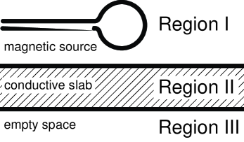
Figure 1. Conductive slab geometry. For a realistic rendition of B-field and E-field geometry, see Fig. 2. This figure defines Regions I, II, and III as referenced in (A.11).

In general, we will concerned with thermal magnetic noise induced at a distance $d$ from a conductive slab of thickness $t$, as illustrated in Fig. 1. The slab is assumed to have a frequency-dependent complex conductivity $\sigma(\omega)$ and permeability $\mu(\omega)$; for compactness we suppress the frequency-dependence of $\sigma$ and $\mu$. All results are presented in S.I. units, and all time-dependence is assumed to be $e^{i\omega t}$. See Section A.3 for a statement of Maxwell’s equations in this convention.

The four device parameters $\{d,t,\sigma,\mu\}$ may be regarded as fundamental; all other parameters are derived from them. The single most important derived parameter is the skin depth $\lambda\equiv|\omega\mu\sigma|^{-1/2}$. Another important derived parameter is the phase $\phi$ of the complex conductivity, as defined by $\boldsymbol{j}=\sigma\boldsymbol{E}=|\sigma|e^{-i\phi}$, where $\boldsymbol{E}$ is the E-field and $\boldsymbol{j}$ is the current.

2.1.2. Superconductors

For the special case of an ideal superconductor, the London equation can be stated in the form $i\mu_{0}\omega\boldsymbol{j}=\lambda_{\text{\tiny L}}^{2}\boldsymbol{E}$, where $\lambda_{\text{\tiny L}}$ is the London penetration depth. Comparing this with the definition of the conductivity $\boldsymbol{j}=\sigma\boldsymbol{E}$, we see that for an ideal superconductor $\sigma=-i\lambda_{\text{\tiny L}}^{2}/(\mu_{0}\omega)$, $\lambda=\lambda_{\text{\tiny L}}$, and $\phi=\pi/2$. Thus ideal superconductors do not have infinite conductivity, but rather have a wholly imaginary conductivity.

Real superconductors approximate ideal superconductors only at zero temperature. At finite temperatures a mixture of superconducting and normal phase charge carriers is present, such that the conductivity has an intermediate phase $\phi\in(0,\pi/2)$. See [3] for a review of the literature, including measurements of $\sigma$ at finite temperature.

2.1.3. Single paramagnetic or diamagnetic conducting slabs

Most nonferrous metals and insulators have relative magnetic permeability $K\equiv\mu/\mu_{0}\simeq 1$, where $\mu$ is the permeability of the material (the slab in our case), and $\mu_{0}$ is the permeability of the vacuum. In Appendix A we derive the following asymptotic dependance of the magnetic dissipation for $K=1$

(2.5) $$\Gamma(\omega)=\dfrac{\mu_{0}^{2}\,\text{Re}(\sigma)}{64\pi}\times\begin{cases}\dfrac{t}{d(t+d)},&\lambda\gg\text{min}\{d,\sqrt{dt}\};\\[10.76385pt] \dfrac{3\lambda^{3}}{d^{4}\,\cos(\pi/4-\phi/2)},&\lambda\ll\text{min}\{d,t\};\\[10.76385pt] \dfrac{2\lambda^{4}(dt-8\lambda^{2}\sin\phi)}{d^{5}t^{2}}.&t\ll\lambda\ll\sqrt{dt}.\end{cases}$$

Collectively, these three limits span the entire $\{d,t,\sigma,\omega\}$ design space. The following expression smoothly interpolates all three limits:

(2.6) $$\Gamma(\omega)\simeq\ \frac{3\mu_{0}^{2}\,\text{Re}(\sigma)\lambda^{3}t\cos\phi}{64\pi\big{(}3\lambda^{3}d(d+t)+(1-e^{-\alpha_{\text{c}}})td^{2}(d+2\lambda)^{2}\cos(\pi/4-\phi/2)\big{)}}.$$

It is constructed by adding the first and second asymptotic limits of (2.5) inversely, then introducing a transition parameter

(2.7) $$\alpha_{\text{c}}=(dt+8\lambda^{2}\sin\phi)/(2d\lambda\cos(\pi/4-\phi/2))$$

such that the third asymptotic limit also is smoothly interpolated.

A numerical survey shows that the resulting closed-form expression (2.6) predicts noise levels that are no more than $1.75\text{ dB}$ too large and $0.5\text{ dB}$ too small everywhere in $\{d,t,\sigma,\omega\}$ design space—an accuracy which suffices for almost all practical design work.

2.1.4. The case of two conducting slabs

The case of magnetic fluctuations measured at a point midway between two identical conducting slabs is also solved in Appendix A, and the resulting asymptotic expressions are precisely double those given in (2.5). A numerical survey shows that doubling the one-slab noise yields a slight overestimate of the two-slab midpoint noise, but the error is no more than $0.6\text{~{}dB}$ for all $\{d,t,\sigma,\omega\}$. Thus, to a very good approximation two adjacent slabs each generate independent noise at the midpoint.

2.1.5. The general case

In the general case in which both lossy magnetic permeability and electric conductivity are combined with a skin depth $\lambda$ comparable to $d$, no analytic results are presently available. Appendix A presents a one-dimensional integral (A.18) which must be numerically evaluated to determine the magnetic spectral densities.

2.1.6. Comparison with experiment

Although our general integral expression (A.18) is superficially of a different form than the Varpula-Poutanen model [26], and is derived from a very different underlying model, a numerical comparison shows that these two models yield identical predictions in the physical regime relevant to biomagnetic experiments: real conductivity, audio frequencies, vanishing magnetic susceptibility, and large temperature. Since in this regime the Varpula-Poutanen model has been shown to agree very well with experiment, we may regard the model presented in this article as having been at least partially validated.

More extensive comparisons of our model with the Varpula-Poutanen model are not feasible, because the V-P model does not contain parameters corresponding to the magnetic susceptibility $\mu$, conductivity phase $\phi$, or the quantum of action $\hbar$.

We note also that no model of thermal magnetic noise has yet been experimentally tested at microscopic scales, low temperatures, and high frequencies, in materials that are wholly or partially superconducting, or are magnetic—which is precisely the regime of greatest importance to quantum-coherent engineering.

2.2. Quantum decoherence

Now we turn our attention to the quantum decoherence induced by thermal magnetic fields. We assume a two-state system coupled to the magnetic thermal field $\boldsymbol{B}(t)$ via the Hamiltonian

$$H=-\gamma\big{(}\boldsymbol{B}_{0}+\boldsymbol{B}(t)\big{)}\boldsymbol{\cdot}\boldsymbol{s}$$

where $\gamma$ is the gyromagnetic ratio of the spin, $\boldsymbol{B}_{0}$ is a constant polarizing field, and the spin angular momentum $\boldsymbol{s}$ satisfies the usual commutation relations $[s_{i},s_{j}]=i\hbar\epsilon_{ijk}\,s_{k}$.

Our results will be expressed in terms of the rotating-frame magnetic spectral density $\boldsymbol{S}_{\boldsymbol{B}_{\text{rot}}}(\omega)$, which is given in terms of the laboratory-frame density $\boldsymbol{S}_{\boldsymbol{B}}(\omega)$ (2.4) via

(2.8) $$\boldsymbol{S}_{\boldsymbol{B}_{\text{rot}}}(\omega)=\big{(}\boldsymbol{\hat{b}}\boldsymbol{\otimes}\boldsymbol{\hat{b}}\big{)}\ \text{tr}\big{[}\boldsymbol{\hat{b}}\boldsymbol{\otimes}\boldsymbol{\hat{b}}\boldsymbol{\cdot}\boldsymbol{S}_{\boldsymbol{B}}(\omega)\big{]}+\\ \qquad\big{(}\boldsymbol{I}-\boldsymbol{\hat{b}}\boldsymbol{\otimes}\boldsymbol{\hat{b}}\big{)}\ \frac{1}{2}\,\text{tr}\big{[}(\boldsymbol{I}-\boldsymbol{\hat{b}}\boldsymbol{\otimes}\boldsymbol{\hat{b}})\boldsymbol{\cdot}\boldsymbol{S}_{\boldsymbol{B}}(\omega_{0})\big{]},$$

where the precession frequency $\omega_{0}$ about the unit axis of spin precession $\boldsymbol{\hat{b}}$ is given by $\gamma\boldsymbol{B}_{0}\equiv\omega_{0}\boldsymbol{\hat{b}}$, and $\text{tr}[\ldots]$ is the matrix trace (the sum of diagonal elements).

In Appendix B we derive the quantum Langevin equations for a spin-$\tfrac{1}{2}$ particle coupled to a thermal magnetic field, and from them we show that the time evolution of the spin density matrix is described by Bloch-type equations with relaxation times $T_{1}$, $T_{2}$, and $T_{1\rho}$ given by

(2.9a) $$\frac{1}{T_{1}} =\frac{1}{2}\,\gamma^{2}\,\text{tr}\big{[}(\boldsymbol{I}-\boldsymbol{\hat{b}}\boldsymbol{\otimes}\boldsymbol{\hat{b}})\boldsymbol{\cdot}\boldsymbol{S}_{\boldsymbol{B}_{\text{rot}}}(0)\big{]}$$

(2.9b) $$\frac{1}{T_{2}} =\frac{1}{2T_{1}}+\frac{1}{2}\gamma^{2}\,\text{tr}\big{[}\boldsymbol{\hat{b}}\boldsymbol{\otimes}\boldsymbol{\hat{b}}\boldsymbol{\cdot}\boldsymbol{S}_{\boldsymbol{B}_{\text{rot}}}(0)\big{]}$$

(2.9c) $$\frac{1}{T_{1\rho}} =\frac{1}{2}\,\gamma^{2}\,\text{tr}\big{[}(\boldsymbol{I}-\boldsymbol{\hat{b}}_{1}\boldsymbol{\otimes}\boldsymbol{\hat{b}}_{1})\boldsymbol{\cdot}\boldsymbol{S}_{\boldsymbol{B}_{\text{rot}}}(\omega_{1})\big{]}$$

Here $T_{1\rho}$ is the relaxation time in the presence of a radio-frequency (RF) applied field—commonly called a “spin-locking” field. In the frame co-rotating with the RF field, it appears as a constant B-field $\boldsymbol{B}_{1}=B_{1}\boldsymbol{\hat{b}}_{1}$ whose characteristic precession frequency is $\omega_{1}=\gamma B_{1}$. Substituting (2.4–2.8) in (2.9a–2.9b), we obtain $\{T_{1},T_{2},T_{1\rho}\}$ explicitly in terms of the magnetic damping coefficient $\Gamma(\omega)$ given in (2.6)

(2.10a) $$\frac{1}{T_{1}} =\frac{1}{2}\,\gamma^{2}\,(3-\cos^{2}\theta)\,\Gamma(\omega_{0})\,\hbar\omega_{0}\,\coth\left(\frac{\hbar\omega_{0}}{2k_{\text{B}}T}\right)$$

(2.10b) $$\frac{1}{T_{2}} =\frac{1}{2T_{1}}+\frac{1}{2}\gamma^{2}(1+\cos^{2}\theta)\,\Gamma(0)\,2k_{\text{B}}T$$

(2.10c) $$\frac{1}{T_{1\rho}} =\frac{1+\cos^{2}\beta}{2T_{1}}+$$

$$\quad\quad\quad\frac{1}{2}\gamma^{2}\sin^{2}\!\beta\ (1+\cos^{2}\theta)\,\Gamma(\omega_{1})\,\hbar\omega_{1}\,\coth\left(\frac{\hbar\omega_{1}}{2k_{\text{B}}T}\right)$$

Here $\cos\theta=\boldsymbol{\hat{b}}\boldsymbol{\cdot}\boldsymbol{\hat{n}}$ and $\cos\beta=\boldsymbol{\hat{b}}\boldsymbol{\cdot}\boldsymbol{\hat{b}}_{1}$, where $\boldsymbol{\hat{b}}_{1}$ is the RF field axis in the rotating frame, $\boldsymbol{\hat{b}}$ is the polarization axis, and $\boldsymbol{\hat{n}}$ is the unit vector normal to the slab surface.

Note that $\Gamma(\omega)$ appears with varying frequency arguments $\omega\in\{0,\omega_{1},\omega_{0}\}$; this has important design consequences because in most cases $\Gamma(\omega)$ exhibits a strong frequency dependence.

As far as practical quantum engineering is concerned, expressions (2.10a–2.10c) are the main “deliverable” of this article.

2.3. A fluctuation-dissipation-entanglement theorem

From a purely formal point of view, fluctuation-dissipation-entanglement theorems exist for a simple reason: the same Hamiltonian matrix elements that control fluctuation and dissipation also control certain measures of quantum entanglement; Appendix C discusses this point of view.

Physically speaking, we reason as follows. We consider a two-state quantum system, which—as in the real world—interacts weakly with a thermal reservoir. We adjust the temperature of the reservoir to zero, and ask: what is the probability that the two-state system is not in its ground state? To the extent that this probability is non-zero, it describes an irreducible quantum entanglement with the thermal reservoir.

Now, at zero temperature the classical entanglement probability is zero, and even the Bloch equations (B.19), which have a firmer quantum justification, relax spin systems to their ground state at zero temperature, and thus predict zero entanglement.

However, a higher-order calculation reveals that the entanglement probability is finite even at zero temperature. We calculate this probability as follows. As before, we consider a spin-$\tfrac{1}{2}$ particle magnetically coupled to a thermal reservoir. We polarize the spin via an external field $\boldsymbol{B}_{0}$, which lifts the degeneracy of the spin system along a polarization axis $\omega_{0}\boldsymbol{\hat{p}}=\gamma\boldsymbol{B}_{0}$, with $\gamma$ the gyromagnetic ratio of the spin and $\omega_{0}$ the (by convention positive) precession frequency. We let $|\psi_{0}\rangle$ be the ground state of the isolated spin, and we define a projection operator $P_{\mathcal{E}}=\mathbb{I}-|\psi_{0}\rangle\boldsymbol{\otimes}\langle\psi_{0}|$, with $\mathbb{I}$ the identity operator. By construction, the expectation value of $P_{\mathcal{E}}$ vanishes for an isolated ground state: $\langle\psi_{0}|P_{\mathcal{E}}|\psi_{0}\rangle=0$.

Of course, no real-world spin system is perfectly isolated. We therefore enlarge our Hilbert space to encompass a thermal reservoir with a potentially infinite set of basis states $\{|\phi_{i}\rangle;i\in 0,1,\ldots,\infty\}$. We generalize $P_{\mathcal{E}}$ to include the thermal reservoir by defining a new projection operator $\mathcal{E}$

(2.11) $$\mathcal{E}\equiv\sum_{i}|\phi_{i}\rangle\otimes P_{\mathcal{E}}\otimes\langle\phi_{i}|$$

which projects onto the subspace in which the spin is not in its ground state.

It is a well-defined problem to calculate, perturbatively, the expectation $\langle\Psi_{0}|\mathcal{E}|\Psi_{0}\rangle$, where $|\Psi_{0}\rangle$ the ground state of the combined spin-plus-thermal-reservoir system. Keeping in mind that $\mathcal{E}$ and $|\Psi_{0}\rangle$ depend on $\boldsymbol{\hat{p}}$ and $\omega_{0}$, we can define a scalar entanglement function $E(\boldsymbol{\hat{p}},\omega_{0})\equiv\langle\Psi_{0}|\mathcal{E}|\Psi_{0}\rangle$. In Appendix C we show that $E(\boldsymbol{\hat{p}},\omega_{0})$ is related to the magnetic dissipation tensor $\boldsymbol{\Gamma}(\omega)$ by the following fluctuation-dissipation-entanglement theorem:

(2.12) $$E(\boldsymbol{\hat{p}},\omega_{0}) =\frac{\gamma^{2}\hbar}{4\pi}\ \text{\large$\mathfrak{G}$}_{2}\big{\{}\omega\,\text{tr}\big{[}(\boldsymbol{I}-\boldsymbol{\hat{p}}\boldsymbol{\otimes}\boldsymbol{\hat{p}})\boldsymbol{\cdot}\boldsymbol{\Gamma}(\omega)\big{]};\omega_{0}\big{\}}$$

Here $\mathfrak{G}_{2}$ is a Stieltj i e s transform, in Bateman’s notation [2], as defined by

(2.13) $$\text{\large$\mathfrak{G}$}_{\!\rho}\{f(x);y\}=\int_{0}^{\infty}\!\!dx\ f(x)(x+y)^{-\rho}$$

We note that Stieltj i e s transforms are invertible, such that a measurement of the entanglement function $E(\boldsymbol{\hat{p}},\omega_{0})$ suffices in principle to determine the magnetic dissipation tensor $\boldsymbol{\Gamma}(\omega)$ and vice versa.

For practical quantum engineering purposes, the main utility of this theorem is that it allows us to determine the hard-to-measure entanglement from the easier-to-measure (or predict) dissipation. For the particular case of thermal magnetic noise, the frequency dependence (2.6) of $\boldsymbol{\Gamma}(\omega)$ is such that the Stieltj i e s integral is absolutely convergent, so that the entanglement of real-world devices can be readily be calculated.

2.3.1. Approximate expression for the entanglement

In general, the Stieltj i e s integral (2.12) cannot be evaluated in closed form. However, a simple and physically meaningful approximate evaluation is possible. We begin by remarking that dissipative kernels always have a cut-off frequency $\omega_{\text{c}}$, because otherwise their associated noise spectral density would carry infinite power. For the particular case of thermal magnetic noise originating in a thick plate, the cut-off frequency is such that $\lambda(\omega_{\text{c}})\sim d$. We assume the frequency of interest $\omega_{0}$ is small compared to the cut-off frequency, so that $\omega_{\text{c}}\gg\omega_{0}$, and we brutally approximate $\boldsymbol{\Gamma}(\omega)$ as constant over the range $\omega\in(\omega_{0},\omega_{\text{c}})$, and zero elsewhere. Then the Stieltj i e s integral (2.12) can be evaluated in closed form as

(2.14) $$E(\boldsymbol{\hat{p}},\omega_{0}) \simeq\frac{\gamma^{2}\hbar}{4\pi}\,\text{tr}\big{[}(\boldsymbol{I}-\boldsymbol{\hat{p}}\boldsymbol{\otimes}\boldsymbol{\hat{p}})\boldsymbol{\cdot}\boldsymbol{\Gamma}(\omega_{0})\big{]}\,\ln(\omega_{\text{c}}/\omega_{0})$$ from (2.12)

$$=\frac{\gamma^{2}\hbar}{4\pi}\,\text{tr}\big{[}(\boldsymbol{I}-\boldsymbol{\hat{p}}\boldsymbol{\otimes}\boldsymbol{\hat{p}})\boldsymbol{\cdot}\frac{\boldsymbol{S}_{\boldsymbol{B}}(\omega_{0})}{\hbar\omega_{0}}\big{]}\,\ln(\omega_{\text{c}}/\omega_{0}) T\to 0$$ by (2.4) for

$$=\frac{\ln(\omega_{\text{c}}/\omega_{0})}{2\pi\omega_{0}T_{1}}$$ by (2.8) and (2.9a)

where $T_{1}$ is evaluated at zero temperature.

3. Quantum engineering implications

We will now apply (2.4–2.10) in the design analysis of representative quantum technologies. Our goal is partly to illustrate practical applications of our results, and partly to identify areas where further research is needed.

A small but important point: when quoting numerical values $\propto 1/\sqrt{\text{\small Hz}}$ we shall embrace the usual engineering convention that bandwidths encompass only positive frequencies; this requires the insertion of an additional factor of two when evaluating two-sided spectral densities, e.g. (2.4).

3.1. Atom and ion traps

We begin by considering thermal magnetic noise at centimeter length scales and audio frequencies, at room temperature. This is the same regime considered by Varpula and Poutanen [26, 19], and it is also a regime typical of at least some atomic physics experiments [8].

Specifically, we will calculate the spectral density of the thermal magnetic fields between room-temperature two copper slabs, each $t=1\ \text{cm}$ thick, spaced $2d=2\ \text{cm}$ apart. We are particularly interested in the zero-frequency spectral density in the $\boldsymbol{\hat{n}}$ direction normal to the slab surface, because this describes thermally induced fluctuations in the background polarizing field. At room temperature $T=300\ \text{K}$ the conductivity of high-purity copper is of order $5.9\times 10^{7}\ (\Omega\text{\ m})^{-1}$. From (2.4) and (2.6), with $d=t=1\ \text{cm}$ and $\phi=0$, and taking into account that we have two plates whose noise is additive, we find at zero frequency $(\boldsymbol{\hat{n}}\boldsymbol{\cdot}\boldsymbol{S}_{\boldsymbol{B}}(0\,\text{Hz})\boldsymbol{\cdot}\boldsymbol{\hat{n}})^{1/2}\sim 1.2\ \text{pT}/\sqrt{\text{\small Hz}}$, rolling off to $(\boldsymbol{\hat{n}}\boldsymbol{\cdot}\boldsymbol{S}_{\boldsymbol{B}}(100\,\text{Hz})\boldsymbol{\cdot}\boldsymbol{\hat{n}})^{1/2}\sim 0.6\ \text{pT}/\sqrt{\text{\small Hz}}$ at 100 Hertz.

Until recently, such picoTesla fluctuations would have been viewed as being of no practical consequence. However, magnetic fields change sign under time reversal, and hence magnetic fluctuations locally violate time-reversal invariance, and so these fluctuations must be understood and controlled in high-precision tests of fundamental physics.

For example, the most stringent experimental limit on the electric dipole moment $d_{\text{\tiny E}}$ of a fundamental particle is $d_{\text{\tiny E}}\leq 8.7\times 10^{-28}\ \text{$e$ cm}$ for the mercury isotope ${}^{199}\text{Hg}$ [8] (here $e$ is the electron charge). Typically, dipole moments are measured by observing the change in precession frequency induced by an applied electric field of magnitude $E$. It follows that $\boldsymbol{S}_{\boldsymbol{B}}$ can be expressed as an equivalent dipole noise spectral density $S_{d}=(\hbar\gamma/(2E))^{2}\,\boldsymbol{\hat{n}}\boldsymbol{\cdot}\boldsymbol{S}_{\boldsymbol{B}}(0)\boldsymbol{\cdot}\boldsymbol{\hat{n}}$. For ${}^{199}\text{Hg}$, the gyromagnetic ratio $\gamma/(2\pi)=7.59\ \text{MHz/Tesla}$. This yields a zero-frequency equivalent dipole noise for our example of room-temperature copper plates of

$$ES_{d}^{1/2}\sim 1.94\times 10^{-20}\ \text{eV}/\sqrt{\text{\small Hz}}.$$

For a typical electric field $E\sim 10^{4}\ \text{V/cm}$, the equivalent dipole noise would therefore be $S_{d}^{1/2}\sim 1.94\times 10^{-24}\ \text{$e$ cm}/\sqrt{\text{\small Hz}}$.

This is a substantial noise level: it would naively require an averaging time on the order of $10^{7}$ seconds to better the published electric dipole moment limit [8]. And it would not be entirely straightforward to reduce the thermal magnetic noise by making the copper shields thinner or less conductive, because this would defeat their purpose of shielding the experiment from external fields.

Fortunately, another effect provides mitigation: trapped atom experiments typically measure the net signal from atoms in many different regions of a cell. To the extent that $n$ independent regions are averaged, the equivalent dipole noise power will be reduced by a factor of $1/n$. Some of the formalism necessary for calculating $n$ is set forth in Appendix A.1. Detailed calculations would be strongly dependent on the particular design chosen.

3.2. Magnetic resonance force microscopy

Magnetic resonance force microscopy (MRFM) is a quantum-coherent technology whose ultimate objective is to produce magnetic resonance images of individual molecules in situ, nondestructively, in three dimensions, with Angstrom resolution. Such a technology would allow much of molecular biology to be conducted as an observational science—along the lines of, e.g., astronomy—rather than an experimental science.

We remark that a single-spin MRFM imaging device can be alternatively regarded as a first-generation solid-state quantum computer, in which the individual qubits carry binary information about the presence or absence of a spin spin at a specified atomic coordinate.

There are two main experimental challenges in MRFM. The first is that single-spin signal forces are exceedingly small, of order $10^{-18}\,\text{N}$ for electron magnetic moments. The MRFM community’s design options for achieving the required sensitivity are reasonably well understood (but challenging to implement in practice): reduce the mass of the cantilever, increase its damping time, reduce the ambient temperature, and employ a sharper magnetic tip with a higher field gradient.

The second—emerging—challenge in MRFM is that the spin state must maintain its quantum coherence for a time long enough to detect the signal force. Here the design issues are not yet well understood. We will illustrate some of these issues by calculating the effects of thermal magnetic noise on spin relaxation in a typical MRFM environment.

We model the magnetic tip as a sphere with radius $r=1\,\mu\text{m}$ and uniform magnetization $\mu_{0}M=1\ \text{T}$. The electron magnetic moment is located at a separation $d=50\ \text{nm}$ from the tip surface. At this distance the polarizing field is $B_{0}=2\mu_{0}Mr^{3}/(3(r+d)^{3})=0.58\ \text{T}$, and the spin precession frequency is $\gamma B_{0}/(2\pi)=16.1\ \text{GHz}$, where $\gamma/(2\pi)=2.8\ \text{MHz}/T$ is the gyromagnetic ration of the electron. We take the ambient temperature to be $T=4\ \text{K}$. We note that $d\ll r$ and we therefore—roughly—model the tip as a slab of thickness $t=d$. Finally, the direction of the polarizing field is taken to be parallel to the vector normal to the tip suface ($\theta=0$).

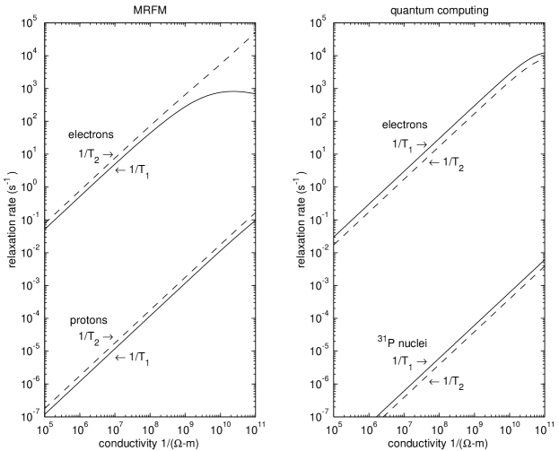
Figure 3. Predicted spin relaxation rates in magnetic resonance force microscopy and in quantum computing, as a function of conductivity.

With the parameters $\{d,t,T,\gamma,\omega_{0},\theta\}$ now specified (see Section 2.1.1 for further discussion), the electron spin relaxation rates $1/T_{1}(\sigma)$ and $1/T_{2}(\sigma)$ are predicted as functions of the tip conductivity $\sigma$ by expressions (2.10a–2.10b), with results as shown in Fig. 3. For completeness, relaxation times for proton magnetic moments at the same distance from the tip are also shown.

3.2.1. Design lessons for MRFM

It is clear that tip conductivity is a key engineering parameter in MRFM. For example, if the tip conductivity is as great as that of pure elemental iron ($\sim 4\times 10^{9}\ \Omega\text{-m}$ at $4\ \text{K}$) or nickel ($\sim 1.7\times 10^{10}\ \Omega\text{-m}$ at $4\ \text{K}$), the predicted relaxation rate is $1/T_{1}\gtrsim 10^{2}\ \text{s}^{-1}$. Such rates are much too rapid to permit coherent spin imaging.

Real-world MRFM tips typically are composed not of pure elements, but of magnetically “hard” alloys such as samarium-cobalt or neodymium-iron-boron. These alloys are commerically prepared as powders, without much regard for minimizing lattice defects: the resulting conductivity is very likely to be substantially reduced relative to the values quoted above for pure elements. There is not much data in the literature relating to the electrical conductivity of ferromagnetic particles at cryogenic temperature. Misra et al. [17] have measured the conductivity of sputtered Cu/Cr multilayered films to be $\sim 2.5\times 10^{-7}\ \Omega\text{-m}$ in the zero-temperature limit. If we take this value to be representative of micron-scale ferromagnetic tips at cryogenic temperatures—in the absence of better data—the predicted relaxation rate is $1/T_{1}\sim 10\ \text{s}^{-1}$. This is still an uncomfortably rapid relaxation rate.

If these predictions are correct, the MRFM community has at least five design options: (1) reduce the temperature, (2) reduce the tip conductivity (e.g., by employing an insulating magnetic garnet tip), (3) employ superconducting tips (e.g., generating gradients via trapped vortices), (4) detect electron moments incoherently, or (5) focus on coherent proton detection, for which the predicted relaxation times are much longer.

We see how vital it is to achieve a thorough understanding of all the mechanisms that influence spin relaxation. It is sobering, therefore, to reflect upon some of the thermal reservoirs that we have not mentioned, which surely are present in ferromagnetic tips: spin waves, thermally excited domain wall motions, and unpaired electron spins in passivating oxide layers, to name three. As discussed in Section 4, much work remains to be done.

3.3. Quantum computing

Kane [9] has described a design for a solid-state quantum computer in which the qubits are the electron and nuclear spin quantum numbers of ${}^{31}\text{P}$ donor sites in a silicon lattice. Now we will consider the effects of thermal magnetic noise within Kane’s device.

In Kane’s design, the ${}^{31}\text{P}$ donor sites carry both nuclear and electron quantum numbers, which are coupled by a Hamiltonian $H_{\text{int}}$ of the form

(3.1) $$H_{\text{int}}=\gamma_{\text{e}}\boldsymbol{B}_{0}\boldsymbol{\cdot}\boldsymbol{s}_{\text{e}}+\gamma_{\text{n}}\boldsymbol{B}_{0}\boldsymbol{\cdot}\boldsymbol{s}_{\text{n}}+4\hbar^{-2}\!A\,\boldsymbol{s}_{\text{e}}\boldsymbol{\cdot}\boldsymbol{s}_{\text{n}}$$

Here $\boldsymbol{s}_{\text{e}}$ and $\boldsymbol{s}_{\text{n}}$ are the electron and ${}^{31}\text{P}$ spin operators, $\gamma_{\text{e}}$ and $\gamma_{\text{n}}$ are the gyromagnetic ratios (in a convention where both ratios are positive), and the hyperfine coupling $A$ has the value $\hbar A/(2\pi)=29\ \text{MHz}$.

The computational action occurs between the two lowest energy levels of this system, and the presence of the hyperfine coupling modifies these lowest-energy levels in two respects. First, the energy separation of the two levels depends on $A$ via an equation given by Kane as

(3.2) $$\hbar\omega_{0}=\gamma_{\text{n}}B_{0}+2A+\mathcal{O}(A^{2})$$

Second, the two lowest energy levels of the system couple to external time-dependent B-fields $\boldsymbol{B}_{\text{ext}}(t)$ via an effective Hamiltonian $H_{\text{eff}}$ which a straightforward perturbative calculation shows to be

(3.3) $$H_{\text{eff}}=\frac{\hbar\gamma_{\text{n}}}{2}\,\boldsymbol{B}_{\text{ext}}(t)\boldsymbol{\cdot}\boldsymbol{K}\boldsymbol{\cdot}\boldsymbol{\sigma}$$

where $\boldsymbol{\sigma}\equiv\{\sigma_{x},\sigma_{y},\sigma_{z}\}$ is a vector of Pauli matrices acting on the two lowest-energy states, and $\boldsymbol{K}$ is a dimensionless matrix given by

(3.4) $$\boldsymbol{K}=\boldsymbol{\hat{b}}\boldsymbol{\otimes}\boldsymbol{\hat{b}}+\left(1+\frac{2A}{\gamma_{\text{n}}B_{0}}\right)\big{(}\boldsymbol{I}-\boldsymbol{\hat{b}}\boldsymbol{\otimes}\boldsymbol{\hat{b}}\big{)}+\mathcal{O}(A^{2})$$

where $\boldsymbol{\hat{b}}$ is a unit vector in the direction of the applied B-field. We observe that the hyperfine coupling $A$ acts to increase the coupling of the two lowest-energy states to thermal magnetic noise. This increased coupling is most conveniently taken into account by the replacement in (2.8) of the laboratory-frame spectral density $\boldsymbol{S}_{\boldsymbol{B}}$ by an effective spectral density $\boldsymbol{S}_{\boldsymbol{B}}^{\text{eff}}$

(3.5) $$\boldsymbol{S}_{\boldsymbol{B}}\rightarrow\boldsymbol{S}_{\boldsymbol{B}}^{\text{eff}}\equiv\boldsymbol{K}\boldsymbol{\cdot}\boldsymbol{S}_{\boldsymbol{B}}\boldsymbol{\cdot}\boldsymbol{K}$$

Subsequent calculations of relaxation rates are unaltered. In Kane’s design, the renormalized coupling $\boldsymbol{K}$ increases the predicted relaxation rates by a factor of order $\left(1+(2A)/(\gamma_{\text{n}}B_{0})\right)^{2}\sim 7.2\,$.

Per Kane’s design [9], we specify a polarizing field $B_{0}=2\ \text{T}$ and a temperature $T=100\ \text{mK}$. We model Kane’s A-gates and J-gates as metallic pads of thickness $t=5\ \text{nm}$ at a distance $d=10\ \text{nm}$ from the ${}^{31}\text{P}$ centers. The direction of the polarizing field is taken to be parallel to the vector normal to the pad surface ($\theta=0$). The electron-spin and nuclear-spin relaxation rates $1/T_{1}$ and $1/T_{2}$ are then predicted as functions of the pad conductivity $\sigma$ by expressions (2.10a–2.10b), with results as shown in Fig. 3.

3.3.1. Design lessons for solid-state quantum computing

Kane’s article optimistically quotes the magnetic resonance literature to the effect

at temperatures $T\sim 1.5\ \text{K}$ the electron spin relaxation time is thousands of seconds, and […] at millikelvin temperatures the phonon limited ${}^{31}\text{P}$ relaxation time is of the order of $10^{18}$ seconds, making this system ideal for quantum computation.

We see that thermal magnetic noise originating in the A- and J-gates is likely to substantially increase these relaxation rates. Fortunately, to the extent that calculation occurs only between the two lowest-energy states, the predicted rapid relaxation of the higher-energy electron states may not pose a problem. And it is gratifying that the predicted ${}^{31}\text{P}$ relaxation rates remain reasonably small even when the amplifying effects of the hyperfine coupling are taken into account.

These predictions should be regarded very cautiously, however. As we discuss at greater length in the following section, even the notion of conductivity becomes suspect at these length scales and temperatures. In our view, the main design lesson is that all potential noise sources must be treated seriously.

4. Conclusions

We have developed a general theory of thermal magnetic fluctuations near the surface of conductive and/or magnetically permeable slabs. We have applied the resulting closed-form expression for the magnetic spectral density (Section 2.1) to practical problems in atomic physics experiments, magnetic resonance force microscopy, and solid-state quantum computing (Sections 3.1–3.3). The theory predicts magnetic noise levels that are large enough to require substantial care to minimize their effects.

More generally, our formalism indicates that if the dissipative kernel of a linearly damped system is known, then the consequences for fluctuation, dissipation, entanglement, and renormalization are fully determined, via fluctuation-dissipation theorems (eqs. (2.4) and (C.9)), fluctuation-dissipa- tion-entanglement theorems (eqs. (2.12) and (C.10)), and renormalization-dissipation relations (eqs. (C.14) and (C.15)).

We postulate that these fluctuation-dissipation-entanglement-renormaliz-ation relations are universal, in the sense that they apply to all thermal reservoirs, without regard for the internal structure of the reservoir, with the sole restriction that the coupling to the reservoir must be weak enough to be linearly dissipative.

A major limitation of our article is that we derived our results in the context of a specific model of thermal reservoirs—the independent oscillator (IO) model—and hence we have not proved universality. Ford, Lewis, and O’Connell’s pioneering article on independent oscillator models [6] proves universality in the restricted sense that these models are shown to describe all forms of fluctuation and dissipation that are causal and linearly dissipative. An important milestone for further research would be to prove universality in an expanded context which included entanglement and renormalization in addition to fluctuation and dissipation.

There are also substantial reasons to expect that measurement processes might also be subsumed under a suitably expanded notion of universality. We reason as follows. Quantum-coherent technologies necessarily include some means for reading-out binary data; in quantum computing the data are qubits, in MRFM experiments the data are the presence or absense of a spin at a given atomic coordinate. In most cases measurement is a continuous interferometric process, achieved e.g. via weak interactions of a cantilever with laser-supplied photons. From an engineering point of view, the measurement photons comprise a “good” reservoir—effectively at zero temperature—whose finely tuned interactions compete with many different “bad” thermal reservoirs that contribute only noise. The quantum system seeks to achieve equilibrium with the “good” and “bad” reservoirs simultaneously; the resulting quantum dynamics are traditionally described by master equations of the Fokker-Planck type. A unified formalism of this sort, treating measurement and noise processes on a common footing, would offer many practical advantages in quantum-coherent engineering.

In carrying through these calculations, we have come to appreciate an emerging common ground—the technical challenge of preserving and manipulating quantum coherence—that is shared by magnetic resonance force microscopy and quantum computation. Single-spin MRFM imaging devices (if they can be demonstrated) would constitute first-generation solid-state quantum computers, in which the individual qubits carried binary information about the presence or absence of a spin spin at a specified atomic coordinate.

Arguably the most daunting challenge in developing quantum-coherent technologies is achieving simultaneous engineering control of a panoply of thermal reservoirs:

• phonons and surface vibrational modes

• ferro- and ferrimagnetic spin waves and domain walls

• conduction band excitations in metals and semiconductors

• paramagnetic and nuclear spins

• mobile molecules and charges on surfaces

• lattice defects and impurities

• super-conducting condensates admixed with normal-phase conductors

This list includes most of the excitations that are commonly studied by condensed matter physicists. We remark it is not enough to achieve good engineering control of some or even most of these noise sources; all must be controlled simultaneously, as even one poorly-controlled noise source is enough to destroy quantum coherence.

The dissipative kernels of these excitations are poorly understood at the ultra-low temperatures and mesoscopic length scales that are characteristic of quantum-coherent technologies. For example, even Maxwell’s equations in conducting media—an exceedingly well-studied area of physics—will require re-interpretation due to our still-limited understanding of mesoscopic conductivity [13, 7].

In view of these difficulties, Landauer has modestly proposed [14] that the following disclaimer be appended to all quantum computing proposals:

This proposal, like all proposals for quantum computation, relies upon speculative technology, does not in its current form take into account all possible sources of noise, unreliability and manufacturing error, and probably will not work.

Our article may be read as a response to Landauer’s concerns: we have analyzed thermal magnetic noise as a “possible source of noise and unreliability” in MRFM imaging and in Kane’s proposal for a quantum computer. More ambitiously, we have done so in the context of a general formalism which might be applied across a broad range of thermal reservoirs. In doing so, we hope to have contributed to the emerging task of providing solid and well-organized foundations for the development of quantum-coherent technologies.

Appendix A Fluctuation and dissipation

Many readers will be acquainted with the fluctuation-dissipation theorem as it applies to voltage noise—known as Johnson noise—in resistive circuit elements [12]. The theorem can be briefly stated as follows: if a net charge $q(t)=qe^{i\omega t}$ is passed through a frequency-dependent impedance $Z(\omega)$, such that the current $i(t)=\partial q(t)/\partial t=i\omega qe^{i\omega t}$, and the power $P(\omega)$ dissipated in the impedance is $P(\omega)=\text{Re}(Z(\omega))\,q^{2}\omega^{2}$, then the spectrum of thermal voltage fluctuations is given in terms of the dissipative impedance $\text{Re}(Z)$ by (2.1).

The general fluctuation-dissipation theorem allows us to deduce, by an exact analogy, that if a time-dependent magnetic moment $\boldsymbol{m}(t)=\boldsymbol{m}\,e^{i\omega t}$ is adjacent to a conductive slab, such that the power dissipated in the slab is $P=\boldsymbol{m}\boldsymbol{\cdot}\boldsymbol{\Gamma}(\omega)\boldsymbol{\cdot}\boldsymbol{m}\,\omega^{2}$, then the spectrum of the magnetic fluctuations is given in terms of the magnetic dissipation matrix $\boldsymbol{\Gamma}(\omega)$ via (2.4).

Discussions which justify the above line of reasoning are presented in many graduate-level textbooks [11, 1], but these discussions tend to be rather abstract and lengthy. Some readers will prefer the following physical derivation, which is completely general and rigorous.

We will deduce the spectrum of magnetic fluctuations from the well-known spectrum of thermal voltage fluctuations [12] (Johnson noise).

Let $A$ be the area of the pickup loop in Fig. 2, and let $\boldsymbol{\hat{m}}$ be the unit vector normal to the loop. We let $I$ and $\boldsymbol{m}$ be the real coefficients of the loop current $I(t)=Ie^{i\omega t}$ and loop magnetic moment $\boldsymbol{m}(t)=\boldsymbol{m}e^{i\omega t}$, such that $\boldsymbol{m}=AI\boldsymbol{\hat{m}}$. We wish to compute the spectral density $\boldsymbol{\hat{m}}\boldsymbol{\cdot}\boldsymbol{S}_{\boldsymbol{B}}\boldsymbol{\cdot}\boldsymbol{\hat{m}}$ of the magnetic field traversing the loop. We reason as follows:

$$\boldsymbol{\hat{m}}\boldsymbol{\cdot}\boldsymbol{S}_{\boldsymbol{B}}\boldsymbol{\cdot}\boldsymbol{\hat{m}}\ \begin{array}[t]{ll}=\ S_{\Phi}/A^{2},&\text{magnetic flux $\Phi=A\,\boldsymbol{\hat{m}}\boldsymbol{\cdot}\boldsymbol{B}$};\\[4.30554pt] =\ S_{V}/(\omega A)^{2},&\text{Faraday's law of Induction;}\\[4.30554pt] =\ \text{Re}(Z)/(\omega A)^{2}\ 2k_{\text{B}}T,&\text{thermal voltage noise per \eqref{eq:RNoise};}\\[4.30554pt] =\ P/(\omega IA)^{2}\ 2k_{\text{B}}T,&\text{because $P=\text{Re}(Z)I^{2}$;}\\[4.30554pt] =\ \boldsymbol{m}\boldsymbol{\cdot}\boldsymbol{\Gamma}\boldsymbol{\cdot}\boldsymbol{m}/(IA)^{2}\ 2k_{\text{B}}T,&\text{definition of $\boldsymbol{\Gamma}$ in terms of $P$;}\\[4.30554pt] =\ \boldsymbol{\hat{m}}\boldsymbol{\cdot}\boldsymbol{\Gamma}\boldsymbol{\cdot}\boldsymbol{\hat{m}}\ 2k_{\text{B}}T,&\text{substitute $\boldsymbol{m}=IA\,\boldsymbol{\hat{m}}$.}\end{array}$$

Since the result holds for arbitrary loop orientation $\boldsymbol{\hat{m}}$, and both $\boldsymbol{S}_{\boldsymbol{B}}$ and $\boldsymbol{\Gamma}$ are symmetric matrices, it must be that $\boldsymbol{S}_{\boldsymbol{B}}(\omega)=\boldsymbol{\Gamma}(\omega)\,2k_{\text{B}}T$, QED.

A.1. Spatial correlations and gradients

This reasoning is readily extended to encompass spatial correlations and gradients. Let $n$ magnetic moments $[\boldsymbol{m}]\equiv\{\boldsymbol{m}_{1},\boldsymbol{m}_{2},\ldots,\boldsymbol{m}_{n}\}$ be located at coordinates $\{\boldsymbol{x}_{1},\boldsymbol{x}_{2},\ldots,\boldsymbol{x}_{n}\}$. Assuming a time dependence $\propto e^{i\omega t}$, the dissipated power is calculable from the geometry and conductivity of the system—at least in principle—and will be of the general form $P=[\boldsymbol{m}]\boldsymbol{\cdot}\left[\boldsymbol{\Gamma}\right]\boldsymbol{\cdot}[\boldsymbol{m}]\,\omega^{2}$, where $\left[\boldsymbol{\Gamma}\right]$ is the obvious $n$–point generalization of $\boldsymbol{\Gamma}$. Then the $n$–point generalization of (2.4) is simply

(A.1) $$\boldsymbol{S}_{[\boldsymbol{B}]}=\left[\boldsymbol{\Gamma}\right]\,\hbar\omega\coth\left(\dfrac{\hbar\omega}{2k_{\text{B}}T}\right)$$

In this fashion all questions involving $n$–point spectral densities of magnetic noise can be reduced to the calculation of $\left[\boldsymbol{\Gamma}\right]$. Although we will not do so in this article, the spectral density of magnetic gradients can be determined by considering the limiting case in which two coordinates approach each other.

A.2. Classical and quantum calculations

Students in particular may be troubled that our calculation of the dissipation tensor $\boldsymbol{\Gamma}(\omega)$ will be entirely classical, via Maxwell’s equations. After all, doesn’t the title of this article promise “the classical and quantum theory of thermal magnetic noise”? The quantum part of the promise will be fullfilled in Appendix B, to follow, in which we present a rigorous quantum theory of a spin coupled to a thermal reservoir, and show that the classical dissipative kernel determines the quantum dissipation also.

A.3. Solving the Maxwell equations

To calculate power dissipation within the slab, and thus determine $\boldsymbol{\Gamma}(\omega)$, we seek solutions of Maxwell’s equations in their standard form for time dependence $\propto e^{i\omega t}$ [21]:

(A.2) $$\boldsymbol{\nabla}\boldsymbol{\times}\boldsymbol{E} =-i\omega\boldsymbol{B} \boldsymbol{\nabla}\boldsymbol{\cdot}\boldsymbol{D} =\rho_{\text{c}}$$

$$\boldsymbol{\nabla}\boldsymbol{\times}\boldsymbol{H} =\boldsymbol{j}+i\omega\boldsymbol{D} \boldsymbol{\nabla}\boldsymbol{\cdot}\boldsymbol{B} =0$$

together with the constitutive and divergence equations for the current

(A.3) $$\boldsymbol{j} =(\sigma\boldsymbol{E}+\boldsymbol{j}^{\text{s}}) \boldsymbol{\nabla}\boldsymbol{\cdot}\boldsymbol{j} =-i\omega\rho_{\text{c}}$$

Here $\boldsymbol{B}$ is the magnetic field, $\boldsymbol{H}=\boldsymbol{B}/\mu$ is the magnetic intensity, $\mu$ is the magnetic permeability, $\boldsymbol{E}$ is the electric field, $\boldsymbol{D}=\epsilon\boldsymbol{E}$ is the electric displacement, $\boldsymbol{j}$ is the total current, $\epsilon$ is the electric permittivity, $\rho_{\text{c}}$ is the charge density, $\sigma$ is the conductivity, and $\boldsymbol{j}^{\text{s}}$ is the externally-applied dipole source current.

A.3.1. The scalar Maxwell equations

We begin our solution of the Maxwell equations with the help of a simplifying ansatz: that the irrotational part of $\boldsymbol{E}$ and $\boldsymbol{D}$ vanishes, i.e., the charge density $\rho_{\text{c}}$ is zero within the slabs and at their interfaces. Furthermore, we will assume that the displacement current $i\omega\boldsymbol{D}=i\omega\epsilon\boldsymbol{E}$ is negligibly small compared to the conduction current $\sigma\boldsymbol{E}$. This approximation is quite accurate for all the cases we will consider, e.g., for room temperature copper at one GHz we have $\omega\epsilon/\sigma\sim 10^{-9}$.

It is natural to write a divergence-free $\boldsymbol{E}$ field as a curl; we write $\boldsymbol{E}$ as

(A.4a) $$\boldsymbol{E}=-i\omega\,\boldsymbol{\nabla}\boldsymbol{\times}(\psi\boldsymbol{\hat{n}})$$

where $$\psi \boldsymbol{\hat{n}} \boldsymbol{\nabla}\boldsymbol{\cdot}\boldsymbol{D}=0 \psi \boldsymbol{\nabla}\boldsymbol{\times}\boldsymbol{E}=-i\omega\boldsymbol{B}$$ is a scalar vorticity, and we recall that is the (constant) unit vector normal to the slab surfaces. Per our ansatz, (A.4a) guarantees that everywhere within a slab (boundary conditions will be considered shortly). In terms of , the Maxwell equation becomes

(A.4b) $$\boldsymbol{B}=\boldsymbol{\hat{n}}\,(\nabla^{2}\psi)-\boldsymbol{\nabla}(\boldsymbol{\hat{n}}\boldsymbol{\cdot}\boldsymbol{\nabla}\psi)$$

which, furthermore, guarantees $$\boldsymbol{\nabla}\boldsymbol{\cdot}\boldsymbol{B}=0 \boldsymbol{\nabla}\boldsymbol{\times}\boldsymbol{H}=\sigma\boldsymbol{E}+\boldsymbol{j}^{\text{s}}$$. The sole remaining Maxwell equation is then equivalent to the scalar wave equation

(A.4c) $$\nabla^{2}\psi=i\mu\sigma\psi+j^{\text{s}}$$

where $$j^{\text{s}}$$ is a scalar dipole source whose nature will be specificed shortly.

It remains only to enforce the usual boundary conditions of electrodynamics: continuity of the normal components of $\boldsymbol{B}$ and $\boldsymbol{D}$ and the transverse components of $\boldsymbol{E}$ and $\boldsymbol{H}$. These are equivalent to the following boundary conditions on $\psi$ at the juncture of two slabs $i$ and $j$

(A.4d) $$\psi_{i} =\psi_{j}$$

(A.4e) $$(\boldsymbol{\hat{n}}\boldsymbol{\cdot}\boldsymbol{\nabla}\psi_{i})/\mu_{i} =(\boldsymbol{\hat{n}}\boldsymbol{\cdot}\boldsymbol{\nabla}\psi_{j})/\mu_{j}$$

The problem is now reduced to the solution of the scalar wave equation (A.4c), subject to the between-slab boundary conditions (A.4d). The $\boldsymbol{E}$ and $\boldsymbol{B}$ fields are given by (A.4a) and (A.4b), which now are purely constitutive equations.

A.3.2. The scalar dipole source

For a (vector) magnetic dipole $\boldsymbol{m}$ located within a region of zero conductivity, it is convenient to specify the scalar source $j^{\text{s}}$ implicitly by $j^{\text{s}}=\nabla^{2}\psi^{\text{s}}$, with the source field $\psi^{\text{s}}$ given by

(A.5) $$\psi^{\text{s}}(\boldsymbol{x})=\frac{\mu}{4\pi}\,\left(\frac{\boldsymbol{\hat{n}}}{|\boldsymbol{x}|}+\frac{\boldsymbol{\hat{x}}\cdot(\boldsymbol{I}-\boldsymbol{\hat{n}}\otimes\boldsymbol{\hat{n}})}{|\boldsymbol{x}|+\boldsymbol{x}\cdot\boldsymbol{\hat{n}}}\right)\cdot\boldsymbol{m}$$

Inserting $\psi^{\text{s}}$ in the constitutive equation (A.4b) yields for $\boldsymbol{B}$

(A.6) $$\boldsymbol{B}(\boldsymbol{x})=\frac{\mu}{4\pi|\boldsymbol{x}|^{3}}\,(3\,\boldsymbol{\hat{x}}\otimes\boldsymbol{\hat{x}}-\boldsymbol{I})\cdot\boldsymbol{m}$$

which (by construction) is the dipole B-field generated by a magnetic moment $\boldsymbol{m}$. This justifies our specification of $\psi^{\text{s}}$ as the source field. The possibility of writing a general dipole field in this form is the key step leading to the success of our scalar ansatz.

As a technical point, the vector potential $\psi^{\text{s}}(\boldsymbol{x})\boldsymbol{\hat{n}}$ describes an E-field which is singular along a line extending from $\boldsymbol{x}=0$ to infinity in the $-\boldsymbol{\hat{n}}$ direction (away from the slab). As we will show in Section A.3.6, the singular portion of the E-field is irrotational, and it can be written as the gradient of a harmonic potential which disappears when we introduce a finite charge density on the surface of the slab. The dissipated power within the slab is not appreciably affected by the currents required to create this surface charge, so for the time being the singularity can simply be ignored.

A.3.3. Solving the scalar Maxwell equations

The scalar equation (A.4c) for $\psi$ is most easily solved in cylindrical coordinates $\{r,\varphi,z\}$. It is further convenient to work with the Bessel transform $\tilde{\psi}_{m}(\rho,z)$ defined by

(A.7) $$\tilde{\psi}_{m}(\rho,z)=\frac{1}{2\pi}\int_{0}^{2\pi}\!d\varphi\int_{0}^{\infty}\!r\,dr\,\,e^{-im\varphi}J_{m}(\rho r)\,\psi(r,\varphi,z)$$

whose inverse is

(A.8) $$\psi(r,\varphi,z)=\sum_{m=-\infty}^{m=\infty}e^{im\varphi}\int_{0}^{\infty}\!d\rho\,\rho\,J_{m}(\rho r)\tilde{\psi}_{m}(\rho,z)$$

Here $J_{m}$ is a Bessel function of integer argument. The scalar wave equation for $\tilde{\psi}_{m}(\rho,z)$ is

(A.9) $$\frac{\partial^{2}}{\partial z^{2}}\tilde{\psi}_{m}(\rho,z)=i\omega\mu\sigma\tilde{\psi}_{m}(\rho,z)+\tilde{j}_{m}^{\text{s}}(\rho,z)$$

whose general homogenous solution is

(A.10) $$\tilde{\psi}_{m}(\rho,z)=\tilde{\psi}^{+}_{m}(\rho)e^{kz}+\tilde{\psi}^{-}_{m}(\rho)e^{-kz}$$

where we have introduced the complex wavenumber $k\equiv\sqrt{i\omega\mu\sigma+\rho^{2}}$.

Our next task is to explicitly solve for the Bessel coefficients $\tilde{\psi}_{m}(\rho)$. We divide space into three regions {I,II,III}, where Region I is the nonconductive region that contains the dipole source, Region II is the conductive slab of thickness $t$ beginning at a distance $d$ from the source, and Region III is the nonconducting region on the opposite side of the slab (see Fig. 1).

Within Regions I and III we assume vanishing conductivity $\sigma=0$ and a purely real permeability $\mu_{0}$. In contrast, within Region II we allow both $\sigma$ and $\mu$ to assume complex values. Thus energy dissipation can occur only within Region II.

Requiring that $\tilde{\psi}_{m}(\rho,z)\to 0$ as $|z|\to\infty$ leads to the general solution:

(A.11) $$\tilde{\psi}_{m}(\rho,z)=\left\{\begin{array}[]{ccl}\tilde{\psi}^{\text{I}{+}}_{m}(\rho)e^{\rho z}+\tilde{\psi}^{\text{s}}_{m}(\rho,z)&&\text{Region I (source);}\\ \parbox[c]{120.00018pt}{\dotfill}&|&{\scriptstyle\ z=d}\\ \tilde{\psi}^{\text{II}{+}}_{m}(\rho)e^{kz}+\tilde{\psi}^{\text{II}{-}}_{m}(\rho)e^{-kz}&\!\!+z\!\!&\text{Region II (slab);}\\ \parbox[c]{120.00018pt}{\dotfill}&\downarrow&{\scriptstyle\ z=d+t}\\ \tilde{\psi}^{\text{III}{-}}_{m}(\rho)e^{-\rho z}&&\text{Region III (far side).}\end{array}\right.$$

For illustrations of Regions I, II, and III, see Figs. 1–2. The source term $\tilde{\psi}^{\text{s}}_{m}(\rho,z)$ in Region I is found by substituting (A.5) in (A.7):

(A.12) $$\tilde{\psi}^{\text{s}}_{0}(\rho,z) =\frac{\mu_{0}}{4\pi\rho}\,e^{-\rho|z|}\boldsymbol{\hat{n}}\boldsymbol{\cdot}\boldsymbol{m}$$

(A.13) $$\tilde{\psi}^{\text{s}}_{\pm 1}(\rho,z) =\frac{\mu_{0}}{8\pi\rho}\,e^{-\rho|z|}\,(\boldsymbol{\hat{x}}\pm i\boldsymbol{\hat{y}})\boldsymbol{\cdot}\boldsymbol{m}$$

where we have introduced Cartesian basis vectors $\boldsymbol{\hat{x}}\boldsymbol{\times}\boldsymbol{\hat{y}}=\boldsymbol{\hat{n}}$. Note the singularity at $z=0$; this reflects our assumption of a point dipole source. Section A.3.6 derives explicitly nonsingular expressions for $\boldsymbol{B}$ and $\boldsymbol{E}$ originating from finite-sized current sources, however the present dipole result is adequate for our main purpose of estimating power dissipation in the slab.

With the source term now specified, the boundary equations (A.4d) for the Bessel coefficients $\{\tilde{\psi}^{\text{I}{+}}_{0},\tilde{\psi}^{\text{II}{+}}_{0},\tilde{\psi}^{\text{II}{-}}_{0},\tilde{\psi}^{\text{III}{-}}_{0}\}$ can be readily solved. We obtain for the $m=0$ coefficients:

(A.14) $$\left[\begin{matrix}\tilde{\psi}^{\text{I}{+}}_{0}\\[2.15277pt] \tilde{\psi}^{\text{II}{+}}_{0}\\[2.15277pt] \tilde{\psi}^{\text{II}{-}}_{0}\\[2.15277pt] \tilde{\psi}^{\text{III}{-}}_{0}\end{matrix}\right]=\frac{\mu_{0}}{4\pi}\ \left[\begin{matrix}e^{-2\rho d}(e^{2kt}-1)(K^{2}\rho^{2}-k^{2})\\[2.15277pt] -2e^{-(\rho+k)d}(K\rho-k)K\rho\\[2.15277pt] 2e^{2kt-(\rho-k)d}(K\rho+k)K\rho\\[2.15277pt] 4e^{(\rho+k)}kK\rho\end{matrix}\right]\times\\ \frac{\boldsymbol{\hat{n}}\boldsymbol{\cdot}\boldsymbol{m}}{\rho\big{(}(K^{2}\rho^{2}+k^{2})(e^{2kt}-1)+2K\rho k(e^{2kt}+1)\big{)}}$$

where $K\equiv\mu/\mu_{0}$ is the relative permeability of the slab. The $m=\pm 1$ coefficients are directly proportional to the $m=0$ coefficients

(A.15) $$\left[\begin{matrix}\tilde{\psi}^{\text{I}{+}}_{\pm 1}\\ \vdots\end{matrix}\right] =\frac{(\boldsymbol{\hat{x}}\pm i\boldsymbol{\hat{y}})\boldsymbol{\cdot}\boldsymbol{m}}{2(\boldsymbol{\hat{n}}\boldsymbol{\cdot}\boldsymbol{m})}\left[\begin{matrix}\tilde{\psi}^{\text{I}{+}}_{0}\\ \vdots\end{matrix}\right]$$

When we calculate magnetic spectral densities, this simple proportionality will ensure that $\boldsymbol{\Gamma}\propto(\boldsymbol{I}+\boldsymbol{\hat{n}}\boldsymbol{\otimes}\boldsymbol{\hat{n}})$ at all frequencies and length scales.

A.3.4. Energy dissipation

Our next task is to calculate the power $P$ dissipated within Region II. From classical electrodynamics we have

(A.16) $$P =\int_{V}\!\!dV\ \left(\boldsymbol{j}\boldsymbol{\cdot}\boldsymbol{E}+\boldsymbol{H}\boldsymbol{\cdot}\frac{\partial\boldsymbol{B}}{\partial t}\right)$$

which with the help of the Bessel orthogonality relations becomes

(A.17) $$P =2\pi\!\!\!\sum_{m=-\infty}^{\infty}\int_{0}^{\infty}\!\!\!\rho\,d\rho\int_{d}^{d+t}\!\!\!\!dz\ \left(\rho^{2}\omega^{2}\text{Re}(\sigma)+\rho^{4}\omega\frac{\text{Im}(\mu)}{|\mu|^{2}}\right)\ |\psi_{m}(\rho,z)|^{2}$$

Carrying through the $z$-integration, we find the scalar magnetic dissipation coefficient $\Gamma(\omega)$, as implicitly defined by $P\equiv\omega^{2}\Gamma(\omega)\,\big{(}\boldsymbol{m}\boldsymbol{\cdot}(\boldsymbol{I}+\boldsymbol{\hat{n}}\boldsymbol{\otimes}\boldsymbol{\hat{n}})\boldsymbol{\cdot}\boldsymbol{m}\big{)}$ :

(A.18) $$\Gamma(\omega)=\frac{\mu_{0}^{2}}{4\pi}\int_{0}^{\infty}\!\!d\rho\ \left(\rho^{3}\text{Re}(\sigma)+\frac{\rho^{5}\text{Im}(\mu)}{\omega|\mu|^{2}}\right)\ |K|^{2}e^{-2\rho d}\times\\ \frac{\text{Re}\left[ik^{\ast}(e^{2kt}-1)(e^{2k^{\ast}t}+1)(K^{2}\rho^{2}-k^{2})/(\omega\mu\sigma)+\rho K|e^{2kt}-1|^{2}\right]}{\big{|}(K^{2}\rho^{2}+k^{2})(e^{2kt}-1)+2K\rho k(e^{2kt}+1)\big{|}^{2}}$$

where we recall that $k\equiv\sqrt{i\omega\mu\sigma+\rho^{2}}$ and $K\equiv\mu/\mu_{0}$. In simplifying this result we have kept only the leading and next-to-leading terms in $\text{Im}(\mu)$, i.e., we have assumed $K$ is predominantly real.

The case of thermal magnetic fluctuations measured at a point midway between two identical conducting slabs can be solved by exactly similar methods. It is only necessary to replace the Region I homogenous term $\tilde{\psi}^{\text{I}{+}}_{m}(\rho)e^{\rho z}$ in (A.11) with the symmetrized term $\tilde{\psi}^{\text{I}{+}}_{m}(\rho)\cosh(\rho z)$. The resulting magnetic dissipation coefficient is

(A.19) $${\Gamma^{\prime}}(\omega)=\frac{\mu_{0}^{2}}{4\pi}\int_{0}^{\infty}\!\!d\rho\ \left(\rho^{3}\text{Re}(\sigma)+\frac{\rho^{5}\text{Im}(\mu)}{\omega|\mu|^{2}}\right)\ |K|^{2}e^{-2\rho d}\times\\ \frac{2\text{Re}\left[ik^{\ast}(e^{2kt}-1)(e^{2k^{\ast}t}+1)(K^{2}\rho^{2}-k^{2})/(\omega\mu\sigma)+\rho K|e^{2kt}-1|^{2}\right]}{\big{|}(k^{2}+K^{2}\rho^{2}+e^{-2\rho d}(k^{2}-K^{2}\rho^{2}))(e^{2kt}-1)+2K\rho k(e^{2kt}+1)\big{|}^{2}}$$

Note that the double-slab integrand is just twice the single-slab integrand, slightly modified by an additional term $\propto e^{-2\rho d}$ in the denominator. For the special case $K=1$ (the case of primary interest) this additional term can be shown to be non-leading for all values of $\{\rho,d,t,\sigma,\omega\}$. A numerical survey confirms that ${\Gamma^{\prime}}(\omega)\simeq 2\Gamma(\omega)$ to within very good accuracy, as described in Section 2.1.

A.3.5. Asymptotic limits for paramagnetic and diamagnetic slabs

The three asymptotic expressions in (2.5) are obtained by evaluating (A.18) for $K=1$ and $\text{Im}(\mu)=0$ in the following limits:

(A.20) $$\Gamma(\omega)\simeq\text{Re}(\sigma)\,\frac{\mu_{0}^{2}}{4\pi}\int_{0}^{\infty}\!\!\!\!d\rho\times\!\begin{cases}\dfrac{(1-e^{-2\rho t})}{8e^{2\rho d}},&\text{$|\sigma|\to 0$;}\\[10.76385pt] \dfrac{\rho^{3}\lambda^{3}e^{-2\rho d}}{2\cos(\pi/4-\phi/2)},&\text{$|\sigma|\to\infty$;}\\[10.76385pt] \dfrac{\rho^{3}\lambda^{4}(t-4\rho\lambda^{2}\sin\phi)}{t^{2}e^{2\rho d}},&kt\ll 1\ll\rho d.\end{cases}$$

The integrations are readily carried out, with the results as in (2.5).

A.3.6. The irrotational electric field

Now we have only one chore remaining: repairing the irrotational singularity in the E-field mentioned in Section A.3.2, and verifying that the repair does not alter the energy dissipation just calculated. In the end, we will obtain expressions for the E- and B-fields which are closed-form and explicitly finite.

In outline, the repair is accomplished by adding a purely irrotational E-field to Region I—thereby relaxing the ansatz of Section  A.3.1 that $\boldsymbol{E}$ is purely rotational. With the added E-field, Faraday’s law $\boldsymbol{\nabla}\boldsymbol{\times}\boldsymbol{E}=-i\omega\boldsymbol{B}$ is still satisfied, because the added E-field is irrotational. Because the added field is confined to Region I, which is nonconductive, and because displacement currents $i\omega\boldsymbol{D}$ are negligibly small, Ampere’s law $\boldsymbol{\nabla}\boldsymbol{\times}\boldsymbol{H}=\sigma\boldsymbol{E}+\boldsymbol{j}^{\text{s}}+i\omega\boldsymbol{D}\simeq\boldsymbol{j}^{\text{s}}$ is still satisfied. Gauss’s law $\boldsymbol{\nabla}\boldsymbol{\cdot}\boldsymbol{D}=0$ is still satisfied because the added E-field is the gradient of a harmonic potential. Physically, the added field is generated by surface charge on the slab, and the within-slab currents necessary to sustain the surface charge are negligibly small compared to the eddy currents already computed. Thus, the added E-field does not alter the magnetic dissipation coefficient $\boldsymbol{\Gamma}(\omega)$ already computed. The remainder of this section is devoted to proving these assertions.

We begin by noting that the E-field singularity in Region I physically corresponds to the field induced by an end-to-end line of electric dipoles along the $-\boldsymbol{\hat{n}}$ axis. It is easy to verify that such a singularity can be cancelled by the addition of an (irrotational) E-field which is the gradient of the harmonic potential $\phi_{1}^{\text{I}}(\boldsymbol{x})$,

(A.21) $$\phi_{1}^{\text{I}}(\boldsymbol{x})=i\omega\,\frac{\mu_{0}}{4\pi}\,\frac{\boldsymbol{\hat{x}}\boldsymbol{\cdot}(\boldsymbol{\hat{n}}\boldsymbol{\times}\boldsymbol{m})}{|\boldsymbol{x}|+\boldsymbol{x}\cdot\boldsymbol{\hat{n}}}$$

To satisfy the boundary conditions between Regions I and II, we must also add the E-field of the image potential

(A.22) $$\phi_{2}^{\text{I}}(\boldsymbol{x})\equiv-\phi_{1}^{\text{I}}(2d\boldsymbol{\hat{n}}-\boldsymbol{x})$$

in order that $\boldsymbol{E}^{\text{I}}=\boldsymbol{\nabla}(\phi_{1}^{\text{I}}+\phi_{2}^{\text{I}})$ be normal to the slab surface, thus ensuring that the transverse component of $\boldsymbol{E}$ remains continuous at the boundary.

To sustain the $\boldsymbol{E}^{\text{I}}$, a charge density $\rho^{\text{I}}=\epsilon\boldsymbol{\hat{n}}\boldsymbol{\cdot}\boldsymbol{E}^{\text{I}}$ must exist on the surface of the slab, and this surface charge must in turn be created by a normal-to-surface current within the slab $\boldsymbol{j}^{\text{I}}=i\omega\rho^{\text{I}}\boldsymbol{\hat{n}}$. Relative to the intraslab eddy currents current $\sigma\boldsymbol{E}$ which are our main concern, it is easy to show that $\boldsymbol{j}^{\text{I}}$ is of order $\omega\epsilon/\sigma\sim 10^{-9}$ (see the discussion following (A.2)) and thus is negligible.

Putting all these pieces together, we are now ready to specify the fields in Region I in a manifestly finite manner, assuming only that the spatial size of the current source is reasonably small compared to the distance $d$ separating the source from the slab (like the current loop in Fig. 2).

From the localized current source, we compute a vector potential $\boldsymbol{A}(\boldsymbol{x})$ in the usual manner

(A.23) $$\boldsymbol{A}(\boldsymbol{x})=\frac{\mu_{0}}{4\pi}\ \int_{V}\!\!d^{3}\boldsymbol{{x^{\prime}}}\ \frac{\boldsymbol{j}(\boldsymbol{{x^{\prime}}})}{|\boldsymbol{x}-\boldsymbol{{x^{\prime}}}|}\sim\frac{\mu_{0}}{4\pi}\ \frac{\boldsymbol{m}\boldsymbol{\times}\boldsymbol{\hat{x}}}{|\boldsymbol{x}|^{2}}$$

where $\boldsymbol{j}(\boldsymbol{{x^{\prime}}})$ is the (finite) current density within the (finite) source. From the far-field limit of $\boldsymbol{A}(\boldsymbol{x})$ we determine the dipole moment $\boldsymbol{m}$ of the source, and under the assumption that the size of the source is small compared to $d$, we use $\boldsymbol{m}$ to compute the back-reaction vorticity field $\psi^{\text{I}}(\boldsymbol{x})$ via equations (A.8–A.14) and the back-reaction irrotational field $\phi_{2}^{\text{I}}$ via (A.22). With the help of the identity $-i\omega\boldsymbol{A}(\boldsymbol{x})=-i\omega\boldsymbol{\nabla}\boldsymbol{\times}(\psi^{\text{s}}(\boldsymbol{x}))+\boldsymbol{\nabla}\phi_{1}^{\text{I}}(\boldsymbol{x})$, which is exact for a point dipole current source, the net B-field and E-field in Region I can be written as follows

(A.24a) $$\boldsymbol{B}(\boldsymbol{x}) =\boldsymbol{\nabla}\boldsymbol{\times}\boldsymbol{A}(\boldsymbol{x})-\boldsymbol{\nabla}(\boldsymbol{\hat{n}}\boldsymbol{\cdot}\boldsymbol{\nabla}\psi^{\text{I}}(\boldsymbol{x}))$$

(A.24b) $$\boldsymbol{E}(\boldsymbol{x}) =-i\omega\boldsymbol{A}(\boldsymbol{x})-i\omega\boldsymbol{\nabla}\boldsymbol{\times}(\psi^{\text{I}}(\boldsymbol{x})\boldsymbol{\hat{n}})+\boldsymbol{\nabla}\phi_{2}^{\text{I}}(\boldsymbol{x})$$

where $\boldsymbol{A}(\boldsymbol{x})$, $\psi^{\text{I}}(\boldsymbol{x})$, and $\phi_{2}^{\text{I}}(\boldsymbol{x})$ are individually nonsingular.

Physically speaking, $\boldsymbol{A}(\boldsymbol{x})$ describes the E- and B-fields that are generated directly by the source current, $\psi^{\text{I}}(\boldsymbol{x})$ describes the E- and B-fields generated by the induced currents within the slab (treating the source current as a dipole), and $\phi_{2}^{\text{I}}(\boldsymbol{x})$ describes the E-field generated by surface charges on the slab (also treating the source current as a dipole). These expressions were used to generate the field geometry in Fig. 2.

Appendix B Quantum decoherence

In this section we present an exactly solvable microscopic model of a spin-$\tfrac{1}{2}$ particle magnetically coupled to a heat bath. Our goal is derive the expressions for $T_{1}$, $T_{2}$, and $T_{1\rho}$ quoted in (2.9a)-(2.9c).

We follow Ford, Lewis, and O’Connell in modeling the heat bath as a collection of independent harmonic oscillators [6]; the reader is referred to this article for a thermodynamic justification of this model. We will adjust the bath parameters so as to reproduce the known spectral density of magnetic fluctuations, which we computed in the previous section. The quantum Langevin and optical Bloch equations—which yield closed-form expressions for $T_{1}$, $T_{2}$, and $T_{1\rho}$—will then be uniquely determined.

B.1. The thermal reservoir Hamiltonian

The Hamiltonian $H$ of the spin/heat bath system is taken to be

(B.1) $$H=-\gamma\boldsymbol{B}_{0}\boldsymbol{\cdot}\boldsymbol{s}+\sum_{j}\frac{1}{2}\omega_{j}\left(p_{j}^{2}+(q_{j}-\beta_{j}\boldsymbol{\hat{n}}_{j}\boldsymbol{\cdot}\boldsymbol{s})^{2}\right)$$

Here $\boldsymbol{B}_{0}$ is the polarizing field, $\gamma$ is the gyromagnetic ratio of the spin, and $\boldsymbol{s}$ is the angular momentum operator of the spin, satisfying commutation relations $[s_{i},s_{j}]=i\hbar\epsilon_{ijk}s_{k}$. The heat bath is described in terms of oscillators with resonant frequency $\omega_{i}$, whose dynamical coodinates $\{p_{i},q_{i}\}$ satisfy $[q_{i},p_{j}]=i\hbar\delta_{ij}$, which are coupled to the spin with strength $\beta_{j}$.

The physical nature of the heat bath variables need not be otherwise specified. Reader may optionally conceive them as, e.g., thermal excitations of conduction band electrons, magnons in a ferromagnet, excited states of the vacuum in field theory, or in general as excitations of whatever heat bath is furnished by a given quantum technology.

We begin by solving the equation of motion of the heat bath variables. In the Heisenberg picture we have

(B.2) $$\ddot{q}_{j}+\omega_{j}^{2}q_{j}=\beta_{j}\omega_{j}^{2}\boldsymbol{\hat{n}}_{j}\boldsymbol{\cdot}\boldsymbol{s}$$

Following Ford et al., we write the formal solution to these equations as

(B.3) $$q_{j}(t)=q_{j}^{\text{h}}(t)+\beta_{j}\boldsymbol{\hat{n}}_{j}\boldsymbol{\cdot}\boldsymbol{s}(t)-\int_{-\infty}^{t}\!\!d{t^{\prime}}\,\cos(\omega_{j}(t-{t^{\prime}}))\,\beta_{j}\boldsymbol{\hat{n}}_{j}\boldsymbol{\cdot}\boldsymbol{\dot{s}}({t^{\prime}})$$

Here $q_{j}^{\text{h}}(t)$ is a homogenous solution to the equations of motion (corresponding physically to the evolution of the heat bath in the absence of the back-action of the spin). With the help of this result, the spin operator equation of motion $\dot{\boldsymbol{s}}=[\boldsymbol{s},H]/(i\hbar)$ can be readily cast into the form of the following quantum Langevin equation

(B.4) $$\boldsymbol{\dot{s}}(t) =-\gamma\boldsymbol{B}_{0}\boldsymbol{\times}\boldsymbol{s}(t)-$$

$$\quad\frac{1}{2}\gamma\big{(}\boldsymbol{B}(t)\boldsymbol{\times}\boldsymbol{s}(t)-\boldsymbol{s}(t)\boldsymbol{\times}\boldsymbol{B}(t)\big{)}+$$

$$\quad\frac{1}{2}\,\left[\big{(}\boldsymbol{C}\boldsymbol{\cdot}\boldsymbol{s}(t)\big{)}\boldsymbol{\times}\boldsymbol{s}(t)-\boldsymbol{s}(t)\boldsymbol{\times}\big{(}\boldsymbol{C}\boldsymbol{\cdot}\boldsymbol{s}(t)\big{)}\right]+$$

$$\quad\!\!\int_{-\infty}^{t}\!\!\!\!d{t^{\prime}}\,\frac{1}{2}\left[\big{(}\boldsymbol{G}(t-{t^{\prime}})\boldsymbol{\cdot}\boldsymbol{\dot{s}}({t^{\prime}})\big{)}\boldsymbol{\times}\boldsymbol{s}(t)-\boldsymbol{s}(t)\boldsymbol{\times}\big{(}\boldsymbol{G}(t-{t^{\prime}})\boldsymbol{\cdot}\boldsymbol{\dot{s}}({t^{\prime}})\big{)}\right]$$

Here $\boldsymbol{B}(t)$ is a fluctuating thermal magnetic field which depends only on the homogenous heat bath operators $q_{j}^{\text{h}}(t)$

(B.5) $$\boldsymbol{B}(t) =\sum_{j}\gamma^{-1}\omega_{j}\beta_{j}q_{j}^{\text{h}}(t)\boldsymbol{\hat{n}}_{j}$$

and $$\boldsymbol{G}(t-{t^{\prime}})$$ is a dissipative kernel

(B.6) $$\boldsymbol{G}(t-{t^{\prime}}) =\begin{cases}\sum_{j}\omega_{j}\beta_{j}^{2}\,\cos(\omega_{j}(t-{t^{\prime}}))\,\boldsymbol{\hat{n}}_{j}\boldsymbol{\otimes}\boldsymbol{\hat{n}}_{j}&t>{t^{\prime}}\\ 0&t<{t^{\prime}}\end{cases}$$

Note that $\boldsymbol{G}(t-{t^{\prime}})$ is a pure c-number matrix which is independent of the temperature of the heat bath. It is the matrix generalization of what Ford et al. call the “memory function” of the heat bath.

The anisotropy tensor $\boldsymbol{C}$ is a symmetric c-number tensor given by

(B.7) $$\boldsymbol{C}=\sum_{j}\omega_{j}\beta_{j}^{2}\,\boldsymbol{\hat{n}}_{j}\boldsymbol{\otimes}\boldsymbol{\hat{n}}_{j}$$

Physically speaking, $\boldsymbol{C}$ describes the interaction of the particle with image currents in the nearby slab. This reflects a very general and physically realistic property of the independent oscillator model: the dynamical equations of a particle are renormalized by its interaction with the thermal reservoir.

For the special case of spin-$\tfrac{1}{2}$ particles $\boldsymbol{C}$ has no dynamical effects, due to an identity satisfied by spin-$\tfrac{1}{2}$ operators (and not by higher-spin particles)

(B.8) $$s_{i}s_{j}+s_{j}s_{i}=\frac{\hbar^{2}}{2}\,\mathbb{I}$$

where $\mathbb{I}$ is the identity operator. This identify ensures that the $\boldsymbol{C}$-dependent terms in (B.4) vanish identically; we emphasize that this occurs only for spin-$\tfrac{1}{2}$ particles.

So far, we have not used the fact that the heat bath variables are in thermal equilibrium; we now use this fact to compute the spectral density $\boldsymbol{S}_{\boldsymbol{B}}$ of $\boldsymbol{B}(t)$. Not surprisingly, we will discover that $\boldsymbol{S}_{\boldsymbol{B}}$ has a functional form that is closely related to the dissipative kernel $\boldsymbol{G}$.

The calculation is straightforward. Denoting a thermal ensemble average by $\langle\ldots\rangle_{t}$, we follow Ford et al. in noting that the correlation of the homogenous heat bath operators $\{q_{i}^{\text{h}}\}$ is of the simple form

(B.9) $$\langle q_{i}^{\text{h}}(t)q_{j}^{\text{h}}({t^{\prime}})\rangle_{t}=\frac{1}{2}\,\delta_{ij}\,\hbar\coth\left(\frac{\hbar\omega_{j}}{2k_{\text{B}}T}\right)\,\cos(\omega_{j}(t-{t^{\prime}}))$$

Combining this with (B.5) yields an explicit expression for $\boldsymbol{S}_{\boldsymbol{B}}(\omega)$

(B.10) $$\boldsymbol{S}_{\boldsymbol{B}}(\omega) =\int_{-\infty}^{\infty}\!\!d\tau\,e^{-i\omega\tau}\frac{1}{2}\langle\boldsymbol{B}(t)\boldsymbol{\otimes}\boldsymbol{B}(t+\tau)+\boldsymbol{B}(t+\tau)\boldsymbol{\otimes}\boldsymbol{B}(t)\rangle_{t}$$

$$=\sum_{j}\frac{\omega_{j}^{2}\beta_{j}^{2}}{2\gamma^{2}}\,\boldsymbol{\hat{n}}_{j}\boldsymbol{\otimes}\boldsymbol{\hat{n}}_{j}\,\hbar\coth\left(\frac{\hbar\omega}{2k_{\text{B}}T}\right)\,\int_{-\infty}^{\infty}\!\!d{t^{\prime}}\,e^{-i\omega\tau}\cos(\omega_{j}\tau)$$

$$=\sum_{j}\frac{\pi\omega_{j}\beta_{j}^{2}}{2\gamma^{2}}\,\boldsymbol{\hat{n}}_{j}\boldsymbol{\otimes}\boldsymbol{\hat{n}}_{j}\,\hbar\omega\coth\left(\frac{\hbar\omega}{2k_{\text{B}}T}\right)\,\big{(}\delta(\omega-\omega_{j})+\delta(\omega+\omega_{j})\big{)}$$

If we compare this result with the real part of the Fourier transform of the dissipative kernel

(B.11) $$\text{Re}\,\boldsymbol{\tilde{G}}(\omega) =\text{Re}\int_{-\infty}^{\infty}\!\!d{t^{\prime}}\,e^{-i\omega(t-{t^{\prime}})}\boldsymbol{G}(t-{t^{\prime}})$$

$$=\frac{\pi}{2}\,\sum_{j}\omega_{j}\beta_{j}^{2}\,\boldsymbol{\hat{n}}_{j}\boldsymbol{\otimes}\boldsymbol{\hat{n}}_{j}\,\big{(}\delta(\omega-\omega_{j})+\delta(\omega+\omega_{j})\big{)}$$

it is apparent that

(B.12) $$\boldsymbol{S}_{\boldsymbol{B}}(\omega)=\gamma^{-2}\text{Re}\,\boldsymbol{\tilde{G}}(\omega)\,\hbar\omega\coth\left(\frac{\hbar\omega}{2k_{\text{B}}T}\right)$$

In terms of the magnetic dissipation matrix $\boldsymbol{\Gamma}(\omega)$ computed in the previous section, this takes an even simpler form

(B.13) $$\gamma^{2}\boldsymbol{\Gamma}(\omega)=\text{Re}\,\boldsymbol{\tilde{G}}(\omega)$$

This is the fluctuation-dissipation theorem as it applies to particles of arbitrary spin. For our purposes an alternative relation is even more useful: if $\boldsymbol{\Gamma}(\omega)$ is known, then the dissipative kernel $\boldsymbol{G}(t-{t^{\prime}})$ is given explicitly by

(B.14) $$\boldsymbol{G}(t-{t^{\prime}})=\begin{cases}{\displaystyle\frac{\gamma^{2}}{\pi}\int_{-\infty}^{\infty}\!\!d\omega\,e^{i\omega(t-{t^{\prime}})}\boldsymbol{\Gamma}(\omega)},&t>{t^{\prime}};\\[6.45831pt] 0,&t<{t^{\prime}};\end{cases}$$

as may be verified by writing $\boldsymbol{\Gamma}(\omega)$ in terms of $\boldsymbol{S}_{\boldsymbol{B}}(\omega)$ using (2.4), then writing $\boldsymbol{S}_{\boldsymbol{B}}(\omega)$ in terms of heat bath variables using (B.10), then carrying out the integration and comparing with (B.6).

B.2. The master equation

We now direct our attention to solving the quantum Langevin equation (B.4). As it stands, this equation is too complicated to solve directly. In particular, $B(t)$ is an operator-valued function of heat bath variables whose detailed dynamical behavior—describing every minute fluctuation within the thermal reservoir—we neither know nor wish to know. To make progress, we will average over a thermodynamic ensemble of heat bath variables, and study only a coarse-grained time derivative of $\boldsymbol{s}(t)$. Simplified equations obtained by this general strategy are called master equations—our goal is to derive a master equation from the quantum Langevin equation.

We begin by defining a rotation matrix $\boldsymbol{R}(t)$, satisfying $\boldsymbol{\dot{R}}(t)=\gamma\boldsymbol{B}_{0}\boldsymbol{\times}\boldsymbol{R}(t)$, in terms of which we define rotating-frame quantities

$$\boldsymbol{s}_{\text{rot}}(t) \equiv\boldsymbol{R}(t)\boldsymbol{\cdot}\boldsymbol{s}(t)$$

$$\boldsymbol{B}_{\text{rot}}(t) \equiv\boldsymbol{R}(t)\boldsymbol{\cdot}\boldsymbol{B}(t)$$

$$\boldsymbol{G}_{\text{rot}}(t-{t^{\prime}}) \equiv\boldsymbol{R}(t)\boldsymbol{\cdot}\boldsymbol{G}(t-{t^{\prime}})\boldsymbol{\cdot}\boldsymbol{R}^{\dagger}(t)$$

It follows that $\boldsymbol{\dot{s}}(t)=\boldsymbol{R}^{\dagger}(t)\boldsymbol{\cdot}(\boldsymbol{\dot{s}}_{\text{rot}}(t)-\gamma\boldsymbol{B}_{0}\boldsymbol{\times}\boldsymbol{s}_{\text{rot}}(t))$.

Neglecting $\mathcal{O}(\boldsymbol{\dot{s}}_{\text{rot}}^{2})$ terms—this is the rotating-frame approximation—and specializing to spin-$\tfrac{1}{2}$ particles so that the anisotropy tensor $\boldsymbol{C}$ does not enter, the quantum Langevin equation (B.4) becomes

(B.16) $$\boldsymbol{\dot{s}}_{\text{rot}}(t)=-\frac{1}{2}\gamma\big{(}\boldsymbol{B}_{\text{rot}}(t)\boldsymbol{\times}\boldsymbol{s}_{\text{rot}}(t)-\boldsymbol{s}_{\text{rot}}(t)\boldsymbol{\times}\boldsymbol{B}_{\text{rot}}(t)\big{)}+\\ \frac{1}{2}\int_{-\infty}^{t}\!\!d{t^{\prime}}\,\Big{(}\big{(}\boldsymbol{G}_{\text{rot}}(t-{t^{\prime}})\boldsymbol{\cdot}(\gamma\boldsymbol{B}_{0}\boldsymbol{\times}\boldsymbol{s}_{\text{rot}}({t^{\prime}}))\big{)}\boldsymbol{\times}\boldsymbol{s}_{\text{rot}}({t^{\prime}})-\\ \boldsymbol{s}_{\text{rot}}({t^{\prime}})\boldsymbol{\times}\big{(}\boldsymbol{G}_{\text{rot}}(t-{t^{\prime}})\boldsymbol{\cdot}(\gamma\boldsymbol{B}_{0}\boldsymbol{\times}\boldsymbol{s}_{\text{rot}}({t^{\prime}}))\big{)}\Big{)}$$

Recalling that $\boldsymbol{G}_{\text{rot}}(\tau)$ is the temperature-independent “memory function” of the heat bath, we now assume it decorrelates rapidly compared to the rate at which $\boldsymbol{s}_{\text{rot}}(t)$ varies. We can then ignore the time-dependence of $\boldsymbol{s}_{\text{rot}}(t)$ inside of integrals, and make the following substitution

(B.17) $$\int_{-\infty}^{t}\!\!d{t^{\prime}}\ \boldsymbol{G}_{\text{rot}}(t-{t^{\prime}})=\gamma^{2}\boldsymbol{\Gamma}_{\text{rot}}(0)$$

Here the rotating-frame magnetic dissipation matrix $\boldsymbol{\Gamma}_{\text{rot}}(\omega)$ is related to the laboratory-frame matrix $\boldsymbol{\Gamma}(\omega)$ via

(B.18) $$\qquad\boldsymbol{\Gamma}_{\text{rot}}(\omega)=\big{[}\boldsymbol{\hat{b}}\boldsymbol{\otimes}\boldsymbol{\hat{b}}\big{]}\ \text{tr}\big{[}\boldsymbol{\hat{b}}\boldsymbol{\otimes}\boldsymbol{\hat{b}}\boldsymbol{\cdot}\boldsymbol{\Gamma}(\omega)\big{]}+\\ \qquad\qquad\big{[}\boldsymbol{I}-\boldsymbol{\hat{b}}\boldsymbol{\otimes}\boldsymbol{\hat{b}}\big{]}\ \frac{1}{2}\,\text{tr}\big{[}(\boldsymbol{I}-\boldsymbol{\hat{b}}\boldsymbol{\otimes}\boldsymbol{\hat{b}})\boldsymbol{\cdot}\boldsymbol{\Gamma}(\omega_{0})\big{]}\qquad$$

with $\gamma\boldsymbol{B}_{0}\equiv\omega_{0}\boldsymbol{\hat{b}}$. Similarly, $\boldsymbol{S}_{\boldsymbol{B}_{\text{rot}}}(\omega)$ is related to $\boldsymbol{S}_{\boldsymbol{B}}(\omega)$ via (2.8). Then, with the help of some straightforward algebraic manipulations, the Langevin equation for spin-$\tfrac{1}{2}$ particles can be cast into the form of a master equation, which turns out to be the following Bloch equation

(B.19) $$\frac{d}{d\,t}\,\langle\boldsymbol{s}_{\text{rot}}(t)\rangle=\ -\frac{1}{T_{1}}\ \boldsymbol{\hat{b}}\boldsymbol{\otimes}\boldsymbol{\hat{b}}\boldsymbol{\cdot}\left(\langle\boldsymbol{s}_{\text{rot}}(t)\rangle-\langle\boldsymbol{s}_{0}\rangle\right)$$

$$-\frac{1}{T_{2}}\ (\boldsymbol{I}-\boldsymbol{\hat{b}}\boldsymbol{\otimes}\boldsymbol{\hat{b}})\boldsymbol{\cdot}\langle\boldsymbol{s}_{\text{rot}}(t)\rangle$$

Here $T_{1}$ and $T_{2}$ are as given in (2.9), and we have wrapped the spin operator in an ensemble average $\langle\ldots\rangle$ in order to express the Bloch equations in terms of the (c-number) vector spin polarization $\langle\boldsymbol{s}_{\text{rot}}\rangle$, as is traditional. The equilibrium spin polarization $\langle\boldsymbol{s}_{0}\rangle$ is found to be

(B.20) $$\langle\boldsymbol{s}_{0}\rangle=\frac{\hbar}{2}\,\tanh\left(\frac{\hbar\gamma B_{0}}{2k_{\text{B}}T}\right)\boldsymbol{\hat{b}}$$

which agrees with the well-known thermodynamic expression for spin-$\tfrac{1}{2}$ polarization; this provides a consistency check of the Langevin formalism.

The calculation of the spin-locked relaxation time $T_{1\rho}$ is similar, differing only in that transformation to a doubly rotating frame is required. The result is as given in (2.9); details of the derivation will not be given.

We close by noting that our spin relaxation rates differ from the oscillator relaxation rates of Ford et al. [6] in one physically important respect: $T_{1}$, $T_{2}$, and $T_{1\rho}$ are strongly temperature-dependent, while Ford et al. predict an oscillator quality $Q$ that is independent of temperature. Formally, the reason for this difference can be traced to the Langevin equation (B.16), in which the dissipative kernel $\boldsymbol{G}_{\text{rot}}$ is temperature-independent (this is true for both spins and oscillators). However, when this Langevin equation is integrated to second order to obtain the Bloch equations, the temperature-dependent fluctuations $\boldsymbol{B}(t)$ also contribute to spin relaxation via the commutation relation $[s_{i},s_{j}]=i\hbar\epsilon_{ijk}s_{k}$. In contrast, the oscillator operators $p$ and $q$ have a pure c-number commutator $[q,p]=i\hbar$, and in consequence the fluctuating force exerted by the reservoir does not directly contribute to oscillator relaxation.

The difference between spin relaxation and oscillator relaxation can also be understood physically. If we imagine a classical spin that is subject to a randomly fluctuating magnetic field, and no other physical influence, the average spin orientation $\langle\boldsymbol{s}\rangle$ necessarily will relax toward $\langle\boldsymbol{s}\rangle=0$. So to the extent that a higher-temperature reservoir creates stronger magnetic fluctuations, spins will relax more rapidly at higher temperature. In contrast, a randomly fluctuating force does not change the average trajectory of an oscillator at all—provided the average force is zero—because oscillator equations of motion are linear, unlike spin equations. So to the extent that a thermal reservoir has a temperature-independent dissipative kernel—like the independent oscillator model—the oscillator quality $Q$ will be independent of temperature.

Appendix C Fluctuation-dissipation-entanglement theorems

Now we will prove fluctuation-dissipation-entanglement theorems for both spin-$\tfrac{1}{2}$ particles and harmonic oscillators in contact with a thermal reservoir.

C.1. A spin-$\tfrac{1}{2}$ fluctuation-dissipation-entanglement theorem

Section 2.3 has already provided the definitions we need to prove the fluctuation-dissipation-entanglement theorem, and Appendix B has carried through many of the needed calculations. We need only organize our reasoning as follows.

Specializing to spin-$\tfrac{1}{2}$ particles, we write the total Hamiltonian (B.1) in the usual form $H=H_{0}+V$, with the perturbing Hamiltonian $V$ given by

(C.1) $$V=-\sum_{j}\omega_{j}\beta_{j}q_{j}\,\boldsymbol{\hat{n}}_{j}\boldsymbol{\cdot}\boldsymbol{s}$$

The exact ground state $|\Psi_{0}\rangle$ of $H$ can be calculated order-by-order in $V$ as

$$|\Psi_{0}\rangle=|\Psi_{0}^{(0)}\rangle+|\Psi_{0}^{(1)}\rangle+|\Psi_{0}^{(2)}\rangle+\ldots$$

in the notation of Landau and Lifschitz [10]. The formal expression for $|\Psi_{0}^{(2)}\rangle$ is quite lengthy, but fortunately we have $\mathcal{E}|\Psi_{0}^{(0)}\rangle=0$ by construction (2.11), so that cross terms like $\langle\Psi^{(2)}_{0}|\mathcal{E}|\Psi_{0}^{(0)}\rangle$ vanish. In consequence, the leading contribution to the entanglement comes entirely from $\langle\Psi_{0}^{(1)}|\mathcal{E}|\Psi_{0}^{(1)}\rangle$, for which we have the well-known expression

(C.2) $$|\Psi_{0}^{(1)}\rangle=\sum_{m\neq 0}\frac{\langle\psi^{(0)}_{m}|V|\psi^{(0)}_{0}\rangle}{E_{0}-E_{m}}\,|\psi^{(0)}_{m}\rangle$$

The fluctuation-dissipation-entanglement theorem (2.12) asserted in Section 2.3 can now be readily derived

(C.3a) $$E(\boldsymbol{\hat{p}},\omega_{0})\equiv\langle\Psi_{0}|\mathcal{E}|\Psi_{0}\rangle\simeq\langle\Psi_{0}^{(1)}|\mathcal{E}|\Psi_{0}^{(1)}\rangle$$

(C.3b) $$=\sum_{j}\frac{\hbar\omega_{j}^{2}\beta_{j}^{2}}{8(\omega_{0}+\omega_{j})^{2}}\,\text{tr}\big{[}(\boldsymbol{I}-\boldsymbol{\hat{p}}\boldsymbol{\otimes}\boldsymbol{\hat{p}})\boldsymbol{\cdot}(\boldsymbol{\hat{n}}_{j}\boldsymbol{\otimes}\boldsymbol{\hat{n}}_{j})\big{]}$$ by (C.1)

(C.3e) $$=\frac{\hbar}{4\pi}\!\int_{0}^{\infty}\!\!\!d\omega\,\frac{\omega}{(\omega_{0}+\omega)^{2}}\,\begin{array}[t]{l}\displaystyle\biggl{(}\sum_{j}\frac{\pi\omega_{j}\beta_{j}^{2}}{2}\,\delta(\omega-\omega_{j})\\ \text{tr}\big{[}(\boldsymbol{I}-\boldsymbol{\hat{p}}\boldsymbol{\otimes}\boldsymbol{\hat{p}})\boldsymbol{\cdot}(\boldsymbol{\hat{n}}_{j}\boldsymbol{\otimes}\boldsymbol{\hat{n}}_{j})\big{]}\biggr{)}\end{array}$$

(C.3f) $$=\frac{\hbar}{4\pi}\ \text{\large$\mathfrak{G}$}_{2}\big{\{}\omega\,\text{tr}\big{[}(\boldsymbol{I}-\boldsymbol{\hat{p}}\boldsymbol{\otimes}\boldsymbol{\hat{p}})\boldsymbol{\cdot}\text{Re}(\boldsymbol{\tilde{G}}(\omega))\big{]};\omega_{0}\big{\}}$$ by (B.11)

(C.3g) $$=\frac{\hbar\gamma^{2}}{4\pi}\ \text{\large$\mathfrak{G}$}_{2}\big{\{}\omega\,\text{tr}\big{[}(\boldsymbol{I}-\boldsymbol{\hat{p}}\boldsymbol{\otimes}\boldsymbol{\hat{p}})\boldsymbol{\cdot}\boldsymbol{\Gamma}(\omega)\big{]};\omega_{0}\big{\}}$$ by (B.13)

where (C.3e) was obtained by introducing $\omega$ as a dummy variable of integration over $\delta(\omega-\omega_{j})$.

C.2. An oscillator fluctuation-dissipation-entanglement theorem

A similar fluctuation-dissipation-entanglement theorem exists for harmonic oscillators. We specify the Hamiltonian $H$ of the oscillator/thermal reservoir as

(C.4) $$H=\frac{1}{2}\omega_{0}\left(p^{2}+q^{2}\right)+\sum_{j}\frac{1}{2}\omega_{j}\beta_{j}\left(p_{j}^{2}+(q_{j}-q)^{2}\right)$$

Here $q$ and $p$ are generalized oscillator coordinates satisfying $[q,p]=i\hbar$, whose physical nature is not otherwise specified. As shown by Ford, Lewis, and O’Connell [6], the Hamiltonian (C.4) implies the following quantum Langevin equation in the Heisenberg picture

(C.5) $$\ddot{q}(t)+\omega_{0}^{2}q(t)+\omega_{0}\!\!\int_{-\infty}^{t}\!\!\!\!d{t^{\prime}}\,\mu(t-{t^{\prime}})\dot{q}({t^{\prime}})=f(t)$$

where $f(t)$ is a fluctuating thermal force, and $\mu(\tau)$ is a dissipative “memory function” given by

(C.6) $$\mu(\tau)=\begin{cases}\sum_{j}\omega_{j}\beta_{j}^{2}\cos(\omega_{j}\tau)&\text{for}\ \tau\geq 0;\\ 0&\text{for}\ \tau<0.\end{cases}$$

The Fourier transform of $\mu(\tau)$

(C.7) $$\tilde{\mu}(\omega)\equiv\int_{-\infty}^{\infty}\!\!\!d\tau\,e^{i\omega\tau}\mu(\tau)$$

has a real part given explicitly by

(C.8) $$\text{Re}[\tilde{\mu}(\omega)]=\frac{\pi}{2}\,\sum_{j}\omega_{j}\beta_{j}^{2}\big{(}\delta(\omega-\omega_{j})+\delta(\omega+\omega_{j})\big{)}$$

which is related to the spectral density $S_{f}(\omega)$ of the thermal force $f(t)$ by

(C.9) $$S_{f}(\omega)=\omega_{0}^{2}\,\text{Re}[\tilde{\mu}(\omega)]\,\hbar\omega\,\coth\left(\frac{\hbar\omega}{2k_{\text{B}}T}\right)$$

This is, of course, the celebrated fluctuation-dissipation theorem for harmonic oscillators.

Now we have all the pieces we need to calculate the zero-temperature entanglement from the dissipative kernel $\tilde{\mu}(\omega)$. By reasoning exactly analogous to the spin-$\tfrac{1}{2}$ case (C.3a–C.3f) we find

(C.10a) $$\langle\Psi_{0}|\mathcal{E}|\Psi_{0}\rangle \simeq\langle\Psi_{0}^{(1)}|\mathcal{E}|\Psi_{0}^{(1)}\rangle$$

(C.10b) $$=\sum_{j}\frac{\omega_{j}^{2}\beta_{j}^{2}}{4(\omega_{0}+\omega_{j})^{2}}$$

(C.10c) $$=\int_{0}^{\infty}\!\!\!d\omega\,\frac{\omega}{(\omega_{0}+\omega)^{2}}\,\text{Re}[\tilde{\mu}(\omega)]$$

(C.10d) $$=\frac{1}{2\pi}\ \text{\large$\mathfrak{G}$}_{2}\big{\{}\omega\text{Re}[\tilde{\mu}(\omega)];\omega_{0}\big{\}}$$

This is the general form of the fluctuation-dissipation-entanglement theorem for harmonic oscillators.

As in Section 2.3.1 for spin-$\tfrac{1}{2}$ particles, oscillator entanglement can be evaluated approximately. We stipulate that $\tilde{\mu}(\omega)\sim 1/Q$ for $\omega\in(0,\omega_{c})$, with $Q$ the oscillator quality and $\omega_{\text{c}}$ the thermal reservoir’s cutoff frequency $\omega_{\text{c}}\gg\omega_{0}$. Then we find to leading order in $\omega_{0}/\omega_{\text{c}}$

(C.11) $$\langle\Psi_{0}|\mathcal{E}|\Psi_{0}\rangle\simeq\frac{\ln(\omega_{\text{c}}/\omega_{0})}{2\pi Q}\,$$

This approximate result is not new. Li, Ford, and O’Connell [16, eq. 14] have calculated a zero-temperature energy shift that directly implies (C.11), in the context of their reply to a critique by Senitzky [24] of a still-earlier analysis of energy balance in dissipative systems [15]. However, they did not interpret the energy shift as an entanglement relation, and the generality and rigor of the link between dissipation and entanglement via Stieltj i e s transforms was not pointed out.

C.3. Oscillator renormalization

For spin-$\tfrac{1}{2}$ particles, we have seen that the thermal reservoir interactions renormalize the dynamical equations of the field operators, via the anisotropy tensor $\boldsymbol{C}$ (B.4,B.7). We will now show that a similar renormalization occurs for oscillators.

To begin, we remark that in quantum-coherent engineering, renormalization is more than an abstract concept. At least in the context of magnetic resonance force microscopy, we will see that renormalization effects are large—they play a key role in experimental protocols—and are of considerable practical consequence.

Next, we note that oscillator renormalization is much easier to analyze if we recognize at the outset that the operators $q$ and $p$ and the frequency $\omega_{0}$ which appear in the independent oscillator Hamiltonian (C.4) are already renormalized. We know this from the quantum Langevin equation (C.5), in which $\omega_{0}$ appears as the resonant frequency of the oscillator after it has been renormalized by interactions with the thermal reservoir. Our task, therefore, is to deduce an unrenormalized “bare” Hamiltonian from the renormalized “dressed” Hamiltonian (C.4). A great virtue of the independent oscillator model is that this calculation can be carried through quite easily.

We define an unrenormalized frequency ${\omega_{0}^{\prime}}$ by

(C.12a) $${\omega_{0}^{\prime}} \equiv\big{[}\omega_{0}\,\big{(}\omega_{0}+{\textstyle\sum_{j}}\,\omega_{j}\beta_{j}^{2}\big{)}\big{]}^{1/2}$$

and unrenormalized operators $${q^{\prime}} {p^{\prime}}$$ and by

(C.12b) $${q^{\prime}} \equiv q\,({\omega_{0}^{\prime}}/\omega_{0})^{1/2}$$

(C.12c) $${p^{\prime}} \equiv p\,(\omega_{0}/{\omega_{0}^{\prime}})^{1/2}$$

and unrenormalized reservoir couplings $${\beta_{j}^{\prime}}$$ by

(C.12d) $${\beta_{j}^{\prime}} \equiv\beta_{j}\,(\omega_{0}/{\omega_{0}^{\prime}})^{1/2}$$

By construction, the unrenormalized operators ${q^{\prime}}$ and ${p^{\prime}}$ satisfy the canonical commutation relation $[{q^{\prime}},{p^{\prime}}]=i\hbar$. Furthermore, the unrenormalized parameters ${\omega_{0}^{\prime}}$ and $\{{\beta_{j}^{\prime}}\}$ are such that the Hamiltonian—when written in terms of unrenormalized quantities—takes the desired “bare” form $H=H_{0}+V$, with $H_{0}$ and $V$ given by

(C.13a) $$H_{0} =\frac{1}{2}{\omega_{0}^{\prime}}\big{(}{p^{\prime}}^{2}+{q^{\prime}}^{2}\big{)}+\sum_{j}\frac{1}{2}\omega_{j}\big{(}p_{j}^{2}+q_{j}^{2}\big{)}$$

(C.13b) $$V =-\sum_{j}\omega_{j}q_{j}{\beta_{j}^{\prime}}{q^{\prime}}$$

The virtue of the “bare” Hamiltonian $H_{0}$ is that it clearly shows what happens when the oscillator-reservoir couplings $\{{\beta_{j}^{\prime}}\}$ are turned off: the resulting “bare” oscillator dynamics are described in terms of unrenormalized canonical operators ${q^{\prime}}$ and ${p^{\prime}}$ and resonant frequency ${\omega_{0}^{\prime}}$.

The physical meaning of—and the necessity for—renormalization is made clear by the following real-world example. In magnetic resonance force microscopy (MRFM) experiments, the cantilever resonant frequency is routinely monitored as the tip of the cantilever is brought near to a sample. As the tip nears the sample, the Van der Waals potential (equivalent to the Casimir effect) increasingly acts to reduce the cantilever’s spring constant, which renormalizes the resonant frequency $\omega_{0}$ to a lower value than the “bare” value ${\omega_{0}^{\prime}}$, consistent with (C.12a). Renormalization effects in MRFM are so strong that is commonplace for the renormalized frequency to pass through zero and become imaginary, in which case the cantilever becomes unstable and the tip “snaps in” to the sample. Observation of the renormalized frequency provides a vital MRFM technique for monitoring the tip-sample separation without ever touching the sample. In our experiments, we frequently operate at frequency shifts in excess of 100 Hertz, so that renormalization is by no means a small effect.

Concomitantly, the cantilever’s quantum ground state is also renormalized: far from the sample the ground state satisfies $({q^{\prime}}+i{p^{\prime}})|{\psi_{0}^{\prime}}\rangle=0$, while near to the sample the ground state satisfies $(q+ip)|\psi_{0}\rangle=0$. Physically speaking, the renormalized ground state $|\psi_{0}\rangle$ and the unrenormalized ground state $|{\psi_{0}^{\prime}}\rangle$ are squeezed relative to one another. Although deliberately squeezing cantilever states is not yet routine practice, it is not too far-fetched to imagine that someday it may be.

We close this section by remarking that—as is typically the case in renormalization theory—the inverse problem of computing the renormalized parameters from the bare parameters is not solvable in closed form. Instead, the renormalized parameters must be calculated perturbatively, order by order in $\{{\beta_{j}^{\prime}}\}$, and convergence is not guaranteed. In fact, perturbative renormalization is guaranteed to fail when the bare Hamiltonian has a spectrum that is unbounded from below, because we are trying to convert the bare Hamiltonian into a manifestly positive-definite renormalized form. Such divergences are perfectly physical: they are realized experimentally whenever a cantilever tip snaps in. Thus, all aspects of renormalization theory—even perturbative divergences—acquire practical significance in quantum-coherent engineering.

C.4. Renormalization-dissipation relations

Now we show that renormalization parameters can be calculated from the same dissipative kernels that control fluctuation, dissipation, and entanglement. In our nomenclature, these relations do not qualify as “theorems” because the relationship is not invertible—the form of the dissipative kernel cannot be inferred from measurements of renormalization.

For oscillators, renormalization is entirely specified by the ratio of the unrenormalized frequency ${\omega_{0}^{\prime}}$ to the renormalized frequency $\omega_{0}$, per (C.12a–C.12d). From (C.8) and (C.12a) we express the frequency shift in terms of the dissipative kernel $\text{Re}[\tilde{\mu}(\omega)]$

(C.14) $$\frac{{\omega_{0}^{\prime}}^{2}}{\omega_{0}^{2}} =1+\sum_{j}\omega_{j}\beta_{j}^{2}$$

$$=1+\frac{2}{\pi}\!\int_{0}^{\infty}\!\!d\omega\,\text{Re}[\tilde{\mu}(\omega)]$$

For particles of arbitrary spin, renormalization is entirely specified by the anisotropy tensor $\boldsymbol{C}$, per the quantum Langevin equation (B.4). From (B.7) amd (B.11) we find the anisotropy tensor in terms of the dissipative kernel

(C.15) $$\boldsymbol{C} =\sum_{j}\omega_{j}\beta_{j}^{2}\,\boldsymbol{\hat{n}}_{j}\boldsymbol{\otimes}\boldsymbol{\hat{n}}_{j}$$

$$=\frac{2}{\pi}\!\int_{0}^{\infty}\!\!d\omega\,\text{Re}[\boldsymbol{\tilde{G}}(\omega)]$$

We see that renormalization effects are temperature-independent; this is consistent with a careful reading of the independent-oscillator literature [5].

References

- [1] R. Balescu. Equilibrium and nonequilibrium statistical mechanics. Wiley, New York, 1975.
- [2] H. Bateman. Tables of Integral Transforms. In A. Erdélyi, editor, Bateman Manuscript Project, volume 2. McGraw-Hill, 1954.
- [3] D. A. Bonn and W. N. Hardy. Microwave surface impedance of high temperature superconductors. In Donald M. Ginsberg, editor, Physical Properties of High Temperature Superconductors V, pages 9–97. World Scientific, 1996.
- [4] I. Dorofeyev, H. Fuchs, G. Wenning, and B. Gotsman. Brownian motion of microscopic solids under the action of fluctuating electromagnetic fields. Physical Review Letters, 83(12):2402–2405, 1999.
- [5] G. W. Ford, J. T. Lewis, and R. F. O’Connell. Independent oscillator model of a heat bath: exact diagonalization of the Hamiltonian. Journal of Statistical Physics, 53:439–455, 1988.
- [6] G. W. Ford, J. T. Lewis, and R. F. O’Connell. Quantum Langevin equation. Physical Review A, 37(11):4419–28, 1988.
- [7] Y. Imry and R. Landauer. Conductance viewed as transmission. Reviews of Modern Physics, 71(2):306–312, 1999.
- [8] J. P. Jacobs, W. M. Klipstein, S. K. Lamoreaux, B. R. Heckel, and E. N. Fortson. Limit on the electric-dipole moment of using synchronous optical pumping. Physical Review A, 52(5):3521–3540, 1995.
- [9] B. E. Kane. A silicon-based nuclear spin quantum computer. Nature, 393:133–137, 1998.
- [10] L. D. Landau and E. M. Lifshitz. Quantum Mechanics. Nonrelativistic Theory (Course of Theoretical Physics), volume 3. Pergamon Press Ltd., London, 1st edition, 1958.
- [11] L. D. Landau, E. M. Lifshitz, and L. P. Pitaevskii. Statistical Physics. Part 1, Revised and Enlarged (Course of Theoretical Physics), volume 5. Butterworth-Heineman, Oxford, 3rd edition, 1980. See Section §124.
- [12] L. D. Landau, E. M. Lifshitz, and L. P. Pitaevskii. Statistical Physics. Part 2, Theory of the Condensed State (Course of Theoretical Physics), volume 9. Butterworth-Heineman, Oxford, 3rd edition, 1980. See Chapter VII.
- [13] R. Landauer. Mesoscopic noise: common sense view. Physica B, 227:156–160, 1996.
- [14] R. Landauer. Obituary notice. Nature, 400:720, 1999.
- [15] X. L. Li, G. W. Ford, and R. F. O’Connell. Energy balance for a dissipative system. Physical Review E, 48(2):1547–1549, 1993.
- [16] X. L. Li, G. W. Ford, and R. F. O’Connell. Reply to “Comment on ‘Energy balance for a dissipative system’ ”. Physical Review E, 51(5):5169–5171, 1995.
- [17] A. Misra, M. F. Hundley, D. Hristova, H. Kung, T. E. Mitchell, M. Nastasi, and J. D. Embury. Electrical resistivity of sputtered cu/cr multilayered thin films. Journal of Applied Physics, 85(1):302–309, 1999.
- [18] P. M. Morse and H. Feshbach. Methods of Theoretical Physics. McGraw-Hill, 1953. See chapter 1, section 5.
- [19] J. Nenonen, J. Montonen, and T. Katila. Thermal noise in biomagnetic measurements. Review of Scientific Instruments, 67:2397–2405, 1996.
- [20] R. Orbach and H. J. Stapleton. Electron spin-lattice relaxation. In S. Geschwind, editor, Electron Paramagnetic Resonance, pages 121–216. Plenum Press, 1972.
- [21] J. R. Reitz and F. J. Milford. Foundations of Electromagnetic Theory. Addison-Wesley, second edition, 1967. See Chapter 15, Sections 1–2.
- [22] S. M. Rytov, Yu. A. Kravtsov, and V. I. Tatarskii. Principles of Statistical Radiophysics, volume 3. Springer-Verlag, 1989.
- [23] P. W. Schor. Polynomial-time algorithms for prime factorization and discrete logarithms on a quantum computer. SIAM Journal on Computing, 26(5):1484–1509, 1997.
- [24] I. T. Senitzky. Comment on ‘Energy balance for a dissipative system’. Physical Review E, 51(5):5166–5168, 1995.
- [25] J. A. Sidles, J. L. Garbini, K. J. Bruland, D. Rugar, O. Züger, S. Hoen, and C. S. Yannoni. Magnetic resonance force microscopy. Reviews of Modern Physics, 67(1):249–265, 1995.
- [26] T. Varpula and T. Poutanen. Magnetic field fluctuations arising from thermal motion of electric charge in conductors. Journal of Applied Physics, 55:4015–4021, 1984.